Shape effects on reflexive spatial selective attention and a plausible neurophysiological model

Abstract

If a peripheral, behaviorally irrelevant cue is followed by a target at the same position, response time for the target is either facilitated or inhibited relative to the response at an uncued position, depending on the delay between target and cue (Posner, 1980; Posner & Cohen, 1984). A few studies have suggested that this spatial cueing effect (termed reflexive spatial attention) is affected by non-spatial cue and target attributes such as orientation or shape. We measured the dependence of the spatial cueing effect on the shapes of the cue and the target for a range of cue onset to target onset asynchronies (CTOAs). When cue and target shapes were different, the spatial cueing effect was facilitatory for short CTOAs and inhibitory for longer CTOAs. The facilitatory spatial effect at short CTOAs was substantially reduced when cue and target shapes were the same. We present a simple neural network to explain our data, providing a unified explanation for the spatial cueing effect and its dependence on shape similarities between the cue and the target. Our modeling suggests that one does not need independent mechanisms to explain both facilitatory and inhibitory spatial cueing effects. Because the neuronal properties (repetition suppression) and the network connectivity (mutual inhibition) of the model are present throughout many visual brain regions, it is possible that reflexive attentional effects may be distributed throughout the brain with different regions expressing different types of reflexive attention depending on their sensitivities to various aspects of visual stimuli.

1. Introduction

Despite the large number of neurons in the brain, the rate at which information can be processed, acted upon and remembered is limited. Due to the vast amount of external information at any moment, a dynamic or automatic adaptive mechanism may be helpful to indicate invariances that could enhance efficient use of the limited resources. Selection mechanisms are believed to filter signals arriving from the peripheral sensory organs thereby allowing the limited resources to only process signals important for the behavior at hand. This filtering can occur without movement of the eyes and is either automatic (reflexive attention) or willful (voluntary attention) (Jonides, 1981; Moore, 2006).

In a typical paradigm designed to study reflexive spatial attention, a stimulus, called a cue, is first presented randomly in one of two spatial locations. After a delay, a second stimulus, called a target, is presented randomly in one of the same two spatial locations. In Posner’s and Cohen’s (1984) original experiments, the observer indicated the spatial location of the target as quickly as possible by pressing a button. In subsequent experiments, the observer’s responses have also been indicated by making an eye movement to the target (Briand, Larrison, & Sereno, 2000; Maylor, 1984). Normally, for short delays between the cue and target (cue onset to target onset asynchrony, CTOA), there is facilitation of target processing if the cue and target are presented at the same location compared to different locations, whereas for longer CTOAs, there are decrements in performance (Briand et al., 2000; Maylor, 1984; Posner & Cohen, 1984). This aspect of reflexive attention in which the cue impairs the response to the target is called inhibition of return, or simply IOR. The name arises because the phenomenon is often functionally interpreted as if the locus of attention were being inhibited from returning to the same spot (see Klein (2000), for a review).

It has also been suggested that color and shape attributes of the cue and the target produce a reflexive cueing effect. Law, Pratt, and Abrams (1995) and Fox and de Fockert (2001) showed that response times to detect the target were shorter when the color of the foveal cue and the foveal target were different compared to same (color cueing effect). Fox and de Fockert (2001) additionally showed that response times to detect the target were shorter when the shape of the foveal cue and the foveal target were different compared to same (shape cueing effect). Finally, Fox and de Fockert (2001) found that the inhibitory color and shape cueing effects observed for foveal cue and target did not occur for peripheral cue and target. However, using peripheral cues and targets (Riggio, Patteri, & Umilta, 2004) were able to demonstrate that response times to detect a target at 250 ms or greater CTOAs were longer when the shapes of the peripheral cue and target were same vs. different. This inhibitory shape cueing effect only occurred when cue and target were presented in the same location. In contrast to these studies, in one experiment, Kwak and Egeth (1992) found that response to detect a target was faster if its orientation was the same compared to different from that in a previous trial (orientation cueing effect). Spatial IOR is also found to be modulated by the relative shapes of the cue and the target (Morgan & Tipper, 2007). In a paradigm where observers knew a priori whether the cue and the target have the same or different shapes, Morgan and Tipper (2007) showed that spatial IOR is significantly larger when the cue and target have identical shapes compared to when they have different shapes.

One important question is whether there are two largely independent mechanisms mediating the facilitatory and inhibitory reflexive spatial cueing effects or whether there is a common network in which facilitatory and inhibitory reflexive spatial cueing effects occur. In spatial cueing paradigms, some studies have found IOR without concurrent facilitation (Lambert, Spencer, & Hockey, 1991; Tassinari, Aglioti, Chelazzi, Peru, & Berlucchi, 1994; Tassinari & Berlucchi, 1993), while others have found that IOR and facilitation occur under different stimulus conditions (Maylor & Hockey, 1985; Posner & Cohen, 1984). These results support the idea that facilitation and inhibition are separable processes (Collie, Maruff, Yucel, Danckert, & Currie, 2000; Klein, 2000; Maruff, Yucel, Danckert, Stuart, & Currie, 1999). However, as noted later in the discussion, the presence of an inhibitory cueing effect and concurrent absence of a facilitatory cueing effect does not necessarily imply that two independent mechanisms underlie facilitatory and inhibitory cueing effects.

The neural mechanisms underlying these facilitatory and inhibitory reflexive cueing effects are not well understood but it is clear that they occur for both spatial and non-spatial visual processing. Lehky and Sereno (2007) have suggested that the suppression of a neuron’s response when a stimulus is presented in its receptive field multiple times (a phenomenon termed repetition suppression) may be linked to the IOR observed in behavioral cueing paradigms (also see Dukewich, 2009; Sereno, Lehky, Patel, & Peng, 2010). The first evidence of repetition suppression in inferotemporal cortex (IT) of awake behaving monkeys was reported by Gross and his colleagues (Gross, Bender, & Gerstein, 1979). Subsequently a large number of studies in inferotemporal cortex (IT) have replicated the repetition suppression effect (Baylis & Rolls, 1987; Brown & Bashir, 2002; Brown, Wilson, & Riches, 1987; Fahy, Riches, & Brown, 1993; Gross et al., 1979; Miller, Gochin, & Gross, 1991; Miller, Li, & Desimone, 1993; Rolls, Baylis, Hasselmo, & Nalwa, 1989; Sobotka & Ringo, 1993; Xiang & Brown, 1998). Recent work has demonstrated shape selectivity in dorsal stream areas (Peng, Sereno, Silva, Lehky, & Sereno, 2008; Sereno & Maunsell, 1998) and shown that neurons in the lateral intraparietal cortex (LIP) also exhibit a shape repetition suppression effect that is similar to the effects in AIT neurons (Lehky & Sereno, 2007). A reduced response to a repeated stimulus has also been demonstrated subcortically, in the superior colliculus (Fecteau, Bell, & Munoz, 2004). Could this repetition suppression phenomenon form the basis for the spatial and non-spatial facilitatory and inhibitory reflexive cueing effects observed in the behavioral cueing paradigms?

Here we utilized a model-based approach to explore the above question. Because (i) shape selectivity is found in area LIP (Sereno & Amador, 2006; Sereno & Maunsell, 1998), (ii) neurons in LIP exhibit repetition suppression (Lehky & Sereno, 2007), (iii) area LIP is linked to spatial attention (Bisley & Goldberg, 2006), we hypothesized that shape will systematically influence behavioral spatial cueing effects and that the repetition suppression effect may be critical for behaviorally observed facilitatory and inhibitory spatial cueing effects (Sereno et al., 2010). We tested this hypothesis by doing the following: (1) Using a modified reflexive/exogenous (i.e. peripheral cue) spatial cueing task (see Fig. 1 and Section 2 for more details), we investigated the psychophysical effect of shape on the performance of human observers. The main variables in our experiments were (a) the shape of the cue and the target, (b) the location of the cue and the target, and (c) the CTOA. If repetition suppression effects in shape selective neurons are the underlying physiological mechanism of reflexive spatial attention, we predicted that the shape of the cue and target would influence reflexive spatial attention. Given that many cells in the dorsal stream are shape selective, when the cue and target have the same shapes, these cells would have maximal neural repetition suppression effects. When the cue and target have different shapes, different cells would respond and there would be reduced repetition suppression effects. (2) We developed a mathematical model consisting of a network of shape selective neurons whose dynamic properties (e.g., repetition suppression, non-linear dynamics) are similar to those of neurons in area LIP of monkeys. A key network principle also used in the model was spatially localized mutual inhibition between the shape selective neurons. Using our model, we for the first time demonstrate that these simple dynamic properties of individual shape selective neurons along with a mutual inhibition among them are sufficient to account for the behaviorally measured facilitatory and inhibitory spatial cueing effects in Posner’s cueing paradigms. (3) Finally, we demonstrate that the model can also explain the dependence of these facilitatory and inhibitory spatial cueing effects on the shape of the cue and target. Further, we “lesioned” the model to better understand the specific roles of repetition suppression and mutual inhibition on behavioral outcome and to show that both repetition suppression of neuronal responses and mutual inhibition between neurons in the network are critical for these facilitatory and inhibitory spatial effects and their dependence on shape.

Fig. 1.

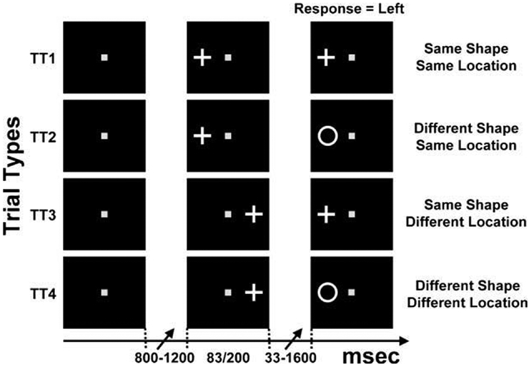
Experimental paradigm. There were four types of trials (TT1–TT4) intermixed randomly in a single run. In this example, trials for a single cue shape (cross) and a single target location (left) are illustrated. The horizontal arrow at the bottom represents time. After fixation (left column; random duration between 800 and 1200 ms), a cue is flashed (83 or 200 ms) either to the left or right of the fixation point (middle column). After a random delay (33–1600 ms), a target is presented which remains on the screen until the observer responds. The observer’s correct response in any of these trials is ‘left’.

2. Methods

2.1. Behavioral methods

We conducted two experiments that were identical in nearly all aspects and hence are combined in the sections below. The only difference between the two experiments was the duration of the cue and the selection of CTOAs. Namely, in Experiment 1 (long cue duration experiment), the duration of the cue was 200 ms and the CTOAs used were 300, 350, 400, 600, 1000, 1800 ms, whereas in Experiment 2 (short cue duration experiment), the duration of the cue was 83 ms and the CTOAs were 116, 350 and 600 ms. The cue duration in Experiment 2 was reduced from that in Experiment 1 to allow for the presentation of the target at a shorter CTOA of 116 ms. The other two CTOAs (350 and 600 ms) in Experiment 2 were chosen to allow for a direct comparison of cueing effects in the two experiments and determine the role of cue duration in our experiments.

2.1.1. Observers

Six observers (two authors and four naïve) participated in the long cue duration experiment and four observers (one author and three naïve) in the short cue duration experiment. Informed consent was obtained from each observer and the study was approved by the Committee for the Protection of Human Subjects at our institution in accordance with the Declaration of Helsinki. We have used a design in which a large quantity of data is obtained from each observer. This is similar to strategies used in previous studies with both humans and monkeys (e.g., Deaner & Platt, 2003; Fecteau & Munoz, 2005). We chose this design in order to facilitate comparisons with animal studies where the use of a large number of observers is impractical.

2.1.2. Apparatus

Observers viewed a Macintosh G5 computer monitor (15 in. LCD, 4 ms off-time, 1280 × 1024, 60 Hz) from a distance of 62.5 cm using a chin-rest. Each pixel was 1.4 arc-min. Experiments were conducted in a dark room. The response to a target was obtained using a custom built box that contained two laterally displaced push button switches (response box). The temporal resolution of response time (RT) data was 100 μs. The software was written in Matlab and utilized the Psych toolbox (Brainard, 1997) for visual stimulus presentation.

2.1.3. Stimulus

A small white square (8 × 8 pixels, 0.2 × 0.2°, 187 cd/sq m) was used as a fixation stimulus and was presented in the center of the dark screen. There were two shapes: a cross and a circular annulus that were used as cues and targets in each experiment (see Fig. 1). The cue and target stimuli had luminance of 187 cd/sq m. Each shape stimulus was constructed in a square of 64 × 64 pixels (1.5 × 1.5°). To keep the total energy nearly constant, the total number of white pixels in cross and circular annulus shapes were 1792 and 2030 pixels respectively.

2.1.4. Procedure

For each observer, choice response time data were collected in five sessions (two observers only completed four sessions), each on a separate day. There were five runs in one continuous session, which were completed in one sitting. After the observer fixated on a cross at the center of the screen, he/she initiated a trial by pressing and holding the two response switches simultaneously. In each trial of a run, after an initial variable fixation period (800–1200 ms), a cue was displayed (see Fig. 1). After the offset of the cue, a variable delay ensued before the presentation of a target. The cue and target were randomly offset horizontally on either side of fixation (5°, eccentricity). They could appear in either the same or different side/location. The shapes of the cue and target were also randomly chosen to be the same or different. Observers were instructed to fixate centrally, to ignore the first cue stimulus, and to respond as quickly as possible to indicate the location of the second target stimulus by releasing the corresponding switch (left or right). Left (right) hand was used to manipulate the left (right) switch. The target remained on the screen until the observer responded. RT were computed by digitizing the analog signals from the switches. To minimize the influence of voluntary attention, before the experiments the subjects were explicitly told that the shape and the location of the first stimulus had no predictive validity for either the shape or location of the following target. Trials in which response times were less than 150 ms were discarded and repeated again. The inter-trial interval was 500 ms. There were 96 trials in each run for the long cue duration experiment (2 locations [−5° and 5°] × 2 cue shapes [circular annulus and cross] × 2 target shapes [circular annulus and cross] × 2 trial types [same vs. different locations for cue and target] × 6 CTOAs). In the short cue duration experiment, there were 48 trials in each run (2 locations [−5° and 5°] × 2 cue shapes [circular annulus and cross] × 2 target shapes [circular annulus and cross] × 2 trial types [same vs. different locations for cue and target] × 3 CTOAs).

2.1.5. Data analysis

2.1.5.1. Cueing effect analyses.

The response time data were sorted into four trial types (TT1–TT4) based on the shape and location of the target relative to those of the cue: (a) same-shape, same location (TT1), (b) different shape, same location (TT2), (c) same-shape, different location (TT3), and (d) different shape, different location (TT4) (see Fig. 1 and Table 1). For each trial type in the long cue duration experiment, there were 6 CTOAs. For each trial type in the short cue duration experiment, there were 3 CTOAs. Trials with erroneous responses (i.e. responses indicating the wrong target location) were eliminated from further analysis of RT cueing effects. These trials were used to evaluate the contribution of any speed-accuracy tradeoffs in our experiments. As described in Table 1, four types of cueing effects (CEs) were computed from the response time data from the trial types (defined above and illustrated in Fig. 1).

Table 1.

Definitions of four cueing effects.

Cueing effect type	Equation
Same-shape spatial cueing (CE1)	TT3–TT1
Different-shape spatial cueing (CE2)	TT4–TT2
Same-location shape cueing (CE3)	TT2–TT1
Different-location shape cueing (CE4)	TT4–TT3

We used non-parametric as well as parametric techniques to analyze the cueing effects in short and long duration experiments. The methodological details of both the analyses are presented in the appendix. The non-parametric technique was used because in many cases the RT data from individual observers and individual CTOAs were not distributed normally (tested using Lilliefors test). Tables A1 (long duration experiment) and A2 (short duration experiment) in the appendix summarize the results of Lilliefors test on RT as well as promptness (1/RT) data obtained from each observer. The number in each cell of the table represents the number of trial types out of four types (as shown in Fig. 1) for which the Lilliefors test rejected the null hypothesis that the data were normal for a given subject and a given CTOA. Zero in a cell in the table means that data for all the four trial types for a given subject and a given CTOA were normally distributed. Note that transforming the RT data into promptness (1/RT) does not eliminate the problem of non-normality in the response time data. We used the parametric technique to confirm the qualitative aspects of the results from the non-parametric analyses.

2.1.5.2. Speed-accuracy tradeoff analyses.

Although error rates were extremely low in these experiments (492 out of 18,240 trials = 2.7% – errors totaled across all subjects and both experiments), speed-accuracy tradeoffs are possible in choice response time experiments (Pachella & Pew, 1968; Swensson, 1972). To examine the role of speed-accuracy tradeoff in our experiments, for each type of cueing effect, we performed a correlation analysis to test if the change in response time (i.e. cueing effect) and change in error were significantly negatively correlated. Each data pair for the analysis consisted of a difference between median RTs and difference between errors in two types of trials (e.g., for CE1, TT1 and TT3) from a single CTOA and a single observer. Data from long and short cue duration experiments were analyzed separately. Thus for each type of cueing effect, there were 36 (6 CTOAs × 6 subjects) and 12 (3 CTOAs × 4 subjects) data points for the correlation analysis of long and short cue duration experiment respectively. Pearson correlation coefficient and its significance value were determined in SPSS for each type of cueing effect and experiment.

2.1.5.3. Practice effect analyses.

We examined whether practice induced adaptive changes previously observed in response times (Ding, Song, Fan, Qu, & Chen, 2003; Pratt & McAuliffe, 1999; Weaver, Lupianez, & Watson, 1998) also occurred in the long cue duration experiment. Practice effects were only examined for the long cue duration experiment because the short cue duration experiment was performed after the long cue duration experiment.

To examine the effect of running repeated sessions on the response times (practice effect), the response time data in the four trial types shown in Fig. 1 were examined as a function of the session number for all CTOAs. Practice effects were also examined for the cueing effects as a function of the session number for all CTOAs. A linear regression analysis was performed for each type of cueing effect to test if the slope of the relationship between the cueing effect and session number was significantly different from zero. In each regression analysis, for each session number, the data were pooled across all the CTDs. The regression analysis was performed using Statview (Abacus, Berkeley, CA). Regression analyses were not performed for the response time data because the effect of practice on response times was substantial and easily seen in the reported statistics.

2.1.6. Modeling methods

We developed a simple model using model neurons with shunting dynamics (Grossberg, 1972). We set the parameters to mimic the repetition suppression property of individual neurons in area LIP and included the property of mutual inhibition among these neurons (see Fig. 2). The neural model of reflexive spatial attention is shown in Fig. 2.

Fig. 2.

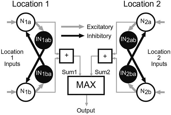
Neural network model of reflexive spatial attention. The pattern of network connectivity is illustrated for two spatial locations (Location 1, Location 2). Shape selective neurons (N_1a, N_1b) and (N_2a, N_2b) encode spatial Locations 1 and 2 respectively. Neurons encoding a given location with different shape selectivity mutually inhibit each other (e.g., N_1a inhibits N^1b and N_1b inhibits N_1a) via inter-neurons (IN_1ab and IN_1ba, respectively). The dynamic firing rate activity from all shape selective neurons encoding a location are summed (Sum1 and Sum2). The output of the model is equal to the larger sum and its target related responses represent the modulatory component of the behavioral response to the target.

There were two spatial Locations, 1 and 2. Each of these spatial locations was encoded by a pool of shape selective neurons. For simplicity, we used two shape selective neurons per location that were selective for shape “a” or “b” (N_1a and N_1b for Location 1, and N_2a and N_2b for Location 2). In order to qualitatively mimic the firing profile of a shape selective neuron in area LIP (Lehky & Sereno, 2007), each shape selective model neuron included a key property of adaptive gain control. The adaptive gain control reduced the effectiveness of a stimulus when presented repeatedly by reducing the output of the model neuron, a property referred to as repetition suppression. We do not know if the repetition suppression property observed in LIP neurons is due to biophysical properties of LIP neurons (as we have implemented with our adaptive gain component) or due to a suppressed input to the LIP neuron. Therefore we do not claim that the implementation we have chosen to functionally mimic repetition suppression is exactly how it is implemented in the brain. We have however chosen to utilize a biophysical mechanism for repetition suppression that has been previously used to implement response adaptation in retinal computations (Abbott, Varela, Sen, & Nelson, 1997; Grossberg, 1972; Ogmen, 1993).

For a given spatial location, each shape selective neuron mutually inhibited the other local shape selective neuron via an inter-neuron (IN_1ab and IN_1ba for Location 1, and IN_2ab and IN_2ba for Location 2). There is indirect evidence of local inhibitory interactions among texture selective neurons in inferotemporal cortex of monkeys (Wang, Fujita, & Murayama, 2003). Wang et al. showed that blocking GABAergic inhibition in inferotemporal cortex caused previously unresponsive cells to respond to textured stimuli. In other words, removal of inhibition broadened the texture selectivity of the investigated cells. To mimic slightly overlapping shape selectivity of the two shape selective neurons, we have arbitrarily introduced a 10% cross-talk at the input of the model. The results of our simulations do not change with or without the 10% cross-talk, though beyond a cross-talk of approximately 40%, the shape cueing effect is largely eliminated. The net activity for each spatial location was obtained by simply summing the activities of all the shape selective neurons. The output of the model was computed by determining the larger of the net activities corresponding to the two spatial locations. The dynamic mechanism performing a combination of such spatially localized signals was not explicitly implemented in our model but could be implemented by a winner-take-all type network. The model was simulated using Matlab (The MathWorks, Natick, MA). The differential equations governing the dynamics of all the neurons in the model and the parameters of the model (see Table A3) are described in the appendix.

3. Behavioral results

Four types of cueing effects (see Table 1) were computed from the choice response times obtained in the long and short cue duration experiments using non-parametric and parametric analyses and are tabulated in Tables A4a-e in the appendix. A positive (negative) value for a cueing effect represents facilitation (inhibition). Significant cueing effects are denoted by a bold font in Tables A4a-e. The cueing effects from non-parametric and parametric analyses are qualitatively very similar with only small quantitative differences (see Tables A4a-e in the appendix). In general cueing effects were significant for fewer CTDs with parametric analyses (18 vs. 21), but the fewer statistical significances do not alter any of our findings or conclusions. Thus, for sake of statistical appropriateness and clarity, we will only discuss the results of the non-parametric analyses in greater detail. The quantitative differences between non-parametric and parametric analyses occur because in most cases the RT distributions are not normal and the parametric analyses assumes them to be normal, which results in higher variances compared to those in non-parametric analyses.

3.1. Spatial cueing effect

The spatial cueing effects (CE1 and CE2 in Table 1) determined by non-parametric analyses from long (solid lines) and short (dashed lines) cue duration experiments are shown in Fig. 3 (top row). The data from trials in which the cue and target had the same shape (CE1) are shown in Fig. 3a. The data from trials in which the cue and target had different shapes (CE2) are shown in Fig. 3b.

Fig. 3.

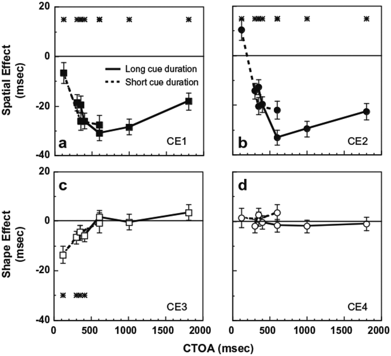
Cueing effects as a function of CTOA. The four types of cueing effects shown are: (a) Same-shape spatial cueing effect (top, left panel; CE1). (b) Different-shape spatial cueing effect (top, right panel; CE2). (c) Same-location shape effect (bottom, left panel; CE3). (d) Different-location shape effect (CE4; bottom, right panel). The asterisk in each plot indicates that at that particular CTOA the corresponding cueing effect is significant. The error bars represent ± 1 SE of median. The solid (dashed) lines correspond to data from the long (short) duration cue experiment.

In the long cue duration experiment, there was a significant inhibitory spatial cueing effect at all CTOAs tested (range: 300–1800 ms) regardless of whether the cue and target had the same or different shapes (asterisks for long cue duration in Fig. 3a and b, also see Tables A4a and b, long cue duration). The inhibitory spatial cueing effect averaged across all CTOAs was 23.5 ms for same shape condition and 22 ms for different shape condition. The inhibitory spatial cueing effects for CTOAs up to 400 ms were larger when the cue and target shapes were the same compared to different (mean difference = 5.7 ms; see Table A4e for comparisons). The inhibitory spatial cueing effect increased as CTOA increased from 300 to 600 ms regardless of whether the cue and target had the same or different shapes. The slope of increase was higher when the shape of the cue and target were the same (62.5 ms/s CTOA) compared to different (40.5 ms/s CTOA). Beyond a CTOA of 600 ms, the inhibitory spatial cueing effect decreased and the rate of decrease was similar in the same and different shape conditions (approximately 38 ms/s CTOA).

The short cue duration experiment extended CTOAs to shorter values (range: 116–600 ms). For the shortest CTOA in this experiment, which was 116 ms, the sign of the spatial cueing effect depended on whether the cue and target had the same or different shapes. When the cue and target had different shapes, a significant facilitatory spatial cueing effect of 10.4 ms was observed, while for the same CTOA, when the cue and target had the same shape, a significant inhibitory spatial cueing effect (6.5 ms) was observed. At this shortest CTOA, the facilitatory spatial cueing effect was reduced significantly when the cue and the target had the same shape compared to different (p < 0.001; for other CTOAs see Table A4e).

3.2. Shape effect

The shape cueing effects (CE3 and CE4 in Table 1) determined by non-parametric analyses from long (solid lines) and short (dashed lines) cue duration experiments are shown in Fig. 3 (bottom row). The data from trials in which the cue and target were presented at the same location (CE3) are shown in Fig. 3c. The data from trials in which the cue and target were presented at different locations (CE4) are shown in Fig. 3d.

In the long cue duration experiment at the shorter CTOAs, there was a significant slowing of response for the same shapes on cued trials, when cue and target were presented at the same location (CE3; asterisks at 300 and 400 CTOA in Fig. 3c, solid line; also see Table A4c). This inhibitory shape effect (CE3) in cued trials was maximal (6.5 ms) at the shortest CTOA of 300 ms and then decreased to virtually zero (slight, 1.6 ms, nonsignificant facilitatory effect) as CTOA increased to 600 ms. The slope of decrease of the inhibitory shape effect was 27.1 ms/s CTOA. On the other hand, in uncued trials, when the cue and target were presented at different locations, the response times did not depend on whether the cue and target had the same or different shape at any CTOA (CE4; no asterisks in Fig. 3d, solid line; also see Table A4d).

In the short cue duration experiment, there was also a significant slowing of response on cued trials when the cue and target had the same compared to different shapes (asterisks in Fig. 3c, dashed line; see Table A4c). The inhibitory shape effect in cued trials was maximal (13.6 ms) at the shortest CTOA of 116 ms and then decreased to virtually zero (0.7 ms) as CTOA increased to 600 ms. The slope of decrease of the inhibitory shape effect was 26.7 ms/s CTOA and was similar to that in the long cue duration experiment, suggesting that the duration of the cue does not alter the shape effect (see also Fig. 4) in our experiments. Further, as in the long cue duration experiment, no shape effect was found at any CTOA in uncued trials (no asterisks in Fig. 3d, dashed line; see Table A4d, short cue duration).

Fig. 4.

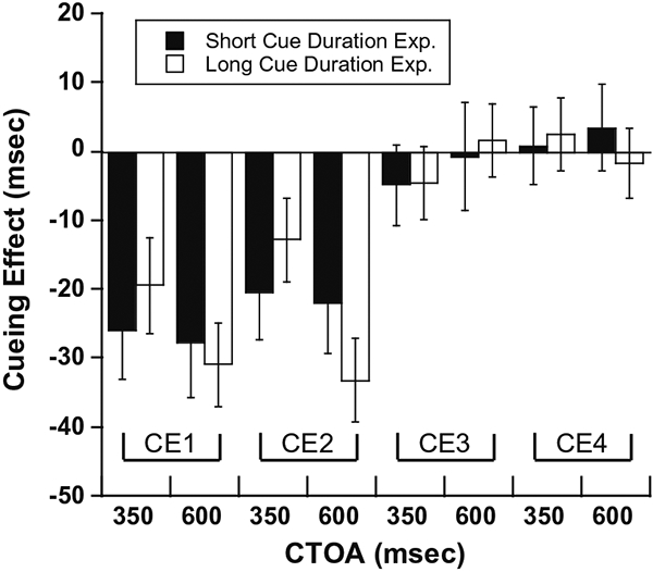
Comparison of cueing effects in the short and long cue duration experiments. The four types of cueing effects (CE1–CE4) are shown separately for short (black bars) and long (clear bars) cue duration experiments. For each experiment and each type of cueing effect, cueing effects are shown for CTOAs of 350 and 600 ms. The error bars represent 95% confidence interval of the median.

3.3. Relationship between changes in response times and response errors

Do the response time changes in our experiments correlate with corresponding changes in response errors in a manner that can be fully explained by a speed-accuracy tradeoff? First, the response error changes in our experiments were very small (mean error change across cueing effects (CE1–CE4), CTOAs and subjects: 0.08 ± 0.04% SD and 0.05 ± 0.03% SD for long and short duration experiments respectively). There was no evidence of a significant relationship between the response time change and the percentage change in response error for any of the four types of cueing effects and for both the experiments. The best correlation consistent with speed-accuracy tradeoff was obtained for CE3 (r = −0.26, p = 0.13) in the long cue duration experiment. Thus, a speed-accuracy tradeoff did not play a significant role in our experiments.

3.4. Effect of practice on response times and cueing effects in long duration experiment

For all types of trials (TT1–TT4), and for all CTOAs, the average response time decreased as session number increased, indicative of a practice effect occurring in behavioral responses in the first sessions of the long duration experiment. The response times averaged across all trial types and all CTOAs were 315.4 ± 14.9 SD, 288.6 ± 14.2, 277.7 ± 13.9, 276.7 ± 15 and 278.7 ± 9.7 ms for sessions 1–5 respectively. The decrease in response time was highest in the initial sessions and reached a lower asymptote after the third session.

Further, there was no evidence of a relationship between session numbers and cueing effect for any type of cueing effect (CE1: p = 0.1; CE2: p = 0.2; CE3: p = 0.7; CE4: p = 1.0). Out of the four regression models, the model for same-shape spatial cueing explained the most variance and its R² was still only 0.091. These results are consistent with results from previous studies by Pratt and Mcauliffe (1999) and Collie et al. (2000) showing that practice effects do not interact with cueing effects. The practice effect observed in response times and a lack of change in cueing effect as a function of session number suggest that practice-induced-changes occurred in a similar fashion for all types of trials.

3.5. Comparison of cueing effects in short and long cue duration experiments

For the two CTOAs where the short cue experiment and long cue experiment overlapped (350 and 600 ms), in Fig. 4, we replotted the cueing effects from Fig. 3 along with the 95% confidence intervals. For each cueing effect (CE1–CE4), and for each CTOA (350 and 600), the 95% confidence intervals in the short and long cue duration experiments show an overlap. This simple test suggests that in our experiments, the duration of the cue does not substantially alter the different cueing effects.

4. Modeling results

To examine the basic mechanics of the model, we first applied a pulse stimulus of 50 ms to the neuron selective for shape ‘a’ at spatial Location 1. All other inputs were held at zero. All the neurons in the model have continuous valued outputs representing their firing rates. The shape selective neuron N_1a responded by increasing its firing rate quickly from the baseline level and then gradually decreasing its firing rate to an elevated baseline level (Fig. 5a, top row). The inter-neuron that N_1a projects to is IN_1ab and it responds to the firing of N_1a by increasing its output from the baseline and then decreasing it relatively slowly towards an elevated baseline. The elevated baseline firing rate is also indirectly visible in the elevated output of the inter-neuron IN_1ab (Fig. 5a, bottom row) which receives its input from N_1a. This dynamic firing rate profile was in good qualitative agreement with extracellular recordings in areas LIP and AIT in monkeys (Lehky & Sereno, 2007). Note that there is no special cellular mechanism in N_1a to cause the elevation of baseline firing rate after stimulation, it is instead a phenomenon resulting from equilibrium in the network dynamics. In addition, elevated baseline firing rate after stimulation in area LIP in monkeys has been previously demonstrated (see Fig. 3 in Lehky & Sereno, 2007). Further, the adaptive gain component within N_1a quickly reduced the gain in the excitatory synapse after the onset of the stimulus and then gradually returned it to the pre-stimulation level (Fig. 5a, middle row). This adaptive gain component mimics the neural mechanism of repetition suppression in the model.

Fig. 5.

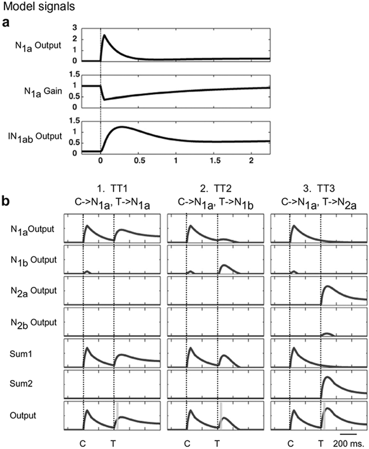
Simulated neuronal activity traces in response to a single pulse input simulating the presentation of shape “a” in location 1. (a) A 50 ms pulse is applied to N_1a at time 0 (dotted vertical lines). The inputs to the other three neurons were set to zero. The top panel shows the firing rate output of N_1a. Other shape selective neurons in the model have similar dynamic properties. It shows a rapid increase in firing rate followed by a slow decay to an elevated baseline. The middle panel shows the gain change that occurs within N_1a for the excitatory input of N_1a. The lower panel shows the firing rate changes in the inter-neuron IN_1ab. (b) Responses of model neurons for a cue and a target presentation. Each column of traces represents one of three types of cueing protocol: column 1, TT1 – cue (C) and target (T) have same shapes and are presented at the same location (left column), column 2, TT2 – cue and target have different shapes but are presented at the same location (middle column), and column 3, TT3 – cue and target have same shapes but are presented at different locations (right column). The cue duration is 50 ms and CTOA is 400 ms. The target stays on until the end of simulation. The left (right) vertical dotted line in each column represents the onset of cue (target). The first four rows show the firing rates of N_1a, N_1b, N_2a and N_2b respectively. The following two rows show the summed activity for each encoded location (Sum1, Sum2). The output of the model is shown in the bottom row. The vertical gray bar in each column of the bottom row indicates the temporal window over which the model’s output is integrated for computations of the cueing effects presented in the following two figures.

Next, to examine the mechanics of the model during a standard spatial cueing paradigm (Posner & Cohen, 1984), we used a 50 ms pulse signal followed by a step signal in various spatio-temporal input configurations. The pulse and step input signals represented the cue and the target respectively. The reason a step stimulus is used for target is that in many behavioral paradigms (including ours), the target is left on the screen until the observer responds. Fig. 5b illustrates simulated neuronal activity traces when the delay between the onset of the pulse signal and the onset of the step signal (or CTOA) was 400 ms. We simulated two types of spatially cued trials: (1) cue and target had the same shape (TT1; same-shape cued trial); and (2) cue and target had different shapes (TT2; different-shape cued trial). Additionally, we also simulated a spatially uncued trial in which cue and target had the same shapes (TT3). Note that for the current modeling purposes, the relative shapes of cue and target in spatially uncued trials are irrelevant and do not change the model’s output (i.e. TT3 or TT4; this is in agreement with the behavioral data, see Fig. 3d) because in these conditions the cue and the target would excite neurons corresponding to different spatial locations and presently there are no long-distance shape interactions in our model between the two spatial locations. For each of the three tested conditions (TT1–TT3), the firing rate profiles of all the shape selective neurons in the model, the net activity corresponding to each spatial location, and the model output are illustrated in Fig. 5b.

In the same-shape cued trial (TT1), the cue and target pulses stimulated the same neuron (N_1a). The cue therefore had a suppressive effect on the response of the subsequent target due to the adaptive gain change it induced within N_1a (Fig. 5b, column 1, N_1a output for T). On the other hand, in the different-shape cued trial (TT2), the cue stimulated N_1a and the target stimulated N_1b. In this case, the cue still had a suppressive effect on the response of the target, but it was due to the inhibitory effect of IN_1a on N_1b (Fig. 5b, column 2, N_1b output for T). In the uncued trial (TT3 shown), the cue and target stimulated neurons N_1a and N_2a respectively, and because they encoded different spatial locations, the response of N_2a neurons was unaffected by the cue driven adaptive gain change within N_1a or mutual inhibition in the network (Fig. 5b, column 3, N_2a output for T). Note that the target related output of the model in the uncued trial was greater in magnitude than target related response in both cued trials. In other words, regardless of the shapes of the cue and the target, the cueing effect was inhibitory (examples of IOR). In order to examine the effect of CTOA on the cueing effect, the output activity corresponding to the target presentation at each spatial location was integrated for 25 ms. The integration window started at 25 ms after the onset of the target (gray vertical bar in Fig. 5b, bottom rows). An integration window of 50 ms duration was also tested and was found to yield qualitatively similar simulation results to those found with a 25 ms integration window.

To quantify the typical spatial cueing effect (i.e. CE2), the integrated output of the model as a function of CTOA was determined for the different-shape cued (TT2; i.e. similar to Posner and Cohen’s reflexive paradigm (1984) in which the cue was a rectangular frame and target was a filled square) and uncued trials (TT4). We made two basic assumptions: (1) the output of the model represents a modulatory effect on the observer’s response to the target (this point is revisited in the discussion section); and (2) only sustained signals from the visual on-pathway are considered as inputs to the model. The duration of the cue was 50 ms and the CTOA varied from 75 to 1800 ms. The target remained on until the end of simulation. The spatial cueing effect was computed as the difference between the integrated output in the cued and the uncued trials. In agreement with existing empirical data (e.g., Posner & Cohen, 1984), the simulated spatial cueing effect shown in Fig. 6 was facilitatory for short CTOAs and inhibitory for long CTOAs (inhibition of return or IOR). In addition, the inhibitory spatial cueing effect lasted substantially longer than the facilitatory spatial cueing effect. Note that the parameters of the model (Table A3 in the appendix) were adjusted only to capture the qualitative nature of the behavioral data from Posner’s type cueing paradigm.

Fig. 6.

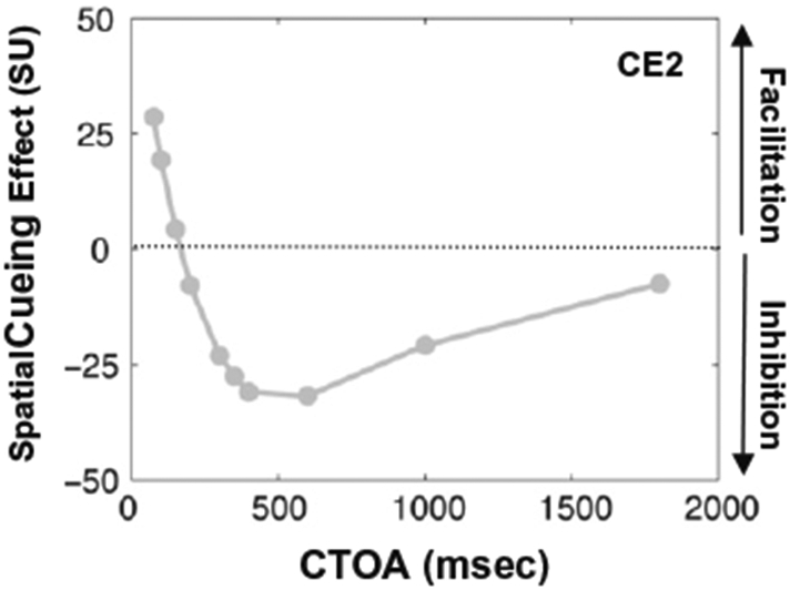
Simulated cueing effect as a function of CTOA for a typical reflexive spatial attention paradigm in which cue and target have different shapes. Note that the unit for the y-axis is simulation unit (SU) and is also used in Fig. 7. To convert the integrated activity of model’s output to SU, it was divided by 0.001. The conversion to SU was performed to keep the plotted data in a reasonable range. A facilitatory cueing effect occurs for short CTOAs while an inhibitory cueing effect (IOR) occurs for long CTOAs. The duration of the cue is 50 ms and CTOAs range from 75 to 1800 ms. The target remains on until the end of simulation.

One may ask why is that using a model with so many free parameters we only modeled the qualitative aspects of the behavioral data? It is important to note that we start with a standard model for the neuron. This model of the neuron is commonly used in neural network models to study visual perception (Grossberg, 1972; Ogmen, 1993) and parallel distributed processing (Rumelhart & McClelland, 1986). Because the model of the neuron aims to capture the biophysical properties of a biological neuron, it has many parameters. We set these parameters to qualitatively mimic the physiology of neurons found in monkey area LIP. We utilize these neurons in a small network to explain behaviorally measured reflexive cueing effects. Our purpose with the modeling is not to determine all the cellular level parameters for such a network, nor to try to exactly mimic the physiology or behavior. Our purpose with the modeling is to gain significant insights, at a simple scale, about the role of processes such as adaptive gain control and mutual inhibition and to obtain qualitative characterizations that are more or less invariant with respect to specific parameter choices.

Finally, we examined the simulated responses in all four types of cueing conditions (CE1–CE4) that were used in our behavioral experiments. For example, the shape effect (CE3) was examined by simulating the different-shape cued trials (TT2) and comparing the simulations to those of the same-shape cued trials (TT1). To facilitate a direct comparison to the data shown in Fig. 3, the cue duration for these simulations was 200 ms for CTOAs from 300 to 1800 ms and 83 ms for CTOA of 100 ms. The predicted outcomes of the model are in qualitative agreement with our experimental data. The facilitatory spatial cueing effect at shorter CTOAs was reduced substantially when the shapes of the cue and the target were the same compared (CE1) to when they were different (CE2; see Fig. 7, column 1, top (7a) vs. middle (7b) row, compare to behavioral data in Fig. 3a vs. 3b). The difference between the same-shape cued and different-shape cued trials (CE3) yielded the shape effect, which illustrates the suppressive effect of using the same shape for the cue and the target at short CTOAs (Fig. 7, column 1, bottom row (7c), compare to behavioral data in Fig. 3c).

Fig. 7.

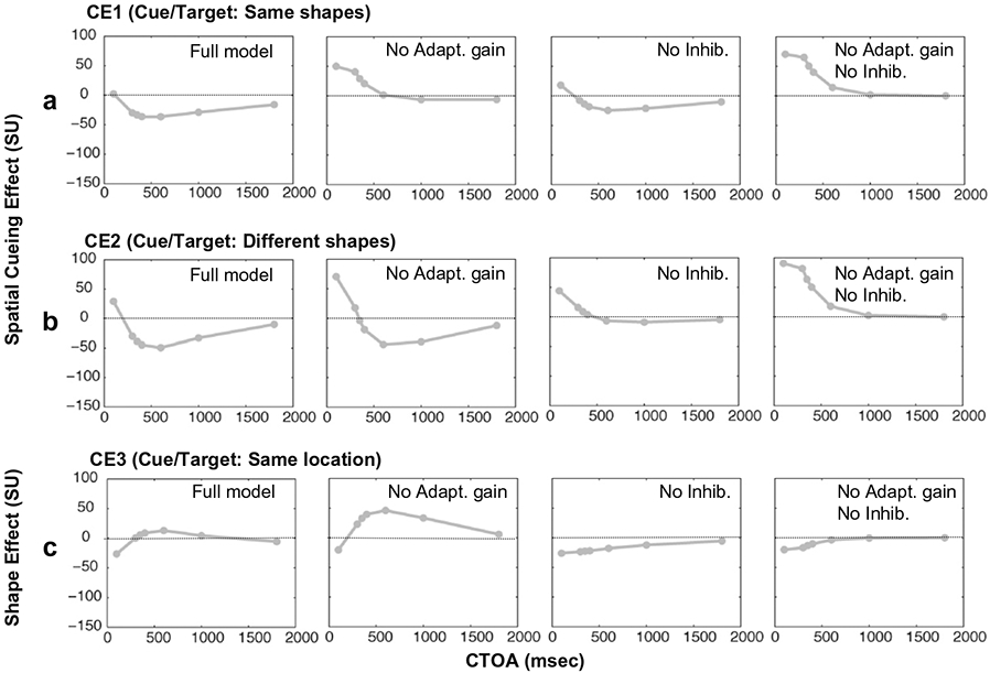
Simulated cueing effects as a function of CTOA in normal and lesioned models. Lesioned models explore the effects of adaptive gain control and mutual inhibition on these cueing effects. The unit for the y-axis is SU as defined in Fig. 6. The top and middle rows represent two spatial cueing conditions: Top row – cue and target have same shapes (CE1). And middle row – cue and target have different shapes (CE2). The bottom row shows the shape cueing effect when cue and target are at the same location (CE3). The different columns show simulations for a model in which: Column 1 – both adaptive gain control and mutual inhibition are enabled. Column 2 – adaptive gain control is disabled. Column 3 – mutual inhibition is disabled. And, column 4 – both adaptive gain control and mutual inhibition are disabled. The duration of the cue is 200 ms for CTOAs ranging from 300 to 1800 ms and 83 ms for a CTOA of 100 ms. These cue durations are used because they match the empirical data in Fig. 3. The target is left on until the end of simulation.

One of the goals of our study is, with the aid of modeling, to determine how known physiological processes of adaptive gain control and mutual inhibition combine and test whether they can explain in a unified manner (1) the general behavior of spatial attention, i.e. facilitation at short CTOAs and inhibition at longer CTOAs, (2) the dependence of spatial attention on shapes of the cue and the target, and (3) the behavior of shape cueing. In order to determine the relative contributions of mutual inhibition and adaptive gain control on the spatial and shape cueing effects, “lesions” of these two mechanisms were simulated in the model. When only the adaptive gain control was removed from the model, the facilitatory spatial cueing effect at short CTOAs was enhanced (Fig. 7, column 1 vs. column 2, top and middle rows). The model no longer showed IOR when the cue and the target had same shapes (Fig. 7, column 2, top row). In addition, the target related neuronal activity remained at a plateau until the end of simulation as opposed to decaying to an elevated baseline as shown in Fig. 5a (top row). When only the mutual inhibition was removed from the model, there was primarily a decrease in IOR at all CTOAs and a small increase of the facilitatory spatial cueing effect at short CTOAs (Fig. 7, column 1 vs. column 3, top and middle rows). In addition, the corresponding inhibitory shape effect now lasted for a couple of seconds instead of just occurring at short CTOAs (Fig. 7, column 3, bottom row). If adaptive gain control and mutual inhibition were both removed from the model, the facilitatory spatial cueing effect was enhanced and IOR was absent regardless of the shapes of the cue and the target (Fig. 7, column 1 vs. column 4, top and middle rows). Notice that the shape effect in this reduced model was compressed compared to that in the full model.

5. Discussion

We have combined behavioral experiments and mathematical modeling to investigate the neural substrates of spatial and shape effects on reflexive spatial attention. We show empirically that the reflexive facilitatory spatial cueing effect is reduced when the shapes of the cue and the target are the same compared to when they are different. Regardless of the shapes of the cue and the target, a robust reflexive inhibitory spatial cueing effect (or IOR) at long CTOAs is also observed. It should be emphasized that the spatial cueing effects obtained using our paradigm are very similar to those obtained in a paradigm in which fewer data are obtained from each observer but a large number of observers are tested (e.g., Posner & Cohen, 1984). This suggests that reflexive spatial cueing effect is a robust effect and its detection does not depend on a particular paradigm or method of analyses. In addition, we have shown that a significant reflexive inhibitory shape effect is observed. This effect decreases as CTOA increases. These spatial cueing effects and their dependence on shape are well explained by a model consisting of a network of shape selective neurons.

5.1. Role of repetition suppression and mutual inhibition in reflexive cueing effects

As demonstrated in Fig. 7 (top row, column 2 vs. column 1), the adaptive gain property within individual neurons in the model determines the presence or absence of IOR at long CTOAs when the cue and the target have same shapes. Because our data shows the presence of IOR at long CTOAs when the cue and target have same shapes, we infer that the repetition suppression effect observed in physiology is critically involved in the generation of behaviorally observed IOR, as first suggested by Lehky & Sereno (2007) and see also Sereno et al. (2010).

The shape effect measured empirically (Fig. 3c) is in good qualitative agreement with the model’s prediction (Fig. 7, bottom row (7c), first column). As seen in Fig. 7 (bottom row, third column vs. first column), mutual inhibition substantially alters the time course of the shape effect. This suggests that cueing effects that involve features may not only depend on spatial interactions but also depend on mutual inhibition among feature selective neurons representing the same spatial location. Given that shape is encoded differently in different cortical areas (Lehky & Sereno, 2007), it may be possible to tease apart whether these shapes effects on reflexive spatial attention are coming from dorsal or ventral stream areas (Red, Patel, & Sereno, 2010).

5.2. Relationship between model output and decreasing RT with increasing CTOAs

A decrease in behavioral response times with increase in CTOA has been reported in our behavioral findings as well as several other studies (Kwak & Egeth, 1992; Maruff et al., 1999; Maylor, 1984; Maylor & Hockey, 1987; Posner & Cohen, 1984; Pratt & McAuliffe, 1999; Tassinari et al., 1994). These behavioral changes are likely dependent in part on the timing and distribution of targets. The output of our model cannot be used directly to generate the decreasing response times with increasing CTOAs. In our short cue duration experiments we found that the median response times in same shape spatially cued trials (TT1, combined from all the sessions) decreased as CTOA was increased from 116 to 350 ms (RT₁₁₆ = 332.9 ± 2.8 SE, RT₃₅₀: 291.5 ± 3.0 ms). In contrast, for the same range of CTOAs, the model’s output decreased as CTOA was increased. This decrease in model’s output would result in an increase in the behavioral response time. One simple solution would be to add our model’s output with a signal that represents the increasing expectation of the target as a function of CTOAs. This signal should be based on documented and observed decreases in behavioral response times with increasing CTOAs. Such a solution would suggest that the decrease in response time with increasing CTOAs is independent of the reflexive attentional effects.

Further, our experimental results indicate a practice effect in early sessions. There was a reduction in average response times as a function of session number in all types of trials. However, in the same trial type, the cueing effect remained largely constant across session (not shown currently, but was shown during the review process). A lack of dependence of facilitatory and inhibitory cueing effects on session number has been previously reported (Collie et al., 2000; Pratt & McAuliffe, 1999). The reduction in response times with session number without corresponding changes in cueing effects are consistent with our assumption that output of the model represents a signal which modulates an ongoing response which is generated by a combination of neural outputs. The reduction in response times with increase in session number can be attributed to changes in other aspects of the neural substrate. However, there is one report that shows a reduction in IOR with practice (Weaver et al., 1998).

5.3. On independence of facilitatory and inhibitory cueing effects

One of the strongest evidence in favor of independent mechanisms is the suggestion that the facilitatory cueing effect occurs only when the cue and target are presented at the same retinal location while an inhibitory cueing effect occurs only when the cue and target are presented at the same environmental or allocentric spatiotopic location (i.e. location in the external physical space; Maylor & Hockey, 1985; Posner & Cohen, 1984). In the covert orienting experiment of Maylor and Hockey (1985), the subject made an eye movement to a second fixation target after the cue and before the target was presented. They found that IOR was substantially larger when the target shared the same location as the cue in the environment (“environmental” coordinates, e.g., the same location on the computer monitor, but a different location on the retina) compared to if the target shared the same retinal location (retinal coordinates, the same location on the retina, but a different location on the computer monitor). Nevertheless, there was still a small amount of IOR observed in the retinal coordinate cueing condition. An alternative explanation for their findings is that retinotopic and environmental IOR are physiologically separable mechanisms. An additional possibility is that the reduction of retinotopic IOR may be due to their experimental protocol. Unlike in the standard IOR paradigm, in Maylor and Hockey’s (1985) experiments, after presentation of the cue, a saccadic eye movement was directed towards a fixation target, which was always present in the visual field. Such a voluntary movement is thought to engage mechanisms of voluntary attention. It is known that voluntary orienting can inhibit reflexive orienting (Seidlits, Reza, Briand, & Sereno, 2003; Sereno, 1992). Thus, perhaps this additional voluntary eye movement reduced the magnitude of retinotopic IOR but did not similarly affect environmental IOR. The exact nature and specificity of these effects and interactions are not known, but in their presence, it is conceivable that the results of the above experiments do not rule out the possibility that covert reflexive spatial facilitation and inhibition could be mediated by a single neural network operating either in a retinal or “environmental” coordinate system.

In other reports, independence of facilitatory and inhibitory mechanisms is inferred by observing corresponding cueing effects in non-standard stimulus conditions. For example, in some studies facilitation at short CTOAs is either not observed or an inhibitory cueing effect is instead observed (Lambert et al., 1991; Tassinari & Berlucchi, 1993; Tassinari et al., 1994). These data are used to refute the claim of a causal relationship between facilitatory and inhibitory cueing effects, i.e. a claim that facilitation at short CTOA causes inhibition at long CTOA (Maylor, 1984). However, the absence of facilitation at a short CTOA should be cautiously interpreted. First it should be noted that delays in the visual system are not constant, they depend on various spatial and temporal attributes of the visual stimuli (e.g., eccentricity, luminance, duration). Thus, if spatial and temporal characteristics of the cue and the target are different, similar cue and target presentation timings could yield different physiological and thus perceptual responses to the target. Second, if the temporal duration of the target is shortened as in the study of Tassinari et al. (1994), its neural processing time could increase due to processing of a less effective stimulus that lengthens the operative CTOA for brain areas higher up in the processing hierarchy. A shortened target duration also makes the target vulnerable to forward masking which is known to directly depend on the ratio of the cue to target energies (Breitmeyer & Ogmen, 2006). In experiments that have shown significant facilitation at short CTOAs (Maylor & Hockey, 1985; Posner & Cohen, 1984), the target was left on the screen until the observer responded, eliminating the problems of forward masking and processing time increase. The simulated facilitatory cueing effect (not shown) for a CTOA of 100 ms (cue duration = 50 ms) did not change whether the target was a 50 ms pulse or lasted until the end of simulation, suggesting that empirical differences in the experiments of Tassinari et al. (1994) and others are likely due to differences in the contribution from other mechanisms important for the strength of the stimulus representation (e.g., forward masking and processing time considerations).

In our model, facilitatory and inhibitory cueing effects occur in a single network of shape selective neurons. In addition, we show that the facilitatory cueing effect can be modulated by the relative shapes of the cue and the target. Thus, we show that the presence of an inhibitory cueing effect and concurrent absence of a facilitatory cueing effect does not necessarily imply that two independent mechanisms underlie the two types of cueing effects.

5.4. Object associated cueing effect

There are numerous demonstrations of ‘reflexive’ facilitatory and inhibitory cueing effects in situations where the cueing is associated with an object (Abrams & Dobkin, 1994; Gibson & Egeth, 1994; McAuliffe, Pratt, & O’Donnell, 2001; Ro & Rafal, 1999; Tipper, Driver, & Weaver, 1991; Tipper, Jordan, & Weaver, 1999; Tipper, Weaver, Jerreat, & Burak, 1994; Tipper et al., 1997) rather than space. But, some of these object-based cueing effects are not robust to stimulus parameter variations (Muller & von Muhlenen, 1996; Ro & Rafal, 1999). Early experiments that produce these object-based cueing effects utilize a moving stimulus of some kind. By moving a set of objects, the idea is to present the cue and target at different spatial locations (i.e. the target always appears in an uncued spatial location) but associate them with the same (cued condition) or different (uncued condition) objects. The cueing effect could however reflect reflexive or voluntary, spatial or feature-based modulations of neuronal activity or some combination of these modulations. Hence, the presence of object-based cueing observed in paradigms involving stimulus motion does not necessarily challenge the neural network model proposed here.

More recently, it is shown that spatial IOR can be modulated by static features surrounding a brief cue (Morgan, Mathew, & Tipper, 2005). They found that spatial IOR is substantially larger when the object surrounding the brief cue was identical to that surrounding the subsequently presented target (identical condition) compared to when the surrounding objects for cue and target were unrelated (unrelated condition). Interestingly, if we compare their results in the identical condition with those in the unrelated condition, then a strong inhibitory “same” object cueing effect is found for spatially cued trials (approximately 31 ms) and a weak inhibitory “same” object cueing effect is found for spatially uncued trials (approximately 7 ms). These results agree qualitatively with the shape cueing effect found for spatially cued and uncued trials in our experiments (Fig. 3c and d). Thus the model presented here may be able to account for the qualitative aspects of the object associated cueing effects if we assume that similar to shape selective neurons, there are also object selective neurons organized in a manner proposed by the model.

5.5. Spatial cueing vs. priming paradigm

There is some resemblance of a priming paradigm with the spatial cueing paradigm. An important difference between the two paradigms however is the task of the observer and thus the neural signals utilized to perform the tasks. Klotz and Wolff (Klotz & Wolff, 1995) used a choice response time priming paradigm in which they varied the relative shapes of the prime and the target. They also used a control condition in which the target was presented without a preceding prime. Observers were asked to choose the appropriate response as quickly as possible based on the shape of the target (e.g., key A if the target shape was A and key B if the target shape was B). Note that in our spatial cueing paradigm, the observer is instead asked to indicate the location of the target. Klotz and Wolff found that response times were shorter in trials in which the shapes of prime and target were congruent compared to those in the control condition. Of relevance here, they also found that the response times were longer in trials in which the shapes of prime and target were incongruent compared to those in the control condition indicating an inhibitory interaction between the mechanisms responsible for processing the shapes of prime and target. In our model, if we separately examine the responses of the two shape selective neurons encoding a single location, the target related response would be consistent with the behavioral outcome in Klotz and Wolff’s priming experiment. Note that for explaining results of our spatial cueing experiments, we sum the responses from the two shape selective neurons encoding a single location.

5.6. Models of attention

Over the years, many models of covert visual orienting have been proposed (Shipp, 2004). Almost without exception, attentional models include a single salience map, a spatial map which encodes the location of the most salient activation pattern which points to other maps which encode the features of various objects (e.g., color map). In computer analogy, the salience map is a 2-D array that holds the index value which points to another set of maps. The index represents the location of the attended object.

The exact neural locus of a unitary “salience map” as hypothesized by many models is unknown. One study suggests that neurons in LIP may represent visual salience (Gottlieb, Kusunoki, & Goldberg, 1998). In a review on the potential neurophysiological implementation of the “salience map”, Fecteau and Munoz (Fecteau & Munoz, 2006) suggest that the salience map may be implemented implicitly in the oculomotor network. The necessity for a unitary “salience map” in guiding attention has also been challenged (Desimone & Duncan, 1995). Our data and model suggests that reflexive spatial attention effects may result from any brain area showing repetition suppression and mutual inhibition. Thus, in contrast to the idea of a unitary or small network of areas that result in a “salience map”, we suggest reflexive spatial attention may be a distributed property of many areas. Further, for this reason, there may be many forms of reflexive spatial attention, depending on the properties represented in these local networks.

Finally, many of these models utilize an explicit mechanism to explain the phenomenon of inhibition of return observed in reflexive visual attention paradigms (Heinke & Humphreys, 2003; Itti & Koch, 2000; Koch & Ullman, 1985; Shipp, 2004). In our model, IOR results implicitly from repetition suppression and mutual inhibition within the neuronal network. One model in which IOR may occur implicitly within the neuronal network is the model by Deco et al. (Deco, Pollatos, & Zihl, 2002), though this model has mainly been applied to voluntary attention.

6. Summary

In summary, we show that spatial cueing effects depend on the shapes of the cue and the target. In addition, we develop a simple physiologically plausible neural network model. This model is built using adaptive gain control and mutual inhibition, neuronal and network properties that are widespread in areas in the dorsal and ventral visual cortical streams. The model shows that using the above two properties, reflexive attentional effects including both facilitation at early time intervals and inhibition at later time intervals can be explained in a unified manner. This finding suggests one need not postulate separate independent mechanisms for reflexive attentional facilitation and IOR. Further, the model can account for the effect of shapes on spatial cueing reported here. In contrast to previous models of reflexive spatial attention that require centralized computation of salience (see e.g., Shipp, 2004), our model is suggestive of a distributed architecture of reflexive attention in which salience may be computed in parallel in multiple maps across the brain.

Appendix A

A.1. Non-parametric analysis of within observer cueing effects using rank-sum method

We describe below the method used for computing and analyzing cueing effects by using, as example, the same-shape spatial cueing effect (CE1) at a single CTOA in the long cue duration experiment. All other cueing effects were computed similarly by choosing the data sets from appropriate types of trials. We describe the whole procedure as a series of steps.

Table A1.

Summary of Liliefors test results for long cue duration experiment.

Subject	CTOA (ms)
	300	350	400	600	1000	1800
RT data
S1	0	0	0	0	0	1
S2	1	0	3	1	1	3
S4	2	2	1	0	0	0
S5	0	1	1	0	1	1
S6	0	0	0	1	3	2
S7	2	1	1	1	1	0
(1/RT) data
S1	0	1	0	0	2	3
S2	1	0	1	0	0	1
S4	1	3	1	0	0	0
S5	1	0	1	1	0	0
S6	2	1	0	1	2	0
S7	2	1	0	0	0	0

Table A2.

Summary of Lilliefors test results for short cue duration experiment.

Subject	CTOA (ms)
	116	300	350
RT data
S3	1	0	0
S4	0	0	0
S5	1	1	1
S7	0	0	1
(1/RT) data
S3	1	0	1
S4	1	0	1
S5	1	1	2
S7	1	0	1

Table A3.

Values of various parameters in the tested model.

Description	Label	Value
Passive decay constant of shape selective cell (SSC)	Ax	5
Upper bound of excitatory membrane activity for SSC	Bx	1
Lower bound of inhibitory membrane activity for SSC	Dx	−1
Excitatory synaptic gain for SSC	ωx,exc	1
Inhibitory synaptic gain for SSC	ωx,inh	1
Firing membrane activity threshold for SSC	θ	0
Membrane potential to firing rate transformation constant for SSC	σx	10
Excitatory cross-talk between SSCs due to overlapping selectivity	δ	0.1
Rate of gain increase in the synapse of SSC	α	0.9
Maximum gain level in the synapse of SSC	β	1
Relative time scale of the gain modulation dynamics in SSC	τ	1
Baseline input adding a tonic gain level in SSC	J	0
Rate of gain decrease in the synapse of SSC	γ	0.1
Scale factor for excitatory synaptic input in SSC	ηexc	20
Scale factor for inhibitory synaptic input in SSC	ηinh	1
Minimum baseline (or tonic) excitatory synaptic input in SSC	R	0.15
Passive decay constant of inhibitory inter-neuron (IIN)	Ay	2
Upper bound of excitatory membrane activity for IIN	By	1
Excitatory synaptic gain for IIN	ωy,exc	1
Membrane potential to firing rate transformation constant for IIN	σy	5
On state level of external excitatory input signal to SSC	Iexc: on	10
Off state level of external excitatory input signal to SSC	Iexc: off	0

1. For each observer i, pool RTs in same-shape same-location trials (TT1) from different sessions and store them in a vector X_i and pool RTs in same-shape different-location trials (TT3) and store them in a vector Y_i. Because the number of errors was small, the length of X_i and Y_i was approximately 200 elements.

2. For each observer i, randomly (uniform probability) draw 200 samples of RTs from X_i and Y_i each and store them in vectors P_i and Q_i respectively.

3. For each observer i, compute R_i = Q_i – P_i.

4. Create a vector S by combining R_is for i = 1, … , N, where N is the number of observers.

5. Compute the median of S (m_j), the standard error of median of S (e_j) using the kernel density method and the p-value using the Wilcoxon signed rank test to determine if the median of S is significantly different from zero (w_j).

6. Repeat steps 2–5 1000 times, i.e. j = 1, … , 1000. On each iteration, store m_j, e_j and w_j in vectors M, E and W respectively.

7. Compute the median cueing effect (shown in Fig. 3) as the median of M, the standard error of the median cueing effect (shown in Fig. 3) as the median of E and the p-value of the median cueing effect as the median of W.

The above method was also used to compare spatial cueing effect for same vs. different shapes of the cue and the target, i.e. CE1 vs. CE2 (results in Table A4e). The only difference is at step 3. Along with forming vector R_i, a vector $R_i^{\prime }$ is formed by uniformly sampling R_i computed for CE1 (R_i,CE1) and R_i computed for CE2 (R_i,CE2) and taking the difference between the two ($R_i^{\prime }=R_{i,CE2}-R_{i,CE1})$). In subsequent steps, R_i is replaced by $R_i^{\prime }$.

It should be noted here that the median of RT differences of any two distributions is not identical to the difference in medians of the two RT distributions. We have mathematically verified that the above non-parametric analysis technique is identical to ANOVA if the RT distributions are normal.

A.2. Parametric analysis of cueing effects

Parametric analyses are not ideally suited to analyze non-normally distributed RTs obtained in our experimental paradigm. However, such analyses are widely used and often preferred, therefore to confirm the qualitative aspects of the non-parametric analyses, we also performed parametric analyses of our cueing effect data. We do not expect the parametric and non-parametric analyses to yield identical results but we do expect the results to be at least qualitatively similar.

The first step in analyzing the data with conventional parametric method was to trim the RTs. Note that no trimming was performed in the non-parametric analyses. For each observer, trial type and CTOA, the RT distribution combined across all the sessions was iteratively trimmed to include only those RTs that were within 2.5 standard deviation of the mean. The iterative procedure is necessary because the mean and SD of the RT distribution are both unduly affected by outliers. This trimming removed 4.9% and 4.6% of all error free trials for long cue duration experiment and short cue duration experiment respectively.

A mixed model repeated measures analysis was performed on the trimmed data using SAS for Windows (V9, Cary, NC) by a biostatistician. A mixed effect model for repeated measures analysis was used instead of the traditional repeated measures ANOVA because the mixed model analysis has a higher accuracy in modeling the correlation structure in the data and thus yields more accurate test results. The data from the two experiments were analyzed separately. The effect of trial type with four levels (same shape, same location; same shape, different location; different shape, same location; different shape, different location) on the response time (RT) was analyzed for each CTOA. Since the experimental unit was the observer, a first order autoregression structure was assumed for observations within each observer. Planned contrasts between the above trial types yielded the cueing effects and the corresponding significance states (see Tables A4a-d).

A.3. Mathematical description of the model

A.3.1. Equations of shape selective neuron’s (designated as x) activity dynamics

Dynamics of membrane activity (x) of the jth shape selective neuron at location s:

$$\begin{gathered} \frac{d{x}_{sj}}{dt}=-A_x{x}_{sj}+(B_x-x_{sj})(I_{e_{sj}}+R)-(x_{sj}-D_x)I_{i_{sj}}\text{where} \\ j\in \{a,b\}\text{and}s\in \{1,2\} \end{gathered}$$

Firing rate (FR) of jth shape selective neuron at location s:

$$F{R}_{x,sj}={\sigma }_{x}f(x_{sj}-\theta )$$

$$f(a)=\{\begin{array}{cc}a,\hfill & a>0\hfill \\ 0,\hfill & otherwise\hfill \end{array}\phantom{\}}$$

Table A4a.

Same shape spatial cueing effect (CE1).

CTD (ms)	Non-parametric		Parametric
	Median ± SE	p-Value	Mean ± SE	p-Value
Short duration experiment
116	−6.5 ± 4.2	0.056	−5.1 ± 3.8	0.214
350	−26.0 ± 3.6	<0.001	−27.9 ± 4.1	<0.001
600	−27.7 ± 4.1	<0.001	−33.9 ± 5.0	<0.001
Long duration experiment
300	−18.6 ± 3.2	<0.001	−15.9 ± 3.8	<0.001
350	−19.4 ± 3.5	<0.001	−17.6 ± 3.9	<0.001
400	−26.0 ± 3.1	<0.001	−26.9 ± 3.7	<0.001
600	−30.8 ± 3.1	<0.001	−28.9 ± 3.5	<0.001
1000	−28.4 ± 3.1	<0.001	−25.5 ± 3.5	<0.001
1800	−18.1 ± 3.3	<0.001	−15.3 ± 3.6	<0.001

Table A4b.

Different shape spatial cueing effect (CE2).

CTD (ms)	Non-parametric		Parametric
	Median ± SE	p-Value	Mean ± SE	p-Value
Short duration experiment
116	10.4 ± 4.2	0.001	10.3 ± 3.8	0.025
350	−20.5 ± 3.4	<0.001	−26.3 ± 4.1	<0.001
600	−22.0 ± 3.7	<0.001	−29.7 ± 5.1	<0.001
Long duration experiment
300	−14.4 ± 3.1	<0.001	−10.7 ± 3.8	0.012
350	−12.7 ± 3.1	<0.001	−11.8 ± 3.9	0.008
400	−19.8 ± 3.2	<0.001	−20.7 ± 3.6	<0.001
600	−33.1 ± 3.1	<0.001	−32.5 ± 3.5	<0.001
1000	−29.7 ± 3.2	<0.001	−27.2 ± 3.4	<0.001
1800	−22.6 ± 3.3	<0.001	−22.0 ± 3.6	<0.001

Net excitatory (I_e) and inhibitory (I_i) input to the jth shape selective cell at location s:

$$I_{e_{sj}}=G[{\eta }_{exc}(I_{ex{c}_{sj}}+\delta I_{ex{c}_{sk}})]{\omega }_{x,exc}(I_{ex{c}_{sj}}+\delta I_{ex{c}_{sk}})\text{where}\{\begin{array}{cc}\text{if}j=a,\hfill & k=b\hfill \\ \text{if}j=b,\hfill & k=a\hfill \end{array}\phantom{\}}$$

$$I_{i_{sj}}=G[{\eta }_{inh}{I}_{in{h}_{sj}}]{\omega }_{x,inh}{I}_{in{h}_{sj}}$$

$$I_{in{h}_{sj}}=F{R}_{y,skj}\text{where},\{\begin{array}{cc}\text{if}j=a,\hfill & k=b\hfill \\ \text{if}j=b,\hfill & k=a\hfill \end{array}\phantom{\}}$$

Adaptive gain function (G) in a synapse of the jth shape selective cell at location s, where z and z₀ are the dynamic and baseline gain levels in the synapse:

$$G[a]=z+z_0$$

$$\frac{1}{\tau }\frac{dz}{dt}=\alpha (\beta -z)-(J+a)\gamma (z+z_0)$$

$$z_0=\frac{\alpha \beta }{\gamma J+\alpha }$$

A.3.2. Equations of activity dynamics of an inhibitory neuron (designated by y)

Dynamics of membrane activity (y) of the jkth inhibitory inter-neuron at location s (i.e. inhibition from sjth neuron to skth neuron):

$$\frac{d{y}_{sjk}}{dt}=-A_y{y}_{sjk}+(B_y-y_{sjk}){\omega }_{y,exc}F{R}_{x,sj}$$

Firing rate (FR) of jkth inhibitory inter-neuron at location s:

$$F{R}_{y,sjk}={\sigma }_{y}f(y_{sjk}-\theta )$$

Table A4c.

Same location shape cueing effect (CE3).

CTD (ms)	Non-parametric		Parametric
	Median ± SE	p-Value	Mean ± SE	p-Value
Short duration experiment
116	−13.6 ± 3.4	<0.001	−11.3 ± 3.8	0.017
350	−4.8 ± 3.0	0.050	−2.8 ± 4.1	0.516
600	−0.7 ± 4.0	0.505	−0.8 ± 5.0	0.877
Long duration experiment
300	−6.5 ± 2.5	0.001	−6.6 ± 3.7	0.097
350	−4.4 ± 2.7	0.077	−3.6 ± 3.8	0.357
400	−6.0 ± 2.4	0.002	−4.9 ± 3.6	0.190
600	1.6 ± 2.7	0.436	2.5 ± 3.4	0.484
1000	−0.3 ± 3.0	0.503	0.5 ± 3.5	0.894
1800	3.5 ± 3.2	0.330	2.8 ± 3.5	0.445

Table A4d.

Different location shape cueing effect (CE4).

CTD (ms)	Non-parametric		Parametric
	Median ± SE	p-Value	Mean ± SE	p-Value
Short duration experiment
116	1.4 ± 3.9	0.455	4.1 ± 3.8	0.305
350	0.9 ± 2.9	0.470	−1.2 ± 4.1	0.787
600	3.5 ± 3.2	0.105	3.5 ± 5.1	0.511
Long duration experiment
300	−2.0 ± 2.7	0.235	−1.4 ± 3.7	0.710
350	2.6 ± 2.7	0.235	2.1 ± 3.9	0.595
400	−0.5 ± 2.7	0.508	1.3 ± 3.6	0.725
600	−1.7 ± 2.6	0.415	−1.1 ± 3.5	0.752
1000	−2.0 ± 2.6	0.316	−1.3 ± 3.4	0.716
1800	−1.1 ± 2.7	0.488	−4.0 ± 3.5	0.279

Table A4e.

Comparison of CE1 and CE2 (CE2–CE1).

CTD (ms)	Non-parametric
	Median ± SE	p-Value
Short duration experiment
116	17.2 ± 5.4	<0.001
350	5.4 ± 4.4	0.106
600	5.1 ± 5.4	0.197
Long duration experiment
300	4.1 ± 4.0	0.200
350	6.1 ± 4.1	0.074
400	6.0 ± 3.9	0.045
600	−3.2 ± 4.1	0.268
1000	−1.9 ± 4.2	0.291
1800	−3.0 ± 4.5	0.310

References

- Abbott LF, Varela JA, Sen K, & Nelson SB (1997). Synaptic depression and cortical gain control. Science, 275(5297), 220–224. [DOI] [PubMed] [Google Scholar]
- Abrams RA, & Dobkin RS (1994). Inhibition of return: Effects of attentional cuing on eye movement latencies. Journal of Experimental Psychology: Human Perception and Performance, 20(3), 467–477. [DOI] [PubMed] [Google Scholar]
- Baylis GC, & Rolls ET (1987). Responses of neurons in the inferior temporal cortex in short term and serial recognition memory tasks. Experimental Brain Research, 65(3), 614–622. [DOI] [PubMed] [Google Scholar]
- Bisley JW, & Goldberg ME (2006). Neural correlates of attention and distractibility in the lateral intraparietal area. Journal of Neurophysiology, 95(3), 1696–1717. [DOI] [PMC free article] [PubMed] [Google Scholar]
- Brainard DH (1997). The psychophysics toolbox. Spatial Vision, 10(4), 433–436. [PubMed] [Google Scholar]
- Breitmeyer BG, & Ogmen H (2006). In Breitmeyer BG & Ogmen H (Eds.), Visual masking: Time slices through conscious and unconscious vision. Oxford: Oxford University Press. [Google Scholar]
- Briand KA, Larrison AL, & Sereno AB (2000). Inhibition of return in manual and saccadic response systems. Perception and Psychophysics, 62(8), 1512–1524. [DOI] [PubMed] [Google Scholar]
- Brown MW, & Bashir ZI (2002). Evidence concerning how neurons of the perirhinal cortex may effect familiarity discrimination. Philosophical Transactions of the Royal Society of London Series B: Biological Sciences, 357(1424), 1083–1095. [DOI] [PMC free article] [PubMed] [Google Scholar]
- Brown MW, Wilson FA, & Riches IP (1987). Neuronal evidence that inferomedial temporal cortex is more important than hippocampus in certain processes underlying recognition memory. Brain Research, 409(1), 158–162. [DOI] [PubMed] [Google Scholar]
- Collie A, Maruff P, Yucel M, Danckert J, & Currie J (2000). Spatiotemporal distribution of facilitation and inhibition of return arising from the reflexive orienting of covert attention. Journal of Experimental Psychology: Human Perception and Performance, 26(6), 1733–1745. [DOI] [PubMed] [Google Scholar]
- Deaner RO, & Platt ML (2003). Reflexive social attention in monkeys and humans. Current Biology, 13(18), 1609–1613. [DOI] [PubMed] [Google Scholar]
- Deco G, Pollatos O, & Zihl J (2002). The time course of selective visual attention: Theory and experiments. Vision Research, 42(27), 2925–2945. [DOI] [PubMed] [Google Scholar]
- Desimone R, & Duncan J (1995). Neural mechanisms of selective visual attention. Annual Review of Neuroscience, 18, 193–222. [DOI] [PubMed] [Google Scholar]
- Ding Y, Song Y, Fan S, Qu Z, & Chen L (2003). Specificity and generalization of visual perceptual learning in humans: An event-related potential study. Neuroreport, 14(4), 587–590. [DOI] [PubMed] [Google Scholar]
- Dukewich KR (2009). Reconceptualizing inhibition of return as habituation of the orienting response. Psychonomic Bulletin and Review, 16(2), 238–251. [DOI] [PubMed] [Google Scholar]
- Fahy FL, Riches IP, & Brown MW (1993). Neuronal activity related to visual recognition memory: Long-term memory and the encoding of recency and familiarity information in the primate anterior and medial inferior temporal and rhinal cortex. Experimental Brain Research, 96(3), 457–472. [DOI] [PubMed] [Google Scholar]
- Fecteau JH, Bell AH, & Munoz DP (2004). Neural correlates of the automatic and goal-driven biases in orienting spatial attention. Journal of Neurophysiology, 92(3), 1728–1737. [DOI] [PubMed] [Google Scholar]
- Fecteau JH, & Munoz DP (2005). Correlates of capture of attention and inhibition of return across stages of visual processing. Journal of Cognitive Neuroscience, 17(11), 1714–1727. [DOI] [PubMed] [Google Scholar]
- Fecteau JH, & Munoz DP (2006). Salience, relevance, and firing: A priority map for target selection. Trends in Cognitive Sciences, 10(8), 382–390. [DOI] [PubMed] [Google Scholar]
- Fox E, & de Fockert JW (2001). Inhibitory effects of repeating color and shape: inhibition of return or repetition blindness? Journal of Experimental Psychology: Human Perception and Performance, 27(4), 798–812. [DOI] [PubMed] [Google Scholar]
- Gibson BS, & Egeth H (1994). Inhibition and disinhibition of return: Evidence from temporal order judgments. Perception and Psychophysics, 56(6), 669–680. [DOI] [PubMed] [Google Scholar]
- Gottlieb JP, Kusunoki M, & Goldberg ME (1998). The representation of visual salience in monkey parietal cortex. Nature, 391(6666), 481–484. [DOI] [PubMed] [Google Scholar]
- Gross CG, Bender DB, & Gerstein GL (1979). Activity of inferior temporal neurons in behaving monkeys. Neuropsychologia, 17(2), 215–229. [DOI] [PubMed] [Google Scholar]
- Grossberg S (1972). A neural theory of punishment and avoidance, II: Quantitative theory. Mathematical Biosciences, 15, 253–285. [Google Scholar]
- Heinke D, & Humphreys GW (2003). Attention, spatial representation, and visual neglect: Simulating emergent attention and spatial memory in the selective attention for identification model (SAIM). Psychological Review, 110(1), 29–87. [DOI] [PubMed] [Google Scholar]
- Itti L, & Koch C (2000). A saliency-based search mechanism for overt and covert shifts of visual attention. Vision Research, 40(10–12), 1489–1506. [DOI] [PubMed] [Google Scholar]
- Jonides J (1981). Voluntary versus automatic control over the mind’s eye’s movement. In Long J & Baddeley A (Eds.), Attention and performance IX (pp. 187–202). Hillsdale, New Jersey: Lawrence Erlbaum Associates. [Google Scholar]
- Klein RM (2000). Inhibition of return. Trends in Cognitive Sciences, 4(4), 138–147. [DOI] [PubMed] [Google Scholar]
- Klotz W, & Wolff P (1995). The effect of a masked stimulus on the response to the masking stimulus. Psychological Research, 58(2), 92–101. [DOI] [PubMed] [Google Scholar]
- Koch C, & Ullman S (1985). Shifts in selective visual attention: Towards the underlying neural circuitry. Human Neurobiology, 4(4), 219–227. [PubMed] [Google Scholar]
- Kwak HW, & Egeth H (1992). Consequences of allocating attention to locations and to other attributes. Perception and Psychophysics, 51(5), 455–464. [DOI] [PubMed] [Google Scholar]
- Lambert A, Spencer M, & Hockey R (1991). Peripheral visual changes and spatial attention. Acta Psychologica (Amsterdam), 76(2), 149–163. [DOI] [PubMed] [Google Scholar]
- Law MB, Pratt J, & Abrams RA (1995). Color-based inhibition of return. Perception and Psychophysics, 57(3), 402–408. [DOI] [PubMed] [Google Scholar]
- Lehky SR, & Sereno AB (2007). Comparison of shape encoding in primate dorsal and ventral visual pathways. Journal of Neurophysiology, 97(1), 307–319. [DOI] [PubMed] [Google Scholar]
- Maruff P, Yucel M, Danckert J, Stuart G, & Currie J (1999). Facilitation and inhibition arising from the exogenous orienting of covert attention depends on the temporal properties of spatial cues and targets. Neuropsychologia, 37(6), 731–744. [DOI] [PubMed] [Google Scholar]
- Maylor EA (1984). Facilitatory and inhibitory components of orienting in visual space. In Posner MI & Marin OSM (Eds.), Attention and performance XI (pp. 189–204). Hillsdale: Lawrence Erlbaum Associates. [Google Scholar]
- Maylor EA, & Hockey R (1985). Inhibitory component of externally controlled covert orienting in visual space. Journal of Experimental Psychology: Human Perception and Performance, 11(6), 777–787. [DOI] [PubMed] [Google Scholar]
- Maylor EA, & Hockey R (1987). Effects of repetition on the facilitatory and inhibitory components of orienting in visual space. Neuropsychologia, 25(1A), 41–54. [DOI] [PubMed] [Google Scholar]
- McAuliffe J, Pratt J, & O’Donnell C (2001). Examining location-based and object-based components of inhibition of return in static displays. Perception and Psychophysics, 63(6), 1072–1082. [DOI] [PubMed] [Google Scholar]
- Miller EK, Gochin PM, & Gross CG (1991). Habituation-like decrease in the responses of neurons in inferior temporal cortex of the macaque. Visual Neuroscience, 7(4), 357–362. [DOI] [PubMed] [Google Scholar]
- Miller EK, Li L, & Desimone R (1993). Activity of neurons in anterior inferior temporal cortex during a short-term memory task. Journal of Neuroscience, 13(4), 1460–1478. [DOI] [PMC free article] [PubMed] [Google Scholar]
- Moore T (2006). The neurobiology of visual attention: Finding sources. Current Opinion in Neurobiology, 16(2), 159–165. [DOI] [PubMed] [Google Scholar]
- Morgan HM, Mathew PA, & Tipper SP (2005). Inhibition of return can be associated with object identity but not with object category. European Journal of Cognitive Psychology, 17(4), 499–520. [Google Scholar]
- Morgan HM, & Tipper SP (2007). Shape specific inhibition of return. European Journal of Cognitive Psychology, 19(3), 321–334. [Google Scholar]
- Muller HJ, & von Muhlenen A (1996). Attentional tracking and inhibition of return in dynamic displays. Perception and Psychophysics, 58(2), 224–249. [DOI] [PubMed] [Google Scholar]
- Ogmen H (1993). A neural theory of retino-cortical dynamics. Neural Networks, 6, 245–273. [Google Scholar]
- Pachella RG, & Pew RW (1968). Speed-accuracy tradeoff in reaction time: Effect of discrete criterion times. Journal of Experimental Psychology, 76, 19–24. [Google Scholar]
- Peng X, Sereno ME, Silva AK, Lehky SR, & Sereno AB (2008). Shape selectivity in primate frontal eye field. Journal of Neurophysiology, 100(2), 796–814. [DOI] [PMC free article] [PubMed] [Google Scholar]
- Posner MI (1980). Orienting of attention. The Quarterly Journal of Experimental Psychology, 32(1), 3–25. [DOI] [PubMed] [Google Scholar]
- Posner MI, & Cohen Y (1984). Components of visual orienting. Attention and Performance X. Hillsdale: Lawrence Erlbaum Associates. pp. 531–556. [Google Scholar]
- Pratt J, & McAuliffe J (1999). Examining the effect of practice on inhibition of return in static displays. Perception and Psychophysics, 61(4), 756–765. [DOI] [PubMed] [Google Scholar]
- Red SD, Patel SS, & Sereno AB (2010). Shape effects on reflexive spatial selective attention. Paper presented at the 51st annual meeting of National Student Research Forum. [Google Scholar]
- Riggio L, Patteri I, & Umilta C (2004). Location and shape in inhibition of return. Psychological Research, 68(1), 41–54. [DOI] [PubMed] [Google Scholar]
- Ro T, & Rafal RD (1999). Components of reflexive visual orienting to moving objects. Perception and Psychophysics, 61(5), 826–836. [DOI] [PubMed] [Google Scholar]
- Rolls ET, Baylis GC, Hasselmo ME, & Nalwa V (1989). The effect of learning on the face selective responses of neurons in the cortex in the superior temporal sulcus of the monkey. Experimental Brain Research, 76(1), 153–164. [DOI] [PubMed] [Google Scholar]
- Rumelhart DE, & McClelland JL (1986). Parallel distributed processing: Explorations in microstructure of cognition. Foundations (Vol. 1). Cambridge, MA: MIT Press. [Google Scholar]
- Seidlits SK, Reza T, Briand KA, & Sereno AB (2003). Voluntary spatial attention has different effects on voluntary and reflexive saccades. ScientificWorldJournal, 3, 881–902. [DOI] [PMC free article] [PubMed] [Google Scholar]
- Sereno AB (1992). Programming saccades: The role of attention. In Rayner K (Ed.), Eye movements and visual cognition (pp. 89–107). New York: Springer. [Google Scholar]
- Sereno AB, & Amador SC (2006). Attention and memory-related responses of neurons in the lateral intraparietal area during spatial and shape-delayed match-to-sample tasks. Journal of Neurophysiology, 95(2), 1078–1098. [DOI] [PubMed] [Google Scholar]
- Sereno AB, Lehky SR, Patel SS, & Peng X (2010). A neurophysiological correlate and model of reflexive spatial attention. In Srinivasan N, Kar BR & Pandey J (Eds.), Advances in cognitive science (Vol. 2). [Google Scholar]
- Sereno AB, & Maunsell JH (1998). Shape selectivity in primate lateral intraparietal cortex. Nature, 395(6701), 500–503. [DOI] [PubMed] [Google Scholar]
- Shipp S (2004). The brain circuitry of attention. Trends in Cognitive Sciences, 8(5), 223–230. [DOI] [PubMed] [Google Scholar]
- Sobotka S, & Ringo JL (1993). Investigation of long-term recognition and association memory in unit responses from inferotemporal cortex. Experimental Brain Research, 96(1), 28–38. [DOI] [PubMed] [Google Scholar]
- Swensson RG (1972). The elusive tradeoff: Speed versus accuracy in visual discrimination tasks. Perception and Psychophysics, 12, 16–32. [Google Scholar]
- Tassinari G, Aglioti S, Chelazzi L, Peru A, & Berlucchi G (1994). Do peripheral non-informative cues induce early facilitation of target detection? Vision Research, 34(2), 179–189. [DOI] [PubMed] [Google Scholar]
- Tassinari G, & Berlucchi G (1993). Sensory and attentional components of slowing of manual reaction time to non-fixated visual targets by ipsilateral primes. Vision Research, 33(11), 1525–1534. [DOI] [PubMed] [Google Scholar]
- Tipper SP, Driver J, & Weaver B (1991). Object-centred inhibition of return of visual attention. The Quarterly Journal of Experimental Psychology, 43(2), 289–298. [DOI] [PubMed] [Google Scholar]
- Tipper SP, Jordan H, & Weaver B (1999). Scene-based and object-centered inhibition of return: evidence for dual orienting mechanisms. Perception and Psychophysics, 61(1), 50–60. [DOI] [PubMed] [Google Scholar]
- Tipper SP, Rafal R, Reuter-Lorenz PA, Starrveldt Y, Ro T, Egly R, et al. (1997). Object-based facilitation and inhibition from visual orienting in the human split-brain. Journal of Experimental Psychology: Human Perception and Performance, 23(5), 1522–1532. [DOI] [PubMed] [Google Scholar]
- Tipper SP, Weaver B, Jerreat LM, & Burak AL (1994). Object-based and environment-based inhibition of return of visual attention. Journal of Experimental Psychology: Human Perception and Performance, 20(3), 478–499. [PubMed] [Google Scholar]
- Wang Y, Fujita I, & Murayama Y (2003). Coding of visual patterns and textures in monkey inferior temporal cortex. Neuroreport, 14(3), 453–457. [DOI] [PubMed] [Google Scholar]
- Weaver B, Lupianez J, & Watson FL (1998). The effects of practice on object-based, location-based, and static-display inhibition of return. Perception and Psychophysics, 60(6), 993–1003. [DOI] [PubMed] [Google Scholar]
- Xiang JZ, & Brown MW (1998). Differential neuronal encoding of novelty, familiarity and recency in regions of the anterior temporal lobe. Neuropharmacology, 37(4–5), 657–676. [DOI] [PubMed] [Google Scholar]