The Impact of BMI on Mental Health: Further Evidence from Genetic Markers

Abstract

We estimate the effect of BMI on mental health for young adults and elderly individuals using data from the National Longitudinal Study of Adolescent Health and the Health & Retirement Study. To tackle confounding due to unobserved factors, we exploit variation in a polygenic score (PGS) for BMI within two related econometric methods that differ in the assumptions they employ. First, we use the BMI PGS as an IV and adjust for PGSs for other factors (depression and educational attainment) that may invalidate this IV. We find a large statistically significant effect of BMI on mental health for the elderly: a 5 kg/m² increase in BMI (a difference equivalent to moving from overweight to obese) increases the probability of depression by 29%. In contrast, for young adults the IV estimates are statistically and economically insignificant. We show that IV estimates likely have to be interpreted as identifying a weighted average of effects of BMI on mental health mostly for compliers on the upper quantiles of the BMI distribution. Second, we use the BMI PGS as an “imperfect” IV and estimate an upper bound on the average treatment effect for the population. The estimated upper bounds are consistent with the conclusions from the IV estimates.

1. Introduction

Mental health is an important public health issue in the US due to its high prevalence and associated economic and societal costs. For instance, according to the National Institute of Mental Health, in 2017 approximately 19% of US adults suffered from a mental illness (about 46.6 million adults), 4.5% experienced a serious mental illness (i.e., one that substantially interfered with major life activities), and 7.1% had at least one major depressive episode. In 2014, $186 billion was spent on mental health treatment, representing 6.4% of all health spending (Substance Abuse and Mental Health Services Administration, 2016). This figure does not include other costs, such as from lost earnings, which can also be substantial—for example, Insel (2008) estimates such cost to be $193.2 billion for serious mental illnesses. An association between poor mental health and obesity has been found, the latter usually defined as having a Body Mass Index (BMI) greater than or equal to 30 (Carpenter et al. 2000; Luppino et al. 2010; Ha et al. 2017; Roberts et al. 2000; Rosen-Reynoso 2011; Scott et al. 2008; Simon et al. 2006; Zhao et al. 2009). However, the causality of the relationship is still unclear. We study the effect of BMI on mental health for European-ancestry young adults (aged 25–34) and the elderly (aged 50–89) using a genetic index of risk for high BMI as an instrumental variable (IV) for BMI.

There are theoretical reasons why BMI and obesity may affect mental health. Biologically, obesity is associated with chronic low-grade inflammation in peripheral tissues and blood circulation (Gregor & Hotamisligil 2011). Inflammation in turn affects brain physiology, and alters mood and behavior leading to depression (Miller & Raison 2016). It has also been hypothesized by Markowitz et al. (2008) that BMI and obesity are associated with mental health through behavioral (functional impairment), cognitive (body image dissatisfaction, poor self-reported health), and social (stigma) mechanisms. There is a stigma associated with obesity. Obese individuals are viewed as being lazy, unintelligent, unsuccessful, and lacking self-discipline (Puhl & Heuer 2010). These stereotypes can lead to actual and/or perceived discrimination, low self-esteem and depression (Kessler et al. 1999). Discrimination stemming from obesity can also lead to depression through the labor market, to the extent that obesity is associated with worse labor market outcomes, which in turn can lead to financial stress and depression.¹ Poor self-reported health can contribute to depression through a cognitive mechanism, as individuals who believe their health to be poor may also hold other depressive beliefs. In terms of functional impairments, obesity is associated with a higher probability of experiencing limitations in carrying out activities of daily living (Himes 2000). Functional limitations affect one’s ability to undertake physical exercise, which is associated with better mental health (Paolucci et al. 2018). Thus, it is theoretically possible for BMI to have a causal effect on mental health. Moreover, we hypothesize that the importance of the mechanisms above may be different for young adults and the elderly (e.g., Himes 2000; Willage 2018), which motivates us to analyze these two groups separately.

Although there are theoretical reasons for BMI affecting mental health, drawing empirical causal conclusions is difficult since BMI is not randomly assigned but rather is determined by several factors (some unobserved to researchers). In particular, it is hard to interpret standard estimated associations from Ordinary Least Squares (OLS) regressions as causal effects because they are likely to be confounded by unobserved factors (e.g. time preference, genetic endowments, innate ability) that affect both BMI and mental health, and because of reverse causality insofar poor mental health may increase the likelihood of being obese. To tackle these issues, some recent studies have employed genetic information in the form of a polygenic score (PGS) for BMI as an IV.² A PGS is a summary measure of an individual’s genetic predisposition for a given trait, and is constructed using results from Genome Wide Association Studies (GWAS). In a GWAS, hundreds of thousands of single nucleotide polymorphisms (SNPs) are tested for associations with an outcome.³ For example, Speliotes et al. (2010) conducted a GWAS on a sample of 123,864 individuals, where they examined associations between 2.8 million SNPs with BMI. They identified 32 SNPs that reached genome-wide significance (p<5×10⁻⁸), which explain approximately 1.45% of the variation in BMI. A PGS for BMI is constructed by aggregating the SNPs identified in Speliotes et al. (2010) and weighting them by the strength of their association with BMI.⁴ Under the assumptions employed by IV methods (to be discussed in section 3.1), the IV estimates represent causal effects.

Previous studies using a PGS for BMI as an IV in the context of the US indicate that there is no statistically significant effect of BMI on mental health. Hung et al. (2014) estimate the effect of BMI on the probability of having a major depressive disorder in young adults (average age of 26 years) using data from RADIANT (a case control study of major depression); Walter et al. (2015) estimate the effect of BMI on depression for women (with an average age of 56 years) using data from the Nurses’ Health Study; and Willage (2018) estimates the effect of BMI on depression in young adults (18–34 years of age) using the siblings sample in the National Longitudinal Study of Adolescent Health.⁵ In all three studies, the OLS estimates showed a statistically positive association between BMI and poor mental health, whereas the IV estimates were statistically insignificant.⁶ In contrast to US results, Jokela et al. (2012) find that BMI has a statistically significant negative effect on mental health in adolescents and adults in Finland, while Tyrrell et al. (2018) find a statistically significant positive effect of BMI on depression for individuals (average age of 57 years) in the UK.

We contribute to this literature by estimating the effect of BMI on mental health (measured using the Center for Epidemiologic Studies Depression Scale; CES-D) for European ancestry individuals from two important groups: young adults (aged 25–34 years from the National Longitudinal Study of Adolescent Health) and elderly individuals (aged 50–89 years from the Health & Retirement Study).⁷ Estimation of the effect of BMI on mental health for different age groups is important because this effect may differ over the life cycle as different mechanisms may be relevant for different age groups, and the impacts of such mechanisms on mental health may also differ.⁸ As a result, polices aimed at reducing BMI (and obesity) may have different effects on mental health for different age groups.

To estimate the effects of interest, we exploit variation in a PGS for BMI employing two related methods that differ in the assumptions they employ. By providing results from both, we hope to offer a more complete analysis of these effects. We first build upon the existing literature using genetic markers as IVs. There are three innovations in the way we perform our analysis relative to previous work. First, the PGS we employ is based on the more recent GWAS by Locke et al. (2015), which includes all SNPs and thus has more predictive power for BMI. Second, IV estimates represent causal effects under certain assumptions (discussed in section 3.1) that include the critical requirement that the BMI PGS affects mental health only through its effect on BMI (the “exclusion restriction” assumption). One concern is that the BMI PGS may violate the exclusion restriction because of pleiotropy (von Hinke et al. 2016; van Kippersluis & Rietveld 2018; DiPrete et al. 2018; Fletcher 2018). That is, the PGS for BMI may affect mental health independently of its effect on BMI because genes associated with BMI may be related to other genes or traits that also affect mental health. Unlike previous studies, we attempt to lessen this concern by using PGSs for depression and educational attainment as additional control variables. Using a PGS for depression as an additional control variable is in the spirit of the genetic instrumental variables (GIVs) framework developed by DiPrete et al. (2018), who argue that is possible to block pleiotropic pathways by including the PGS for the outcome conditional on treatment as a control variable. The educational attainment PGS is used to proxy for innate ability, which is an unobservable factor that can confound estimates.⁹ Third, we empirically characterize the subpopulation for which the IV estimates identify the effects of interest; this characterization has been missing in the literature. In the presence of heterogeneous effects, IV methods identify a local average treatment effect (LATE) for those individuals whose treatment (BMI) is affected by the IV (PGS for BMI)—the so-called “compliers” (Imbens & Angrist 1994). This is in contrast to OLS estimates, which under strong assumptions, such as unconfoundedness, identify the population average treatment effect (ATE). Using unconditional quantile treatment effects estimates of the effect of the BMI PGS on BMI, we document that IV estimates using a BMI PGS as an IV largely identify the effects of interest for compliers on the upper quantiles of the BMI distribution. This characterization of the relevant subpopulation for which the effect is estimated is critical to understand the external validity of the estimated effects and the possible incidence of policies.

We employ a second, related method that regards the PGS for BMI as a potentially “imperfect IV”—one that is allowed to violate the exclusion restriction—to estimate an upper bound on the ATE of BMI on mental health for the corresponding population (young adults or the elderly), following Nevo & Rosen (2012). While controlling for the PGSs for depression and education can block pleiotropic pathways (DiPrete et al., 2018), it is not possible to guarantee that the exclusion restriction is satisfied (Angrist et al. 1996; von Hinke et al. 2016). By not relying on this crucial assumption, regarding the PGS for BMI as a potentially imperfect IV is not subject to the criticism that pleiotropy may be present—at the cost of providing only a bound rather than a point estimate of the effect of interest. Nevo & Rosen (2012) combines the use of an imperfect IV (in our case, the BMI PGS) with relatively weak assumptions about the direction (and in some cases relative magnitude) of (1) the correlation between the imperfect IV and unobserved factors in the OLS model for mental health, and (2) the correlation between those same unobserved factors and the endogenous regressor (BMI). Moreover, under their corresponding assumptions, each approach makes inference about a different parameter: IV methods estimate a LATE on compliers, while Nevo & Rosen (2012) imperfect IV approach bounds the population’s ATE. By providing these two sets of results, we hope to offer a more complete picture of the effects of interest and allow the reader to put more weight on the estimates she deems more credible if she has concerns about the corresponding assumptions used by them.

The results from the two related methods are consistent with each other, even though they rely on different assumptions. For young adults, the IV estimates indicate that there is no statistically significant effect of BMI on mental health, while the estimated upper bound for the ATE is consistent with, at most, a small economically insignificant effect. In contrast, the IV estimates for elderly individuals indicate a positive and statistically significant effect. In particular, the effect of a 5 kg/m² (a difference equivalent to moving from overweight to obese) increases the CES-D score by 20% and the likelihood of depression by 29%. Again, the estimated upper bounds on the ATE for the elderly population are consistent with the magnitude of the IV estimated effects. As previously indicated, our results also suggest that the effect (LATE) estimated in the IV method likely reflects a weighted average of effects for compliers on the upper quantiles of the BMI distribution. Lastly, we find no statistically significant gender differences using the IV estimates.

Our paper contributes to the literature on the effects of BMI on mental health in several ways. First, we provide estimates of these effects for two important groups, young adults and the elderly, which is relevant as it can increase our understanding of the effects and of policies aimed at decreasing BMI/obesity. Second, we employ a more recent PGS for BMI with more predictive power relative to the previous literature (an exception is Tyrrell et al. 2018). Third, we add as controls in the IV regressions the PGSs for depression and education to increase the plausibility of the exclusion restriction assumption in this setting (DiPrete et al 2018; Fletcher 2018), which is important since otherwise IV estimates may overestimate the effect of interest. Indeed, we document that the IV estimates for the elderly are likely overestimated if we do not control for those PGSs. Fourth, we analyze the first-stage effects of the BMI PGS on BMI to inform the characterization of the subpopulation for which the IV methods estimate an effect. Within this literature, we appear to be the first to illustrate how this can be done. We document that IV estimates likely reflect a weighted average of effects of BMI on mental health for complier individuals on the upper quantiles of the BMI distribution. From a policy perspective, having such a characterization of the subpopulation for which the effect is estimated is critical. Finally, we complement our IV estimates by using the bounding approach in Nevo & Rosen (2012). This approach uses the PGS for BMI as an imperfect IV that does not need to satisfy the exclusion restriction assumption, thus addressing a common critique of using genetic markers as IVs (von Hinke et al. 2016; Fletcher 2018). To our knowledge, we are the first to illustrate the use of the Nevo & Rosen (2012) bounds in this context.

2. Data

We employ data from two sources: the National Longitudinal Study of Adolescent Health (Add Health) and the Health & Retirement Study (HRS). The first data focuses on young adults, while the second focuses on the elderly.

2.1. The National Longitudinal Study of Adolescent Health (Add Health)

Add Health is a nationally-representative sample of 20,745 students in grades 7 through 12 (aged 12–21) in 1994–95 (wave 1). Adolescents were surveyed from 132 schools that were selected to ensure representativeness with respect to region, urbanicity, school size and type, and ethnicity. In wave 1, data were collected from adolescents, their parents, siblings, friends, relationship partners, fellow students, and school administrators. The adolescents have been followed 1 year (wave 2, 1996), 6 years (wave 3, 2001–2002), and 13 years (wave 4, 2008) later.

We estimate the effect of BMI on mental health at wave 4, which corresponds to the wave when genetic data were collected. Pooling all the available waves leads to the same insights as the results presented below; this analysis is provided in Part II of the Online Appendix. BMI (weight kg/ height m²) is based on measurements taken by field interviewers as part of data collection. Mental health is measured using the 10 item CES-D. The CES-D score is created by summing responses (ranging from 0 to 3) from questions that asked respondents how often in the last week they (1) were bothered by things not normally bothersome; (2) could not shake the blues; (3) felt like they were not as good as others; (4) had trouble focusing; (5) were depressed; (6) were too tired to do things they enjoyed; (7) felt sad; (8) felt happy; (9) enjoyed life, and (10) felt disliked. Hence, the CES-D score has ranges from 0 to 30, with higher values corresponding to poorer mental health. Depression is defined as having a score of 11 or higher (Suglia et al. 2016).

At wave 4 96% of participants consented to providing saliva samples. Approximately 12,200 (80% of those participants) consented to long-term archiving and were consequently eligible for genome-wide genotyping. Genotyping was done on two Illumina platforms, with approximately 80% of the sample genotyping performed with the Illumina Omni1-Quad BeadChip and 20% genotyped with the Illumina Omni2.5-Quad BeadChip. After quality control procedures, genotyped data are available for 9,974 individuals (7,917 from the Omni1 chip and 2,057 from the Omni2 chip) on 609,130 SNPs common across both genotyping platforms. Using this data, Add Health has released PGSs for 9,129 individuals. Of these 9,129 individuals, 63% (5,728 individuals) are of European ancestry. We concentrate on individuals of European ancestry because the GWAS we employ is for this population, and the PGSs for other ethnic groups may not have the same predictive power (Martin et al. 2017). Our instrument is a PGS for BMI, which is based on the GWAS by Locke et al. (2015). We use as controls a PGS for educational attainment, which is based on the GWAS by Lee et al. (2018), and a PGS for major depressive disorder based on the GWAS by Wray et al. (2018). As noted before, we do this to increase the plausibility of the exclusion restriction assumption of the IV by controlling for factors that have the potential to be simultaneously related to mental health and the PGS for BMI, such as innate ability and genetic predisposition of depression. All PGSs provided by Add Health are standardized to have a mean of 0 and a standard deviation of 1.

The final sample consists of 4,928 European ancestry respondents with non-missing information on BMI, mental health, the PGSs, and a set of basic control variables (age, gender, birth order, mother’s education, picture vocabulary score, PGS for education and PGS for depression).¹⁰

2.2. Health & Retirement Study (HRS)

The HRS is a nationally-representative longitudinal survey of more than 37,000 individuals in 23,000 households over age 50 in the US. The HRS started in 1992 and data is collected every 2 years on income and wealth, health, cognition, use of health care services; work and retirement, and family connections. The initial HRS cohort consisted of persons born 1931–41 (then aged 51–61) and their spouses of any age. A second study, Asset and Health Dynamics Among the Oldest (AHEAD) was fielded the next year to capture an older birth cohort, those born 1890–1923. In 1998, the two studies merged, and, in order to make the sample fully representative of the older US population, two new cohorts were enrolled, the Children of the Depression (CODA), born 1924–1930, and the War babies, born 1942–1947. The HRS now employs a steady state design, replenishing the sample every six years with younger cohorts to continue making it fully representative of the population over age 50. Our analysis sample from the HRS includes individuals from the different cohorts (except for the latest “mid baby boomers” cohort).

Although the HRS began in 1992, collection of genetic data only started in 2006. Genotype data on over 19,000 HRS participants was obtained using the llumina HumanOmni2.5 BeadChips. The HRS recently released publicly available constructed PGSs for 12,090 European-ancestry individuals. We merge this genetic data to the RAND HRS dataset (version p), which is a cleaned and streamlined version of the HRS. We focus on the 2006 wave of the HRS, which consist of 18,469 individuals, as the genetic data was first collected in 2006. As with the previous dataset, pooling all the available waves leads to the same insights as the results presented below, which is shown in Part II of the Online Appendix. The RAND HRS contains a cleaned BMI variable, which is based on self-reported height and weight. Mental health is based on an 8 item CES-D score, which is based on the following questions with “yes/no” response options: much of the time during the last week: (1) I felt depressed; (2) everything I did was an effort; (3) my sleep was restless; (4) I felt lonely; (5) I felt sad; (6) I felt happy; (7) I enjoyed life, and (8) I could not get going. The total number of “yes” responses are summed to calculate the CES-D score. Hence, the range of the CES-D measure in HRS is from 0 to 8, with higher values of the variable corresponding to poorer mental health. Individuals with a CES-D score of 4 or more are classified as being depressed (Steffick 2000). Like in Add Health, our instrument is a PGS for BMI based on the GWAS by Locke et al. (2015), and the PGS for educational attainment is based on the GWAS by Lee et al. (2018). The PGS for depression in the HRS is different from that in Add Health. The HRS provides a PGS for depressive symptoms, which is based on an auxiliary GWAS conducted by Okbay et al. (2016), as part of their subjective wellbeing GWAS. All PGSs are standardized to have a mean of 0 and a standard deviation of 1.

In the 2006 wave of the HRS there are 9,738 European ancestry individuals aged 50 or older with genetic data. Our final sample consists of 8,867 European ancestry individuals with non-missing information on BMI, mental health, the PGSs, and mother’s education.¹¹

3. Methodology

3.1. OLS and IV Estimation

We first estimate associations between BMI and mental health through OLS regressions where the mental health of individual i (MH_i) is modelled as a linear function of BMI (BMI_i), a vector of covariates (X_i), and a stochastic error term (u_i).

$$M{H}_i={\beta }_0+\beta BM{I}_i+X_i^{\prime }\delta +u_i$$ (1)

Our parameter of interest in this case is β, which in the absence of unobserved factors affecting both BMI and mental health (confounders) could be interpreted as the causal ATE of BMI on mental health for the population from which the sample is drawn (Imbens 2004). However, in our context such requirement seems implausible as there are several important factors that are not included in X_i that are almost surely correlated with both BMI and mental health (e.g., unobserved health endowments and environmental factors), in which case OLS provides a biased estimate of the ATE. For this reason, we refer to such OLS estimates as estimating “associations” rather than (causal) effects.

To circumvent the likely influence of confounders, the first approach we employ is IV estimation using a PGS for BMI as an instrument for BMI. Under heterogeneous effects, the IV estimates represent a LATE: the causal effect of the treatment on the outcome for “compliers”—those individuals whose BMI (treatment) is affected by the PGS for BMI (IV)—if the following assumptions hold (Imbens & Angrist, 1994; Angrist et al., 1996): (A1) Random assignment of the instrument; (A2) Non-zero average effect of the instrument on the endogenous variable (BMI); (A3) monotonicity: that the instrument affects the endogenous variable in the same direction for all individuals; and (ER) the exclusion restriction: that the instrument affects the outcome only through its effect on the endogenous variable.

Although genes are randomly inherited at conception conditional on parental genotype, assumption (A1) may fail because of population stratification, this is if genes systematically differ by population subgroups. If these subpopulations also systematically have different health outcomes that are not due to genetic make-up, then this could lead to a spurious correlation between genetic risk and health. Population stratification can be alleviated by limiting analyses to ethnically homogenous samples (Cardon & Palmer 2003) and by including principal components from genome-wide SNP data as control variables, which account for genetic differences across ethnic groups (Price et al. 2006). We include the first 20 (10, respectively) principal components when using the Add Health (HRS) data to control for population stratification and limit our analyses to individuals of European-ancestry.¹² Therefore, our analysis assumes the PGS is exogenous conditional on population stratification. Assumption (A2) can be empirically verified. Previous studies (e.g., Willage 2018) have shown that the PGS for BMI is statistically significantly associated with BMI, and we show this is also the case in our samples in section 4. Assumption (A3) requires that increasing the number of risk alleles for an individual increases the exposure (BMI) or leaves it constant, but does not decrease it. In other words, that an individual who has genes related to BMI should have at least as high a BMI compared to if he/she did not have those genes. This assumption is untestable, but von Hinke et al. (2016) argue that it is likely to hold because genes are randomly assigned and individuals do not know their genotype, so they cannot act on knowledge of their genes in a way so as to violate the monotonicity assumption (e.g., being careless about their BMI if they do not have the gene and being over-reactive otherwise). Moreover, von Hinke et al. (2016) note that although the counterfactual is unobserved, studies have shown, at the population level, that individuals who have risk alleles have a higher BMI than those who do not, which is consistent with (A3).

The exclusion restriction requires that the PGS for BMI affects mental health only through its effect on BMI. One important reason why the exclusion restriction may be violated is because of pleiotropy (von Hinke et al. 2016; van Kippersluis and Rietveld 2018; DiPrete et al. 2018). Genes have multiple functions (pleiotropy), and genes related to BMI may be related to other traits (e.g. smoking, education) that also affect mental health. A gene could also be related to another gene (through linkage disequilibrium, which is the non-random association of alleles at different loci in a given population) that directly affects mental health. For example, if the FTO gene (that is associated with obesity) is also related to intelligence, which affects mental health, then the exclusion restriction would be violated. On a broad level, Locke et al. (2015) found that genes affect BMI through hypothalamic function, energy homeostasis, and neuronal transmission and development. However, Locke et al. (2015) do report that some genes are associated with schizophrenia, smoking, and type 2 diabetes.¹³ If these traits also affect mental health, then they represent paths—independent of BMI—through which the exclusion restriction may be violated. Our strategy to deal with pleiotropy is in the same spirit of the GIV framework developed by DiPrete et al. (2018). Two broad sources—other than BMI—through which the BMI PGS might affect mental health are through its relation to other genes that affect mental health or intelligence/cognitive ability. Thus, we use a PGS for depression to control for the genetic risk of having poor mental health, and a PGS for educational attainment to control for innate ability. Controlling for these factors increases the plausibility of the exclusion restriction assumption in our setting.

3.2. Nevo & Rosen (2012) Bounds

While controlling for the PGSs for depression and education increases the plausibility of the exclusion restriction assumption, it is not possible to guarantee that it is satisfied (Angrist et al. 1996; von Hinke et al. 2016). The second strategy we employ exploits the PGS for BMI as a potentially “imperfect IV”, which is one that is allowed to violate the exclusion restriction. Therefore, this method is not subject to the common critique that genetic markers may violate this critical assumption of IV methods because of pleiotropy or other reasons. In particular, Nevo & Rosen (2012) introduced the concept of an imperfect IV to derive bounds on the ATE in the original OLS model in equation (1), β. To motivate, note that in the context of the linear model, the exclusion restriction can be interpreted as the assumption that the instrument is uncorrelated with the error term in that equation. Instead of assuming such correlation is zero, Nevo & Rosen (2012) impose assumptions on the direction of this correlation. Specifically, they maintain an assumption about the direction of the correlation between (i) the instrument (PGS for BMI) and the error term representing the outcome’s (mental health’s) unobserved factors, and (ii) the endogenous variable (BMI) and the same error term.

We present next the Nevo & Rosen (2012) bounds and discuss their main assumptions, some of which differ from the standard IV method. Let ρ_ab denote the correlation between any two random variables A and B, σ_ab denote their covariance, and σ_a denote the standard deviation of A. Also, to simplify notation in this section, let W denote the treatment (or endogenous) variable. Nevo & Rosen (2012) assume that: (A4) ρ_wuρ_zu ≥ 0; that is, that the instrument Z (PGS for BMI) has (weakly) the same direction of correlation with the error term u as the endogenous variable W (BMI). In our context, we presume that the leading mental health unobserved factors present in the error term are unobserved health endowments and environmental factors (e.g., unobserved family environment). It is also important to keep in mind that lower values of the CES-D score measure better mental health (the same applies to the depression indicator). Thus, “better” mental health unobservables lead to lower values of CES-D and, correspondingly, lower values of the error term. Then, since we would expect individuals with better unobserved health endowments and/or environmental factors (and thus lower values of the error term) to have a lower BMI on average, we expect that BMI (W) is positively correlated with the error term u, so that ρ_wu ≥ 0. Following a similar reasoning, we also expect our instrument Z —genetic risk for high BMI—to be positively correlated with the error term u, implying that ρ_zu ≥ 0, and hence ρ_wuρ_zu ≥ 0.

Nevo & Rosen (2012) show that (i) if σ_zw > 0, that is, if the instrument (PGS for BMI) is positively correlated with the endogenous variable (BMI), which is the case in our application, and (ii) if σ_wu, σ_zu ≥ 0, that is, if the instrument and endogenous variable are positively correlated with the error term u (which we assume, as discussed above), then in the linear model with fixed coefficients in equation (1), an upper bound for the ATE β is given by:

$$\beta \le \min \{{\beta }^{OLS},{\beta }_z^{IV}\}$$ (2)

where β^OLS and ${\beta }_z^{IV}$ denote the probability limits of the standard OLS and IV estimators for β, respectively. In other words, in this case the ATE β is bounded from above by the minimum of the OLS estimate from equation (1) and its corresponding standard IV estimate computed under the alternative exclusion restriction assumption (i.e., assuming ρ_zu = 0). Note that in our setting and under our assumptions on ρ_wu and ρ_zu, the Nevo & Rosen (2012) approach provides only an upper bound on β.¹⁴

The bounds in (2) can be tightened by assuming that: (A5) |ρ_wu| ≥ |ρ_zu|; that is, that the instrument Z (PGS for BMI) is less correlated with the error term u in equation (1) than is the endogenous variable W (BMI). Although this assumption is untestable, we believe that it is likely to hold in our context for two main reasons. First, our instrument comes from a genetic lottery, whereas BMI is a choice variable that is likely to be affected by many unobserved factors from birth until BMI is measured, thus making BMI likely more correlated with u than the BMI PGS. Second, our instrument could be correlated with the error term u because it could be correlated with other unobserved genes associated to mental health. However, we control for PGSs for education and depression, which should imply that our instrument is less correlated with the error term u than if we did not control for these PGSs, making the assumption that |ρ_wu| ≥ |ρ_zu| more plausible.

It is the two previous assumptions that define the role of a variable as an imperfect IV in Nevo & Rosen (2012). Namely, it is a variable that: (A4) has the same direction of correlation with the unobserved error term u in the OLS equation for the outcome (in our case, mental health) as the “treatment” variable of interest (BMI), and (A5) is less endogenous than the treatment variable. Importantly, the imperfect IV variable is not required to satisfy the exclusion restriction, which has been criticized in the context of using PGSs as standard IVs (von Hinke et al. 2016; Fletcher 2018).

To derive bounds on β under assumptions (A4) and (A5), Nevo & Rosen (2012) define the function V(λ) = σ_wZ − λσ_zW, which, when evaluated at ${\lambda }^{*}=\frac{{\rho }_{zu}}{{\rho }_{wu}}$ (a measure of how much “less invalid” is the IV assumption that ρ_zu = 0 relative to the OLS assumption that ρ_wu = 0), generates a variable that by construction is uncorrelated with the error term u, and thus serves as a valid instrument. Although λ* is unknown, it is necessarily bounded between 0 and 1 under the assumptions above (as they imply ρ_wu ≥ ρ_zu ≥ 0). Nevo & Rosen (2012) employ the bounds on λ* to bound β in equation (1).

For the linear regression model we employ, Nevo & Rosen (2012) use V(1) = σ_wZ − 1σ_zW as the instrument. As it was the case before, if the instrument (PGS for BMI) is positively correlated with the endogenous variable (BMI), and if the instrument and the endogenous variable are positively correlated with the error term u, then Nevo & Rosen (2012) show that an upper bound on β in equation (1) is given by:

$$\beta \le \min \{{\beta }_{V(1)}^{IV},{\beta }_z^{IV}\}$$ (3)

where ${\beta }_{V(1)}^{IV}$ is the probability limit of the standard IV estimator for β when V(1) is used as an instrument for W. As before, the Nevo & Rosen (2012) approach provides only an upper bound on β in our setting, which is given by the minimum of two IV estimators.¹⁵ Note that, while two IV estimates are compared to estimate an upper bound for β, this does not imply that the method assumes that the instrument used (PGS for BMI) satisfies the exclusion restriction (although this assumption holds for the “auxiliary” instrument V(1) by construction). Moreover, it does not imply that the parameters of interest are now the LATEs that would be estimated by each instrument when the exclusion restriction holds. Instead, those two IV estimates are used to obtain an upper bound for the population ATE (β).

Being able to estimate an upper bound on β in equation (1) is useful. First, the estimated upper bound provides a benchmark magnitude for the population ATE while relaxing the potentially troublesome exclusion restriction. Second, the upper bound allows ruling out plausible magnitudes for the true effect if they fall outside the bound and corresponding confidence interval. Unfortunately, in our setting the estimated upper bound is not useful for ruling out zero effects. Lastly, note that the magnitude of the upper bound can be directly compared to the estimates obtained from OLS, which identifies the same effect under the strong condition of no unobserved confounders. It is also crucial to keep in mind that direct comparisons between the estimated upper bound and the IV estimate are not accurate because the effect that is bounded (ATE) differs from the LATE identified by IV methods under the validity of the exclusion restriction. Therefore, it is misleading to interpret differences in the two approaches as violations of the exclusion restriction, since the differences may be due to effect heterogeneity.

4. Results

Table 1 provides summary statistics for our Add Health and HRS samples. In Add Health, the average age at wave 4 is 28.94 years, and over half (54%) of respondents are female. The average BMI is 28.56 kg/m². The mean CES-D score is 5.79, and 15% are classified as being depressed. Examining the summary statistics by gender reveals that women have a substantially higher CES-D score and incidence of depression, but there are no noticeable differences in BMI. The HRS respondents are 68.18 years old on average in 2006 and 58% are women. Average BMI is 27.69 kg/m². The average CES-D score is 1.26, and 12% are depressed. In comparison to young adults, there are noticeable gender differences in both BMI and mental health. On average, women have a slightly lower BMI but considerably higher CES-D scores and incidence of depression compared to men.

Table 1:

Summary Statistics

	Add Health			HRS
	All	Women	Men	All	Women	Men
	(1)	(2)	(3)	(4)	(5)	(6)
Age	28.94 (1.73)	28.82 (1.75)	29.01 (1.72)	68.18 (9.84)	68.05 (10.06)	68.36 (9.54)
Female	0.54 (0.49)	---	---	0.58 (0.49)	---	---
CES-D	5.79 (4.65)	6.18 (4.89)	5.33 (4.31)	1.26 (1.33)	1.43 (1.94)	1.03 (1.61)
Depressed	0.15 (0.35)	0.17 (0.37)	0.12 (0.32)	0.12 (0.32)	0.14 (0.35)	0.09 (0.28)
BMI	28.56 (7.14)	28.48 (7.66)	28.67 (6.49)	27.69 (5.51)	27.42 (5.96)	28.05 (4.83)
Obese	0.34 (0.47)	0.34 (0.47)	0.35 (0.48)	0.28 (0.45)	0.28 (0.45)	0.28 (0.45)
N	4928	2643	2285	8867	5104	3763

Notes: Standard deviations in parentheses

4.1. OLS Estimates

The OLS estimates for young adults are presented in Table 2 columns 1–3. Panel A shows estimated associations for the CES-D score and panel B for the depression indicator. There are three important points. First, the associations between BMI and mental health are relatively small. Column 1 shows that there is a small statistically significant positive association between BMI and the CES-D score. The coefficient on BMI indicates that a 5 kg/m² increase in BMI is associated with a 0.14 (0.028 × 5) unit increase in the CES-D score.¹⁶ This represents an increase of 2.4% relative to the mean CES-D score of 5.79. Similarly, the OLS estimate in panel B column 1 shows that a 5 kg/m² increase in BMI is associated with a 1 (0.002 × 5) percentage point increase (7% off the mean) in the likelihood of depression. Second, there are statistically significant differences in the estimated associations by gender. Looking at the CES-D score, for women, a 5 kg/m² increase in BMI is associated with a 0.31 unit (5%) increase in the CES-D score. In contrast, for men, a 5 kg/m² increase in BMI is associated with a decrease in the CES-D score by 0.014 units (3%). A similar pattern is seen for the depression indicator. Third, the estimated associations show that genetic predisposition to depression has a large impact on mental health, but perhaps surprisingly, innate ability (as measured by the education PGS) is not significantly associated with mental health. Specifically, a 1 standard deviation increase in the PGS for depression is associated with a 0.359 unit (6%) increase in the CES-D score, and a 2.3 percentage point (15%) increase in the incidence of depression. In contrast, the education PGS is negatively associated with mental health, but it is statistically insignificant.

Table 2:

OLS Estimates of the Effect of BMI on Mental Health in Young and Old Adults

	Add Health			HRS
	All	Women	Men	All	Women	Men
	(1)	(2)	(3)	(4)	(5)	(6)
A: CES-D Score
Outcome Mean	5.79	6.18	5.33	1.26	1.43	1.03
BMI	0.028*** (.010)	0.062*** (.014)	−0.028** (.014)	0.029*** (.004)	0.030*** (.005)	0.026*** (.006)
Depression PGS	0.359*** (.086)	0.345*** (.126)	0.389*** (.116)	0.130*** (.020)	0.121*** (.029)	0.104*** (.027)
Education PGS	−0.101 (.068)	−0.087 (.098)	−0.010 (.096)	−0.085*** (.068)	−0.099*** (.098)	−0.064*** (.096)
B: Depressed
Outcome Mean	0.15	0.17	0.12	0.12	0.14	0.09
BMI	0.002*** (.001)	0.004*** (.001)	−0.002 (.001)	0.003*** (.001)	0.004*** (.001)	0.003** (.001)
Depression PGS	0.023*** (.007)	0.024** (.010)	0.022** (.009)	0.017*** (.004)	0.019*** (.005)	0.014*** (.005)
Education PGS	−0.005 (.005)	−0.004 (.008)	−0.004 (.007)	−0.013*** (.004)	−0.018*** (.005)	−0.007 (.007)
N	4928	2643	2285	8867	5104	3763

Notes: Add Health regressions in columns 1–3 control for age, age squared, gender, birth order, mother’s education, picture vocabulary score, and the first 20 ancestry-specific principal components of the genetic data. HRS regressions in columns 4–6 control for age, age squared, gender, mother’s education and the first 10 ancestry-specific principal components of the genetic data. Heteroscedasticity-robust standard errors in parentheses.

^***significant at 1%

^**significant at 5%

^*significant at 10%

Estimated associations for elderly individuals from the HRS are given in Table 2 columns 4–6. The estimated association between BMI and mental health is larger for the elderly than for young adults. For example, in column 4, a 5 kg/m² increase in BMI is associated with a 0.145 (0.029 × 5) unit increase in the CES-D score, and a 1.5 (0.003 × 5) percentage point increase in the probability of depression. This is equivalent to a 12% and 13% increase in CES-D score and incidence of depression, respectively, relative to the corresponding sample means. In contrast to young adults, the estimated association between BMI and mental health does not differ substantially between elderly men and women. Estimates in columns 5 and 6 show that a 5 kg/m² increase in BMI is associated with a 10% (13%) increase in the CES-D score and a 14% (17%) increase in the probability of depression score for women (men), respectively. Finally, it is interesting to note that, compared to young adults, innate ability—as measured by the education PGS—is statistically significantly associated with better mental health for the elderly (except for men in panel B). For example, the coefficient on the education PGS in column 4 of panel A indicates that, a 1 standard deviation increase in the education PGS is associated with a 7% decrease in the CES-D score relative to the sample mean.¹⁷

4.2. IV Estimates

Table 3 provides the first stage estimates. Column 1 presents results from an OLS regression of BMI on PGS for BMI and the controls. It shows that a 1 standard deviation increase in the PGS for BMI is associated with a 1.803 (1.403) kg/m² increase in the BMI of young adults in Panel A (elderly individuals in Panel B, respectively), with a first stage F-statistic of 289 (529). The PGS for BMI thus satisfies assumption (A2) of a non-zero first stage effect. Columns 2–6 of Table 3 show estimates from conditional quantile regressions of BMI on PGS for BMI and the controls. These estimates serve a number of purposes. First, they allow us to learn about the heterogeneity of the effect of the instrument (PGS for BMI) on the treatment variable (BMI). Second, they provide indirect evidence about the monotonicity assumption (A3). Lastly, they provide our first suggestive characterization of the latent subpopulation for which the IV estimates identify a causal effect. We observe that the effect of the PGS for BMI on all the selected quantiles of the conditional BMI distribution shown in the table is positive and highly statistically significant. This is consistent with assumption A3, which states that the effect of the BMI PGS on BMI is non-negative for all individuals, thus providing indirect evidence in its favor (although not implying it holds, as the assumption is not directly testable).¹⁸ Also observed is a suggestive pattern of increasing conditional quantile estimates from lower to higher quantiles, indicating that the IV has stronger effects on higher quantiles of the conditional BMI distribution.

Table 3:

First Stage Estimates of the Effect of the BMI PGS on BMI

	BMI (1)	BMI 10th percentile (2)	BMI 25th percentile (3)	BMI 50th percentile (4)	BMI 75th percentile (5)	BMI 90th percentile (6)
Panel A: Add health
BMI PGS	1.803*** (.101)	0.861*** (.071)	1.252*** (.074)	1.698*** (.102)	2.269*** (.149)	2.788*** (.242)
Depression PGS	0.220* (.129)	−0.064 (.094)	0.189* (.100)	0.341** (.135)	0.442** (.197)	0.252 (.310)
Education PGS	−0.119 (.104)	0.124* (.073)	−0.029 (.078)	−0.013 (.105)	−0.224 (.154)	−0.415 (.249)
F-Statistic	289	144	256	256	225	144
N	4928	4928	4928	4928	4928	4928
Panel B: HRS
BMI PGS	1.403*** (.060)	0.671*** (.062)	0.936*** (.056)	1.315*** (.060)	1.699*** (.083)	2.079*** (.129)
Depression PGS	−0.015 (.058)	−0.033 (.062)	0.022 (.054)	−0.012 (.061)	0.023 (.083)	−0.035 (.126)
Education PGS	−0.089 (.058)	−0.092 (.062)	−0.089 (.056)	−0.006 (.060)	−0.002 (.083)	−0.112 (.127)
F-Statistic	529	100	256	441	400	256
N	8867	8867	8867	8867	8867	8867

Notes: Add Health regressions control for age, age squared, gender, birth order, mother’s education, picture vocabulary score and the first 20 ancestry-specific principal components of the genetic data. HRS regressions control for age, age squared, gender, mother’s education and the first 10 ancestry-specific principal components of the genetic data. Heteroscedasticity-robust standard errors in parentheses.

^***significant at 1%

^**significant at 5%

^*significant at 10%

Next, we conduct a more formal exercise to characterize the latent subpopulation for which the effect is estimated by IV methods, which is similar in spirit to that in Angrist & Imbens (1995). In a setting with a binary IV and a treatment with variable intensity, they show that IV estimates identify a weighted average of treatment effects for those individuals whose treatment intensity is affected by the instrument (the compliers), where the weights are proportional to the (unconditional) quantile treatment effects (QTEs) of the IV on the treatment.¹⁹ Intuitively, such weights allow to characterize the latent subpopulation for which the LATE parameter identified by IV estimates applies, since the effects for those complier individuals with larger weights contribute more to the effect that is estimated using the binary IV. To implement this exercise using our continuous IV, we create a binary IV equal to 1 if the (standardized) PGS for BMI is greater than 0. We then estimate unconditional QTEs using the approach by Firpo (2007). First, we estimate a propensity score by running a logit regression of the IV on the control variables. Next, we perform a weighted quantile regression using the propensity score to form individual weights.²⁰ The unconditional QTEs for Add Health and the HRS are shown in Figure 1. The unconditional QTEs are clearly larger at higher quantiles. For example, in the HRS there is a 2.20 kg/m² difference in BMI between treated (PGS for BMI>0) and untreated individuals at the 60^th percentile of the BMI distribution. At the 70^th (80^th) percentile the difference in BMI is 2.60 kg/m² (2.80 kg/m²). This suggests that the groups of complier individuals that contribute the most to the IV estimate are those in the upper quantiles of the BMI distribution for both young adults and the elderly. This implies that, for both demographic groups, the IV estimate reflects the effect of BMI on mental health mostly for complier individuals in the upper quantiles of the BMI distribution. This interpretation is critical to understand the external validity of the estimates and the possible incidence of policies.

Figure.1.

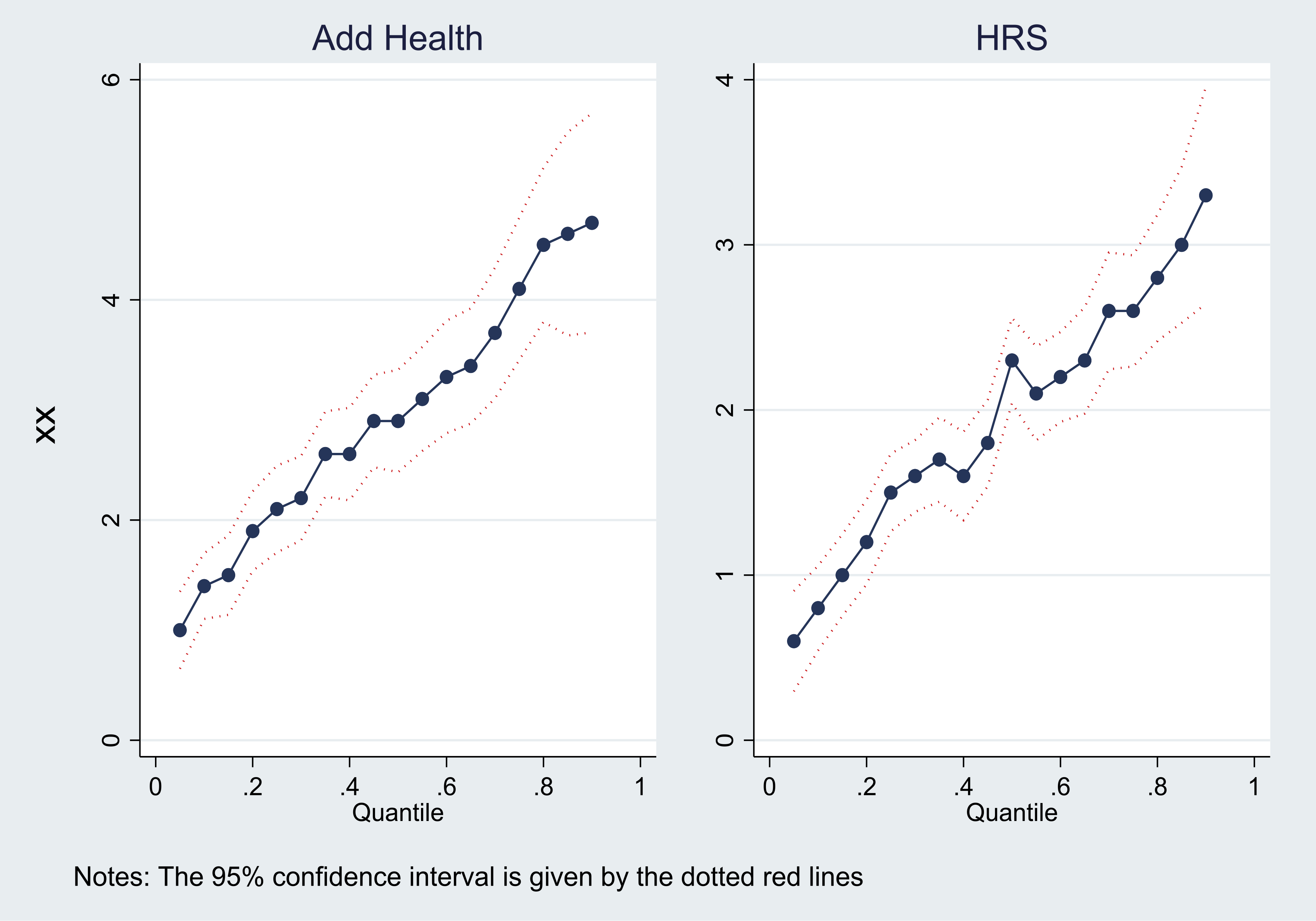
UNCONDITIONAL Quantile Treatment Effects of the Binary IV ON BMI

The IV estimates are presented in Table 4. All the IV estimates for the effect of BMI for young adults are statistically insignificant and relatively small in magnitude, suggesting that there is no causal effect of BMI on mental health. In comparison, the IV estimates for elderly individuals are statistically significant and comparably large in magnitude. For example, IV estimates in column 4 indicate that the effect of a 5 kg/m² increase in BMI is a 0.255 (20%) increase in the CES-D score, and a 3.57 percentage point (29%) increase in the probability of depression. There are no statistically significant gender differences. For comparison, Online Appendix Table 2 presents IV estimates using a binary variable equal to 1 if the BMI PGS is greater than 0 as the instrument, which are not substantially different from those in Table 4.

Table 4:

IV Estimates of the Effect of BMI on Mental Health in Young and Old Adults

	Add Health			HRS
	All	Women	Men	All	Women	Men
	(1)	(2)	(3)	(4)	(5)	(6)
A: CES-D Score
Outcome Mean	5.79	6.18	5.33	1.26	1.43	1.03
BMI	0.020 (.038)	0.019 (.054)	0.020 (.053)	0.051*** (.015)	0.053*** (.019)	0.046*** (.023)
Depression PGS	0.360*** (.086)	0.353*** (.125)	0.386 (.117)	0.128*** (.020)	0.122*** (.029)	0.138*** (.027)
Education PGS	−0.104 (.076)	−0.111 (.102)	−0.086 (.096)	−0.078*** (.021)	−0.088*** (.031)	−0.062*** (.029)
B: Depressed
Outcome Mean	0.15	0.17	0.12	0.12	0.14	0.09
BMI	0.003 (.003)	0.004 (.004)	0.001 (.004)	0.007*** (.003)	0.007** (.004)	0.007* (.004)
Depression PGS	0.022*** (.007)	0.024** (.010)	0.022 (.009)**	0.024*** (.006)	0.019*** (.005)	0.013** (.005)
Education PGS	−0.004 (.005)	−0.003 (.008)	−0.003 (.007)	−0.010 (.006)	−0.016*** (.006)	−0.006 (.005)
N	4928	2643	2285	8867	5104	3763

Notes: Add Health regressions in columns 1–3 control for age, age squared, gender, birth order, mother’s education, picture vocabulary score, and the first 20 ancestry-specific principal components of the genetic data. HRS regressions in columns 4–6 control for age, age squared, gender, mother’s education and the first 10 ancestry-specific principal components of the genetic data. Heteroscedasticity-robust standard errors in parentheses.

^***significant at 1%

^**significant at 5%

^*significant at 10%

It is important to note that the IV estimates appear to be overestimated when models do not control for the education and depression PGSs, which is consistent with DiPrete et al.’s (2018) argument that the inclusion of the outcome’s PGS may reduce the consequences of pleiotropy. More concretely, the change in the IV estimates occurs because the education and depression PGSs are correlated with the BMI PGS, which means that the instrument picks up some of the influence of these two PGSs when they are omitted.²¹ This point is illustrated in Table 5, which presents IV estimates that do not control for the education and depression PGSs. The IV estimates are considerably larger in the HRS when not adjusting for the education and depression PGSs, although the differences in coefficients are not statistically significant. For example, the effect of BMI on CES-D score (depression) when controlling for the PGSs in Table 4 column 4 is 0.051 (0.007). In contrast, the effect of BMI on CES-D (depression) when not controlling for the PGSs in Table 5 column 4 are 0.065 (0.009), reflecting an increase of 27% (29%). In Add Health, the IV estimates appear overestimated to a lesser extent. The effect of BMI on CES-D score when adjusting for the education and depression PGSs is 0.020 in Table 4 column 1. The corresponding IV estimate without controlling for the education and depression PGSs in Table 5 column 1 is 20% larger at 0.024. The IV estimates for depression in Tables 4 and 5 are the same.

Table 5:

IV Estimates of the Effect of BMI on Mental Health in Young and Old Adults without controlling for PGSs for depression and educational attainment

	Add Health			HRS
	All	Women	Men	All	Women	Men
	(1)	(2)	(3)	(4)	(5)	(6)
A: CES-D Score
Outcome Mean	5.79	6.18	5.33	1.26	1.43	1.03
BMI	0.024 (.037)	0.022 (.053)	0.026 (.052)	0.065*** (.014)	0.070*** (.019)	0.056*** (.019)
B: Depressed
Outcome Mean	0.15	0.17	0.12	0.12	0.14	0.09
BMI	0.003 (.003)	0.004 (.004)	0.001 (.004)	0.009*** (.003)	0.010*** (.003)	0.008*** (.004)
N	4928	2643	2285	8867	5104	3763

Notes: Add Health regressions in columns 1–3 control for age, age squared, gender, birth order, mother’s education, picture vocabulary score, and the first 20 ancestry-specific principal components of the genetic data. HRS regressions in columns 4–6 control for age, age squared, gender, mother’s education and the first 10 ancestry-specific principal components of the genetic data. Heteroscedasticity-robust standard errors in parentheses.

^***significant at 1%

^**significant at 5%

^*significant at 10%

Finally, we note that even with the inclusion of the depression and education PGSs, the BMI PGS may still violate the exclusion restriction assumption through other channels. Thus, to complement the evidence from the IV estimates, we employ the alternative approach of obtaining an upper bound for the average effect of BMI on mental health for the corresponding population.

4.3. Nevo & Rosen (2012) Bounds Estimates

In this section, we present evidence about the population ATE of BMI on mental health given by the parameter β in equation (1), by using the BMI PGS as a potentially imperfect IV based on the approach by Nevo & Rosen (2012) discussed in section 3.2. Recall that, since (i) our IV (BMI PGS) is positively correlated with the endogenous variable (BMI), and (ii) the IV and endogenous variable are assumed to be positively correlated with the error term u in equation (1) (see discussion in section 3.2), the bounding procedure yields an upper bound on the ATE (β).

Results for the CES-D score are presented in Table 6. Panel A shows results for young adults in Add Health. Columns 2 and 3 show the OLS and IV estimates from Tables 2 and 4, respectively. Column 4 shows the IV estimate using V(1) = σ_BMIPGS_BMI − 1σ_{PGS_BMI}BMI as the instrument, which is an intermediate step in the Nevo & Rosen procedure. The estimated upper bound on β under (A4)—that the instrument (PGS for BMI) has weakly the same direction of correlation with the error term u in equation (1) as the endogenous variable (BMI)—is given in column 5, and corresponds to the upper bound given in equation (2), which equals the min of the OLS and IV estimates. The estimated upper bound, while not able to rule out a null effect, indicates that the largest value of the ATE of BMI on the CES-D score for the population of young adults is 0.02. Based on this largest possible value for the effect, a 5 kg/m² increase in BMI would increase the average CES-D score in the population of young adults by at most a 0.1 unit (2%), suggesting that the average effect for young adults is, at most, small. Hence, in this case the estimated upper bound provides valuable information as it rules out plausible effects larger than 0.02. The upper endpoint of the 95% confidence interval on the bounded parameter is 0.052.²² Looking at the OLS estimate of β in equation (1), we see that it falls below the upper endpoint of the 95% confidence interval of the bounded parameter β. Since they both undertake statistical inference on the same parameter β (ATE), this implies that we cannot statistically rule out that the OLS estimate is unbiased for the true population average effect (β) using the estimated upper bound. The estimated upper bounds on β also suggest that there could be a gender difference in the effect of BMI on the CES-D score among young adults. In particular, for women, the estimated upper bound on β is consistent with a 5 kg/m² increase in BMI increasing the average CES-D score of young women by at most 2%. For men, the estimated upper bound is negative, although the upper endpoint of the 95% confidence interval on the bounded parameter β straddles zero, implying that a null effect is possible. Column 6 gives the estimated upper bounds on β when we add (A5)—that the instrument (PGI for BMI) is less correlated with the error term u in equation (1) than the endogenous variable (BMI). These bounds correspond to that in equation (3), which equals the min of the IV estimators using either PGS for BMI or V(1) as an instrument (see section 3.2 for details).These estimated upper bounds on β turn out to be not much different from those in column 5 for young adults, the main difference being that the upper endpoints of the 95% confidence interval on the bounded parameter β are somewhat larger.

Table 6:

OLS, IV and Upper Bounds Estimates for the Effect of BMI on CES-D Score

	Mean (1)	OLS (2)	IV (3)	IV(1) (4)	UB of β under (A4) (5)	UB of β under (A4 & A5) (6)
Panel A: Add health
All	5.79	0.028*** (.010)	0.020 (.038)	0.032** (.016)	0.020 [.052]	0.020 [.066]
Women	6.18	0.062*** (.014)	0.019 (.054)	0.075*** (.020)	0.019 [.094]	0.019 [.118]
Men	5.33	−0.028** (.014)	0.020 (.053)	−0.045* (.023)	−0.028 [−.003]	−0.027 [.010]
Panel B: HRS
All	1.26	0.029*** (.004)	0.051*** (.015)	0.022*** (.006)	0.029 [.037]	0.022 [.035]
Women	1.43	0.030*** (.005)	0.053*** (.019)	0.023*** (.008)	0.030 [.041]	.023 [.040]
Men	1.03	0.026*** (.006)	0.046*** (.023)	0.019** (.010)	0.026 [.041]	0.018 [.042]

Notes: Add Health regressions control for age, age squared, gender, birth order, mother’s education, picture vocabulary score, PGSs for depression and education, and the first 20 ancestry-specific principal components of the genetic data. HRS regressions control for age, age squared, gender, mother’s education, PGSs for depression and education, and the first 10 ancestry-specific principal components of the genetic data. Heteroscedasticity-robust standard errors in (.)

^***significant at 1%

^**significant at 5%

^*significant at 10%.

The Nevo & Rosen (2012) approach is implemented using the imperfectiv command in Stata. The upper endpoint of the 95% confidence interval on the bounded parameter is given in [.].

Results for elderly individuals in the HRS are given in panel B of Table 6. The estimated upper bound on the ATE (β) for the elderly population in column 5 equals 0.029, implying that for the elderly the average effect of a 5 kg/m² increase in BMI is, at most, an 12% increase in the CES-D score. Thus, this estimated upper bound on β is informative as it rules out plausible larger effects. Compared to the IV estimate (0.051), the estimated upper bound on β is about half as large. However, the lower endpoint of the 95% confidence interval of the IV estimate (note that its standard error is 0.015) is below the upper endpoint of the 95% confidence interval of the upper bound of β, making their difference non-statistically significant. Contrary to the young adult population, the estimated upper bounds on the corresponding ATE (β) for elderly women and men are very similar. Lastly, the estimated upper bounds on β that add (A5), shown in column 6 are somewhat smaller in magnitude, and yield very similar conclusions to the results in column 5.

Results for depression are shown in Table 7. In general, the patterns observed are similar to those documented in Table 6 for the CES-D score, although the differences in estimated upper bounds on β between young adults and the elderly are less pronounced. Looking at the estimated bounds on β under (A4) in column 5, for the population of young adults the largest possible value for the ATE indicates that a 5 kg/m² increase in BMI increases the probability of experiencing depression by at most 7%. For the elderly population, the estimated upper bound on β indicates a corresponding increase of at most 13% in the probability of experiencing depression. As before, the estimated upper bounds on β are able to rule out plausible larger effects.

Table 7:

OLS, IV and Upper Bounds Estimates for the Effect of BMI on Depression

	Mean (1)	OLS (2)	IV (3)	IV(1) (4)	UB of β under (A4) (5)	UB of β (A4 & A5) (6)
Panel A: Add health
All	0.15	0.002*** (.001)	0.003 (.003)	0.002 (.001)	0.002 [.004]	0.002 [.004]
Women	0.17	0.004*** (.001)	0.004 (.004)	0.004** (.002)	0.004 [.006]	0.004 [.0007]
Men	0.12	−0.002 (.0010)	−0.001 (.004)	−0.002 (.002)	−0.002 [.001]	−0.001 [.002]
Panel B: HRS
All	0.12	0.003*** (.001)	0.007*** (.003)	0.002** (.001)	0.003 [.005]	0.002 [.005]
Women	0.14	0.004*** (.001)	0.007** (.004)	0.003* (.001)	0.004 [.006]	.003 [.006]
Men	0.09	0.003*** (.001)	0.007* (.004)	0.002 (.002)	0.003 [.005]	0.001 [.006]

Notes: Add Health regressions control for age, age squared, gender, birth order, mother’s education, picture vocabulary score, PGSs for depression and education, and the first 20 ancestry-specific principal components of the genetic data. HRS regressions control for age, age squared, gender, mother’s education, PGSs for depression and education, and the first 10 ancestry-specific principal components of the genetic data. Heteroscedasticity-robust standard errors in (.)

^***significant at 1%

^**significant at 5%

^*significant at 10%.

The Nevo & Rosen (2012) approach is implemented using the imperfectiv command in Stata. The upper endpoint of the 95% confidence interval on the bounded parameter is given in [.].

Overall, the results from employing the Nevo & Rosen (2012) bounds can be summarized as follows. First, the estimated upper bounds on β for the population of young adults are consistent with the finding based on the IV estimates that the effect of BMI on mental health is at most small and arguably economically insignificant for young adults. Second, the estimated upper bounds on β are suggestive of economically significant effects of BMI on mental health for the elderly population. Lastly, the estimated upper bounds on β for both young adults and the elderly rule out plausible large effects (especially for young adults), and are thus informative.

4.4. Other Analyses

4.4.1. Obesity and Extreme Obesity

Our main analyses focus on BMI rather than obesity (BMI≥30) because the instrument affects mental health through variation in BMI across the BMI distribution, not just incidence in obesity. Nevertheless, since the effect of BMI on mental health could be nonlinear, we have analyzed the effect of obesity and extreme obesity (BMI≥40) on mental health in Online Appendix Table A3. The results for obesity and extreme obesity are qualitatively similar to the BMI results. For young adults, the IV estimates show no statistically significant difference in mental health by obesity or extreme obesity status. We note that the IV estimates in Online Appendix Table A3 are somewhat large (although smaller than the OLS associations) but imprecisely estimated. This is suggestive of the effect of BMI on mental health for young adults possibly being nonlinear; however, there is not enough precision in this sample to have statistical confidence that the effects are non-zero. For elderly individuals, the IV estimates indicate that there are large statistically significant differences in mental health by obesity and extreme obesity status. For instance, obese individuals have a higher CES-D score by 0.705 units (56% relative to the sample mean), and are 10.2 percentage points (85% relative to the sample mean) more likely to be depressed than non-obese individuals. Noteworthy is that, for elderly individuals, when considering obesity and extreme obesity status, the IV estimates are generally larger and remain statistically significant, which is consistent with the notion that the effect identified by the IV estimates presented in section 4.2 capture the effect of BMI on mental health mostly for complier individuals on the upper part of the BMI distribution.²³

4.4.2. Reverse Causality and Mortality Attrition

We have also examined whether the findings for elderly individuals are influenced by (i) reverse causality, and (ii) mortality attrition. To assess the influence of reverse causality, we estimated the effect of mental health on BMI using the PGS for depression as the IV. Unlike the PGS for BMI, which predicts both BMI (first-stage effect) and mental health (reduced-form effect), the PGS for depression only predicts mental health (second-stage effect). Online Appendix Table A4 shows OLS and IV estimates using the HRS sample. While OLS estimates are positive and statistically significant, IV estimates are statistically insignificant, which provides suggestive evidence that reverse causality is unlikely to be driving our results.

A second potential concern is that our estimates could be affected by mortality attrition, as genetic data is only available for HRS respondents who have survived until 2006. A key concern is that mortality attrition changes the composition of the elderly sample in a way that is related to body mass and mental health. The direction of the potential resulting bias is not entirely clear. There is evidence documenting that mortality attrition in the HRS results in a sample with better self-reported health, less reported medical conditions, and higher socioeconomic status (e.g., Zajacova & Burgard, 2013). In light of this sample selection caused by mortality attrition, we conjecture that the potential resulting bias can be an underestimation of the true effect if the causal link between BMI and mental health is muted for generally healthier individuals. Therefore, as a robustness check, we weighted the IV regressions with the inverse of the probability of surviving until 2006. The probabilities are the predicted values from a logit regression where the dependent variable is an indicator for being alive in 2006 on basic demographics (year of birth, gender), health (ever smoked, ever had diabetes, ever had heart disease, average BMI up to 2004, average CES-D score up to 2004, average self-reported health up to 2004), and socioeconomic variables (years of education, mother’s education). This exercise assumes that, conditional on the previous covariates, the potential effect of mortality attrition on our estimates can be ignored. As shown in Online Appendix Table A5, the IV estimates are qualitatively similar to those presented in Table 4.²⁴ The one exception is that the effect of BMI on depression for women becomes statistically insignificant. While not definitive, this exercise suggests that our results are not dramatically affected by mortality attrition.

4.4.3. Exploration of Some Mechanisms

In general, our analysis in sections 4.2 and 4.3 suggests that there are economically and statistically significant effects of BMI on mental health (as measured by the CES-D score and depression) for the elderly, but not for young adults. For the latter group, this result is consistent with previous findings in the literature. For example, Hung et a. (2014) find no effect of BMI on the probability of having a major depressive disorder using data from RADIANT, while Willage (2018) also finds no effect of BMI on the CES-D score using the sibling sample of the Add Health.²⁵

As discussed in the introduction, BMI is hypothesized to affect mental health through various channels, including social stigma (which can lead to perceived or actual discrimination), body-image dissatisfaction, poor health, functional limitations, and biological processes (among others). To understand our findings, in this section we analyze the effect of BMI on some of these potential mechanisms through which BMI may affect mental health, using information available in the Add Health and the HRS. Importantly, the relevance of different mechanisms—in terms of both how much BMI affects a mechanism and how much that mechanism in turn affects mental health—may be different for young adults and the elderly. Based on prior literature (e.g., Himes 2000; Willage 2018), we hypothesize that the more relevant mechanisms for young adults are social stigma and self-image, while for the elderly are functional limitations and poor health, among others.

At the outset, it is important to note that the analysis below only looks at the effect of BMI on potential mechanisms. Thus, finding a statistically significant effect for a potential mechanism does not imply that such variable is indeed a mechanism. To statistically show that such a variable is a mechanism, one would also need to show that the effect of BMI on the potential mechanism in turn affects mental health, which would require a formal causal mediation analysis (e.g., Huber 2019). Given that causal mediation typically requires considerably stronger assumptions than those necessary to estimate “total” average effects (e.g., Flores & Flores-Lagunes 2009; Huber 2019), we follow prior literature and focus on estimating the effect of the treatment (in our case BMI) on potential mechanisms (e.g., Currie and Moretti 2003; Willage 2008).

Online Appendix Table A6 presents estimates (OLS and IV) of the effect of BMI on the following potential mechanisms for young adults: (i) the probability of being in very good/excellent health, (ii) the probability that the interviewer rates the respondent as being very attractive (which is likely to capture social stigma), and (iii) the probability that the respondent rates him/herself as being very attractive. In panel A, we find evidence that BMI decreases the probability of self-reporting very good/excellent health. The IV estimate in column 3 suggests that a 5 kg/m² increase in BMI decreases the likelihood of reporting being in very good or excellent health by 7 percentage points (11% relative to the sample mean). This estimated effect is present in both women and men. The estimates in panel B show that there is a relatively large effect of BMI on perceived attractiveness by the interviewer for women. For example, according to the IV estimate in column 3, the effect of a 5 kg/m² increase in BMI decreases the probability of women being viewed very attractive by 8 percentage points (73%). In panel C, the IV estimates show that there is no strong effect of BMI on self-reported attractiveness. In fact, the IV estimate for the sample implies a surprising positive relationship between BMI and self-reported attractiveness—which is only marginally statistically significant—that is driven by men. For men, the IV estimate is statistically significant and implies that a 5 kg/m² increase in BMI increases the probability of judging oneself very attractive by 5 percentage points (50%). Overall, for young adults, BMI has a statistically significant effect on potential mechanisms for the effect of BMI on mental health. However, given our results from the previous section that BMI does not statistically significantly affect mental health for young adults, we interpret these findings as suggesting that those potential mechanisms are not strong enough to produce a detectable effect of BMI on mental health, as measured using CES-D score, depression, and suicidal ideation (see footnote 28).

For the elderly, Online Appendix Table A7 shows results for the effect of BMI on the (i) probability of being in very good/excellent health, (ii) probability of engaging in vigorous exercise more than once per week, and (iii) probability of reporting that health limits at least one daily activity. Similar to young adults, we find that there are large effects of BMI on self-reported health for elderly individuals. The IV estimate in column 3 of panel A suggests that a 5 kg/m² increase in BMI decreases the likelihood of reporting being in very good or excellent health by 9.5 percentage points (20%). In panel B we see that, according to the IV estimate, the effect of a 5 kg/m² increase in BMI is a 6.5 percentage point (25%) decrease in the likelihood of engaging in vigorous exercise more than once per week. Looking at panel C, the IV estimate suggests that a 5 kg/m² increase in BMI increases the likelihood of reporting that health limits at least one daily activity by 5 percentage points (42%). We interpret these findings as suggesting that functional limitations and health concerns are among the mechanisms through which BMI may affect mental health for the elderly. Contrary to young adults, for the elderly these mechanisms appear strong enough to significantly impact their mental health given the reported statistically significant effects of BMI on mental health for this group in sections 4.2 and 4.3.

5. Conclusion

We study the effect of BMI on mental health for young adults in Add Health and elderly individuals in the HRS. To account for confounding due to unobserved factors and reverse causality, we first take the same approach as previous studies (Hung et al. 2014; Jokel et al. 2012; Tyrrell et al. 2018; Walter et al. 2015; Willage 2018) and use a PGS for BMI as an IV. However, unlike previous studies, we attempt to address the possible violation of the exclusion restriction assumption due to pleiotropy by using PGSs for depression and education to control for the genetic predisposition to poor mental health and innate ability. We also contribute to this literature by analyzing effects of the IV on the BMI quantiles to help characterize the latent subpopulation for which the IV estimates identify an effect. We document that IV estimates capture the effect of BMI on mental health for (complier) individuals in the upper quantiles of the BMI distribution. As a second, complementary analysis, we estimate an upper bound on the ATE for the corresponding population of young adults or the elderly. We use the bounding approach of Nevo & Rosen (2012), which has not been used in this context as far as we are aware. The attractiveness of this approach is that it allows the PGS for BMI to be an “imperfect” instrument that may not satisfy the exclusion restriction.

For young adults, the IV estimates indicate that there is no statistically significant effect of BMI on mental health. The estimated upper bounds on the ATE are consistent with the notion that the effect of BMI on mental health for young adults is at most small and economically insignificant. The results for young adults are consistent with those in Willage (2018). In contrast to young adults, the IV estimates for elderly individuals are statistically and economically significant. They indicate that a 5 kg/m² increase in BMI (a difference equivalent to moving from overweight to obese) increases the CES-D score by 20%, and the likelihood of depression by 29%. We find no statistically significant gender differences in the IV estimates. The estimated upper bounds on the ATE are consistent with the IV estimates in that they are also suggestive of large and economically significant effects of BMI on mental health for the elderly population. Finally, our analysis of the effect of BMI on potential mechanisms through which BMI may affect mental health suggests that functional limitations and health concerns may be important mechanisms for the elderly. However, analyzing only the effect of BMI on potential mechanisms (a common practice in the literature) falls short on determining the causality of the mechanisms and quantifying their importance, as this would require the use of a formal causal mediation framework (e.g., Huber 2019). We leave the task of formally applying causal mediation in this setting for further research.

Overall, our paper provides new insights regarding the effect of BMI on mental health that can be valuable from a policy perspective, for example, when considering the costs of the ongoing obesity epidemic in the United States or the benefits of policies that have been implemented to fight it. First, our analysis suggests that the IV estimates of the kind used in this paper likely reflect a weighted average of effects of BMI on mental health for complier individuals on the upper quantiles of the BMI distribution. This is a critical consideration in using this kind of IV estimates for policy purposes. For example, since the compliers in the upper quantiles of the BMI distribution are a subset of individuals in those upper quantiles, our estimates suggest that policies targeting the upper quantiles of the BMI distribution (e.g., obesity or extreme obesity) would have significant effects on mental health at least for a subset of the individuals in those upper quantiles.²⁶ Second, taken together, our results from the IV estimates and the estimated bounds on the ATE suggest that the effect of BMI on mental health is economically significant for the elderly, but not for young adults.²⁷ Hence, for example, if a policy were to affect the BMI of different age groups in a similar way, our results would suggest that the indirect benefits of such policies in terms of improved mental health are likely larger for the elderly than for young adults. Third, our analysis of potential mechanisms through which BMI may affect mental health suggests that, for the elderly, functional limitations and health concerns are potentially important mechanisms. Taken at face value, this suggests, for example, that policies targeted at reducing the functional limitations of the elderly (e.g., by subsidizing appropriate medical equipment or human assistance) may ameliorate the negative effects of BMI on the mental health for them.

There are some limitations with our paper. For instance, we focus on European ancestry individuals because GWASs are mostly conducted on European descent populations. This means that PGSs for other ethnic groups may not have the same predictive power (Martin et al. 2017). We also do not look at the effect of BMI on mental health in midlife, which may differ from the effect found for young adults and elderly individuals.

References

- Angrist JD, & Imbens GW (1995). Two-stage least squares estimation of average causal effects in models with variable treatment intensity. Journal of the American Statistical Association, 90(430), 431–442. [Google Scholar]
- Angrist JD, Imbens GW, & Rubin DB (1996). Identification of causal effects using instrumental variables. Journal of the American statistical Association, 91(434), 444–455. [Google Scholar]
- Beck AT, Ward CH, Mendelson M, Mock J, & Erbaugh J (1961). An inventory for measuring depression. Archives of General Psychiatry, 4(6), 561–571. [DOI] [PubMed] [Google Scholar]
- Beck AT, & Steer RA (1993). Beck Depression Inventory manual. San Antonio, TX: Harcourt. [Google Scholar]
- Bonanno A, Bimbo F, Cleary R, & Castellari E (2018). Food labels and adult BMI in Italy–An unconditional quantile regression approach. Food Policy, 74, 199–211. [Google Scholar]
- Böckerman P, Cawley J, Viinikainen J, Lehtimäki T, Rovio S, Seppälä I, … & Raitakari O (2019). The effect of weight on labor market outcomes: An application of genetic instrumental variables. Health Economics, 28(1), 65–77. [DOI] [PMC free article] [PubMed] [Google Scholar]
- Brunello G, & d’Hombres B (2007). Does body weight affect wages?: Evidence from Europe. Economics & Human Biology, 5(1), 1–19. [DOI] [PubMed] [Google Scholar]
- Cardon LR, & Palmer LJ (2003). Population stratification and spurious allelic association. The Lancet, 361(9357), 598–604. [DOI] [PubMed] [Google Scholar]
- Carpenter KM, Hasin DS, Allison DB, & Faith MS (2000). Relationships between obesity and DSM-IV major depressive disorder, suicide ideation, and suicide attempts: results from a general population study. American Journal of Public Health, 90(2), 251. [DOI] [PMC free article] [PubMed] [Google Scholar]
- Chernozhukov V, Lee S, & Rosen A (2013). Intersection bounds: Estimation and inference. Econometrica, 81(2), 667–737. [Google Scholar]
- Crisp AH, Queenan M, Sittampaln Y, & Harris G (1980). ‘Jolly fat’ revisited. Journal of Psychosomatic Research, 24(5), 233–241. [DOI] [PubMed] [Google Scholar]
- Currie J, & Moretti E (2003). Mother’s education and the intergenerational transmission of human capital: Evidence from college openings. Quarterly Journal of Economics, 118(4), 1495–1532. [Google Scholar]
- DiPrete T, Burik CAP & Koellinger PD. (2018). Genetic instrumental variable regression: Explaining socioeconomic and health outcomes in nonexperimental data. Proceedings of the National Academy of Sciences, 115, E4970–E4979. [DOI] [PMC free article] [PubMed] [Google Scholar]
- Firpo S (2007). Efficient semiparametric estimation of quantile treatment effects. Econometrica, 75(1), 259–276. [Google Scholar]
- Fletcher JM (2018). Economics and Genomics. In Oxford Research Encyclopedia of Economics and Finance. [Google Scholar]
- Flores CA & Flores-Lagunes A (2009). Identification and estimation of causal mechanisms and net effects of a treatment under unconfoundedness. IZA DP No. 4237. [Google Scholar]
- Fryar CD, Kruszon-Moran D, Gu Q, Ogden CL (2018). Mean body weight, height, waist circumference, and body mass index among adults: United States, 1999–2000 through 2015–2016. National Health Statistics Reports; no 122. Hyattsville, MD: National Center for Health Statistics. [PubMed] [Google Scholar]
- Gregor MF, & Hotamisligil GS (2011). Inflammatory mechanisms in obesity. Annual Review of Immunology, 29, 415–445. [DOI] [PubMed] [Google Scholar]
- Greve Jane. “Obesity and labor market outcomes in Denmark.” Economics & Human Biology 6, no. 3 (2008): 350–362. [DOI] [PubMed] [Google Scholar]
- Ha H, Han C, & Kim B (2017). Can Obesity Cause Depression? A Pseudo-panel Analysis. Journal of Preventive Medicine and Public Health, 50(4), 262. [DOI] [PMC free article] [PubMed] [Google Scholar]
- Han E, & Powell LM (2013). Fast food prices and adult body weight outcomes: evidence based on longitudinal quantile regression models. Contemporary Economic Policy, 31(3), 528–536. [Google Scholar]
- Himes CL (2000). Obesity, disease, and functional limitation in later life. Demography, 37(1), 73–82. [PubMed] [Google Scholar]
- Huber M (2019). A review of causal mediation analysis for assessing direct and indirect treatment effects. SES Working Paper 500, University of Fribourg. [Google Scholar]
- Hung CF, Rivera M, Craddock N, Owen MJ, Gill M, Korszun A, … & Rietschel M (2014). Relationship between obesity and the risk of clinically significant depression: Mendelian randomisation study. The British Journal of Psychiatry, 205(1), 24–28. [DOI] [PMC free article] [PubMed] [Google Scholar]
- Imbens G (2004). Nonparametric estimation of average treatment effects under exogeneity: A review. Review of Economics and Statistics, 86(1), 4–29. [Google Scholar]
- Imbens G, & Angrist J (1994). Identification and estimation of local average treatment effects. Econometrica, 62(2), 467–475. [Google Scholar]
- Insel TR (2008). Assessing the economic costs of serious mental illness. The American Journal of Psychiatry, 165(6), 663–665. [DOI] [PubMed] [Google Scholar]
- Jokela M, Elovainio M, Keltikangas-Järvinen L, Batty GD, Hintsanen M, Seppälä I, … & Kivimäki M (2012). Body mass index and depressive symptoms: instrumental-variables regression with genetic risk score. Genes, Brain and Behavior, 11(8), 942–948. [DOI] [PubMed] [Google Scholar]
- Kessler RC, Mickelson KD, & Williams DR (1999). The prevalence, distribution, and mental health correlates of perceived discrimination in the United States. Journal of Health and Social Behavior, 40, 208–230. [PubMed] [Google Scholar]
- Lee JJ, Wedow R, Okbay A, Kong E, Maghzian O, Zacher M, … & Fontana MA (2018). Gene discovery and polygenic prediction from a genome-wide association study of educational attainment in 1.1 million individuals. Nature Genetics, 50(8), 1112. [DOI] [PMC free article] [PubMed] [Google Scholar]
- Locke AE, Kahali B, Berndt SI, Justice AE, Pers TH, Day FR, … & Croteau-Chonka DC (2015). Genetic studies of body mass index yield new insights for obesity biology. Nature, 518(7538), 197. [DOI] [PMC free article] [PubMed] [Google Scholar]
- Luppino FS, de Wit LM, Bouvy PF, Stijnen T, Cuijpers P, Penninx BW, & Zitman FG (2010). Overweight, obesity, and depression: a systematic review and meta-analysis of longitudinal studies. Archives of General Psychiatry, 67(3), 220–229. [DOI] [PubMed] [Google Scholar]
- Markowitz S, Friedman MA, & Arent SM (2008). Understanding the relation between obesity and depression: causal mechanisms and implications for treatment. Clinical Psychology: Science and Practice, 15(1), 1–20. [Google Scholar]
- Martin AR, Gignoux CR, Walters RK, Wojcik GL, Neale BM, Gravel S, … & Kenny EE (2017). Human demographic history impacts genetic risk prediction across diverse populations. The American Journal of Human Genetics, 100(4), 635–649. [DOI] [PMC free article] [PubMed] [Google Scholar]
- Miller AH, & Raison CL (2016). The role of inflammation in depression: from evolutionary imperative to modern treatment target. Nature Reviews Immunology, 16(1), 22. [DOI] [PMC free article] [PubMed] [Google Scholar]
- Morris S (2007). The impact of obesity on employment. Labour Economics, 14(3), 413–433. [Google Scholar]
- National Alliance on Mental Illness “Mental Health By The Numbers”. Retrieved from: https://www.nami.org/learn-more/mental-health-by-the-numbers
- National Institute of Mental Health, “Mental health Statistics”. Retrieved from: https://www.nimh.nih.gov/health/statistics/index.shtml
- Nevo A, & Rosen AM (2012). Identification with imperfect instruments. Review of Economics and Statistics, 94(3), 659–671. [Google Scholar]
- Okbay A, Baselmans BM, De Neve JE, Turley P, Nivard MG, Fontana MA, … & Gratten J (2016). Genetic variants associated with subjective well-being, depressive symptoms, and neuroticism identified through genome-wide analyses. Nature Genetics, 48(6), 624. [DOI] [PMC free article] [PubMed] [Google Scholar]
- Palinkas LA, Wingard DL, & Barrett-Connor E (1996). Depressive symptoms in overweight and obese older adults: a test of the “jolly fat” hypothesis. Journal of Psychosomatic Research, 40(1), 59–66. [DOI] [PubMed] [Google Scholar]
- Paolucci EM, Loukov D, Bowdish DM, & Heisz JJ (2018). Exercise reduces depression and inflammation but intensity matters. Biological Psychology, 133, 79–84. [DOI] [PubMed] [Google Scholar]
- Price AL, Patterson NJ, Plenge RM, Weinblatt ME, Shadick NA, & Reich D (2006). Principal components analysis corrects for stratification in genome-wide association studies. Nature Genetics, 38(8), 904–909. [DOI] [PubMed] [Google Scholar]
- Puhl RM, & Heuer CA (2010). Obesity stigma: important considerations for public health. American Journal of Public Health, 100(6), 1019–1028. [DOI] [PMC free article] [PubMed] [Google Scholar]
- Radloff LS (1977). The CES-D scale: A self-report depression scale for research in the general population. Applied Psychological Measurement, 1(3), 385–401. [Google Scholar]
- Roberts RE, Kaplan GA, Shema SJ, & Strawbridge WJ (2000). Are the obese at greater risk for depression?. American Journal of Epidemiology, 152(2), 163–170. [DOI] [PubMed] [Google Scholar]
- Rosen-Reynoso M, Alegría M, Chen CN, Laderman M, & Roberts R (2011). The relationship between obesity and psychiatric disorders across ethnic and racial minority groups in the United States. Eating Behaviors, 12(1), 1–8. [DOI] [PMC free article] [PubMed] [Google Scholar]
- Scott KM, McGee MA, Wells JE, & Browne MAO (2008). Obesity and mental disorders in the adult general population. Journal of Psychosomatic Research, 64(1), 97–105. [DOI] [PubMed] [Google Scholar]
- Simon GE, Von Korff M, Saunders K, Miglioretti DL, Crane PK, Van Belle G, & Kessler RC (2006). Association between obesity and psychiatric disorders in the US adult population. Archives of General Psychiatry, 63(7), 824–830. [DOI] [PMC free article] [PubMed] [Google Scholar]
- Skorikov VB & Vandervoort DJ (2003). Relationships between the underlying constructs of the beck depression inventory and the center for epidemiological studies depression scale. Educational and Psychological Measurement, 63(2), 319–335. [Google Scholar]
- Speliotes EK, Willer CJ, Berndt SI, Monda KL, Thorleifsson G, Jackson AU, … & Randall JC (2010). Association analyses of 249,796 individuals reveal 18 new loci associated with body mass index. Nature Genetics, 42(11), 937. [DOI] [PMC free article] [PubMed] [Google Scholar]
- Steffick DE (2000). Documentation of Affective Functioning Measures in the Health and Retirement Study (http://hrsonline.isr.umich.edu/sitedocs/userg/dr-005.pdf).
- Substance Abuse and Mental Health Services Administration (2016). Behavioral Health Spending and Use Accounts, 1986–2014. HHS Publication No. SMA-16–4975. [PubMed]
- Suglia SF, Demmer RT, Wahi R, Keyes KM, & Koenen KC (2016). Depressive symptoms during adolescence and young adulthood and the development of type 2 diabetes mellitus. American Journal of Epidemiology, 183(4), 269–276. [DOI] [PMC free article] [PubMed] [Google Scholar]
- Tyrrell J, Mulugeta A, Wood AR, Beaumont RN, Tuke MA, Jones SE, … & Hyppönen E, (2018). Using genetics to understand the causal influence of higher BMI on depression. International Journal of Epidemiology, dyy223, 1–15. [DOI] [PMC free article] [PubMed] [Google Scholar]
- van Kippersluis H, & Rietveld C (2018). Pleiotropy-robust Mendelian Randomization. International Journal of Epidemiology, 47, 1279–1288. [DOI] [PMC free article] [PubMed] [Google Scholar]
- von Hinke S, Smith GD, Lawlor DA, Propper C, & Windmeijer F (2016). Genetic markers as instrumental variables. Journal of Health Economics, 45, 131–148. [DOI] [PMC free article] [PubMed] [Google Scholar]
- Walter S, Kubzansky LD, Koenen KC, Liang L, Tchetgen Tchetgen EJ, Cornelis MC, … & Glymour MM (2015). Revisiting mendelian randomization studies of the effect of body mass index on depression. American Journal of Medical Genetics Part B: Neuropsychiatric Genetics, 168(2), 108–115. [DOI] [PMC free article] [PubMed] [Google Scholar]
- Ware EB, Schmitz LL, Faul JD, Gard A, Mitchell C, Smith JA, … & Kardia SL (2017). Heterogeneity in polygenic scores for common human traits. BioRxiv, 106062. [Google Scholar]
- Willage B (2018). The effect of weight on mental health: New evidence using genetic IVs. Journal of Health Economics, 57, 113–130. [DOI] [PMC free article] [PubMed] [Google Scholar]
- Wehby GL, & Courtemanche CJ (2012). The heterogeneity of the cigarette price effect on body mass index. Journal of Health Economics, 31(5), 719–729. [DOI] [PMC free article] [PubMed] [Google Scholar]
- Wray NR, Ripke S, Mattheisen M, Trzaskowski M, Byrne EM, Abdellaoui A, … & Bacanu SA (2018). Genome-wide association analyses identify 44 risk variants and refine the genetic architecture of major depression. Nature Genetics, 50(5), 668. [DOI] [PMC free article] [PubMed] [Google Scholar]
- Zajacova A & Burgard S (2013). Healthier, wealthier, and wiser: A demonstration of compositional changes in aging cohorts due to selective mortality. Population Research and Policy Review, 32(3), 311–324. [DOI] [PMC free article] [PubMed] [Google Scholar]
- Zhao G, Ford ES, Dhingra S, Li C, Strine TW, & Mokdad AH (2009). Depression and anxiety among US adults: associations with body mass index. International Journal of Obesity, 33(2), 257. [DOI] [PubMed] [Google Scholar]
Associated Data
This section collects any data citations, data availability statements, or supplementary materials included in this article.