TA-Net: Topology-Aware Network for Gland Segmentation

Abstract

Gland segmentation is a critical step to quantitatively assess the morphology of glands in histopathology image analysis. However, it is challenging to separate densely clustered glands accurately. Existing deep learning-based approaches attempted to use contour-based techniques to alleviate this issue but only achieved limited success. To address this challenge, we propose a novel topology-aware network (TA-Net) to accurately separate densely clustered and severely deformed glands. The proposed TA-Net has a multitask learning architecture and enhances the generalization of gland segmentation by learning shared representation from two tasks: instance segmentation and gland topology estimation. The proposed topology loss computes gland topology using gland skeletons and markers. It drives the network to generate segmentation results that comply with the true gland topology. We validate the proposed approach on the GlaS and CRAG datasets using three quantitative metrics, F1-score, object-level Dice coefficient, and object-level Hausdorff distance. Extensive experiments demonstrate that TA-Net achieves state-of-the-art performance on the two datasets. TA-Net outperforms other approaches in the presence of densely clustered glands.

1. Introduction

In histopathology image analysis, evaluating gland morphology is crucial to determine stages of several cancers, e.g., colon cancer [11], breast cancer [3], and prostate cancer [16]. Conventionally, pathologists examine gland morphology to assess the malignancy degree using microscopes; and the whole process is time-consuming, expensive, and prone to human errors. Recently, with the availability of whole slide images (WSI), digital pathology has been achieving popularity by developing computational tools to aid routine tasks. Automatic and accurate gland segmentation is often required before calculating gland morphology. However, the task is challenging due to the large morphological differences among glands and large number of clustered glands (Figure. 1).

Figure 1.

Hematoxylin and Eosin (H&E) stained histopathology images with labeled (yellow contours) glands. The first row shows healthy glands, the second row shows malignant glands. Noted that the malignant glands are close their neighboring glands and appear in deformed shapes.

Early approaches for gland segmentation focused on applying knowledge of glandular structures, e.g., morphology-based methods [19, 21], and graph-based methods [30, 9]. These methods achieved promising performance on low-grade adenocarcinoma; but they failed in many malignant cases. Malignant glands continue to grow and invade the adjacent tissues or metastasize (Figure 1); therefore, they cluster densely and their shapes deform severely in histopthology images. Recently, deep learning-based methods provide state-of-the-art performance in many computer vision tasks [1, 6] and biomedical image analysis tasks [24]. Chen et al. [5] proposed an FCN-based multitask learning network to generate gland regions and contours simultaneously. The complementary contour information helped separate clustered glands. Xu et al. [33] developed a deep three-channel network (instance, contour, and location) to jointly separate the clustered glands. Graham et al. [12] proposed the MILD-Net that utilized both instance and contour segmentation; and MILD-Net also involved multi-level aggregation, atrous spatial pyramid pooling block, and dilated convolutional design. Qu et al. [22] proposed a full-resolutional network that outputs three-class probability maps (instance, contour and background). The strategy shared by all the above methods is to use gland contour information to separate clustered glands. However, these approaches achieved limited success. A segmentation example of densely clustered glands is shown in Figure. 2, SegNet, DCAN, and MicroNet failed to separate close glands.

Figure 2.

A segmentation example of densely clustered glands. Colors are used to differentiate different glands. The white dash rectangles highlight the poorly-separated glands.

Three major challenges exist in gland segmentation using contour information: 1) The contour strategy fails when glands are densely clustered, because overlapped glands share contour sections. Usually, in a glandular structure, epithelial nuclei form a gland border. In practice, digital WSI scanner flattens gland tissues into a near two-dimensional histopathology slice, and two or multiple glands cluster together will not have a regular and clear epithelial nuclei border. Note the red arrow in Figure. 3(a), the clustered regions do not have regular epithelial nuclei. 2)The coarse annotations of the contours introduce noise and reduce the effectiveness of the contour strategy. A gland tissue in a 20 × magnification could be 1k × 1k pixels wide and height, and it is difficult to annotate all contour pixels correctly. Existing datasets in the literature still have many annotation issue (Figure. 3(b)). 3) It is difficult to identify the contours of malignant glands accurately. Because malignant glands continue to grow and become deformed. their components appear distorted. The green arrows in Figure 3(c) indicate the distorted boundary of a malignant gland.

Figure 3.

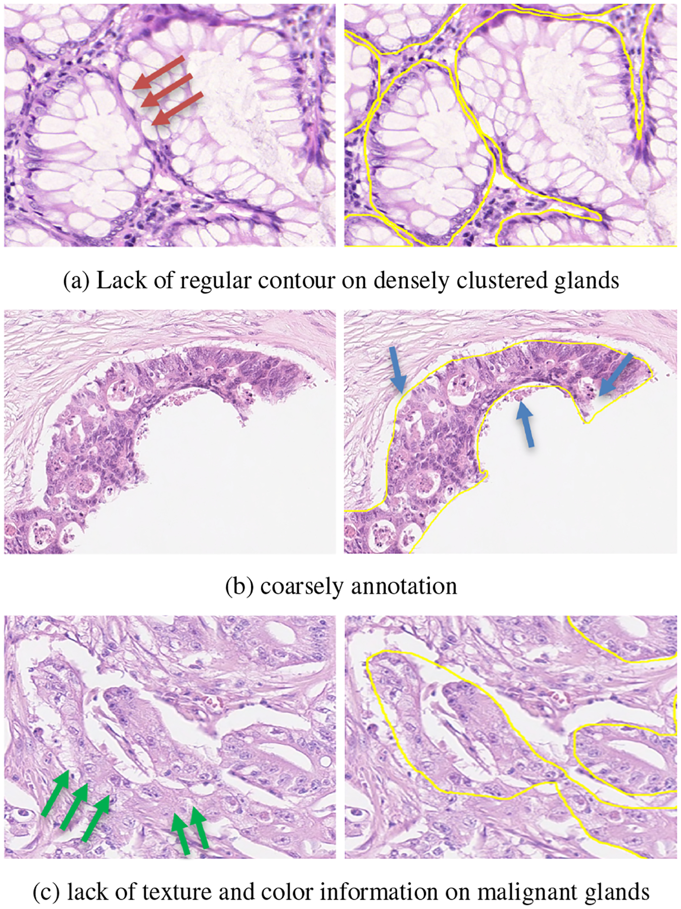
Issues of segmenting densely clustered glands by using a gland contour annotation. Left column shows the histopathology image patches; right column shows the image patches with the labeled gland contours (yellow).

In this paper, we introduce a new strategy that utilizes gland topology to separate densely clustered glands. The gland topology is characterized by the gland’s topological skeleton, which differentiates clustered glands better than gland contours. Furthermore, the gland topology is more reliable than contours in the presence of noisy annotations. This work has two major contributions: 1) we propose a topology-aware network that learns shared representation for simultaneously instance segmentation and gland topology estimation. The topology branch of the network predicts the Medial Axis [4] distance map to describe gland topology. 2) We propose a new topology loss by using the Medial Axis distance map and gland markers. The loss penalizes the topology difference between segmented glands and the true glands, which forces the network to generate segmentation results that adhere to the gland topology.

2. Related Work

2.1. Histopathology Gland Segmentation

Histopathology gland segmentation aims to segment the gland tissue from the Hematoxylin & Eosin (H&E) stained histopathology image. Recently, deep learning (DL)-based method successfully demonstrate the robustness and efficiency in the literature. Raza et al. [23] proposed the MicroNet that inputs the multiple resolutions of images patches at different down-sampling stages for better localization and context information and back-propagates the results by using multi-resolution outputs. Ding et al. [8] proposed a multi-scale Fully convolutional network to extract different receptive field features at different convolutional layers. These studies, as well as those described in the previous section [5, 33, 12], build up a deep architecture for segmenting the gland instance and contours. Yan et al. [34] proposed a shape-aware adversarial learning network that integrates a deep adversarial network and a shape-preserve loss. Qu et al. [22] proposed a spatial loss for recognizing the glands. The proposed loss placed a spatial constraint on the boundary pixels and forced the network to learn gland shapes.

2.2. Topology Aware Networks

Different Topology aware networks have been proposed in various natural image segmentation [7, 10, 17] and biomedical image segmentation tasks [13]. Hu et al. [13] introduced a loss function that make the segments have the same Betti number as the ground truths for the topological correctness; and the method utilized the topology information to make the corrections on some biological structures, e.g., broken connection. Clough et al. [7] proposed a method that integrated the differentiable properties of persistent homology into the network training process; the network extracts useful gradients even without ground-truth labels. Shit et al. [26] introduced a centerlineDice that measured the topological similarity of the segmentation masks and their skeleta. Mosinska et al. [17] constructed a loss that models higher-order topological information. These methods employed the regional topological constraints, e.g., the connectivity and loop-freeness. However, these methods are hard to generalized to other objects without linear structures, e.g., blood vessels, retinas, cracks, and roots. In this work, we introduce a new topology-aware network to preserve the topological skeletons of glands, which can be easily reproduced to objects with irregular shapes ans the overlapping issue.

2.3. Medial Axis (MA) Transform

The MA/topological skeleton of an object is the set of all inner points that have more than one closest point on the object’s boundary. The MA transformation was firstly introduced in [4] for shape recognition; and it is well-known as the locus of local maxima with distance transformation. The MA transform is a powerful tool for shape abstraction, and provides a shape representation that preserves the topological property of skeleton structures; these property are invariant to crop, rotation and articulation, and robust to the overlapped and clustered objects. Recently, many studies applied medial axis transforms in different computer vision tasks, e.g. segmentation [20], shape matching [28], recognition [25], image reconstruction [31], and body tracking [27]. In a densely clustered gland region, different glands may contain different skeletons. The skeleton structure may assist to distinguish the densely clustered glands. However, to the best of our knowledge, no studies have employed MA transform in histopathology image analysis.

3. Topology-Aware Network for Gland Segmentation

Figure. 4 illustrates the architecture of the proposed TA-Net. It is a deep multitask neural network and aims to enhance gland segmentation by learning shared representation from two tasks: gland instance (INST) segmentation and gland topology (TOP) estimation. The first task extracts glands from the background. The second task learns gland topology to separate clustered glands.

Figure 4.

The architecture of the proposed network. The architecture takes image patches as input and outputs the gland instance (INST) map and medial axis (MA) distance map. The marker map is generated using the MA map.

3.1. TA-Net Architecture

The proposed TA-Net has one encoder and two decoder branches. The first decoder predicts foreground map for glands (INST); and the second decoder learns the topology information of glands (TOP). Two decoders share the same feature maps from the encoder. SegNet [1] is utilized as the backbone architecture due to its state-of-the-art performance on gland segmentation [12, 29] comparing with the existing benchmark networks, e.g., U-Net [24], FCN8 [15], and DeepLab [6]. Meanwhile, dense-connected blocks [14] are applied to the decoders to ensure the large receptive field for detecting the instances over wider areas in images. In the proposed network, the two decoders have the same architectures except for the final output layers. The INST decoder ends with a 2 by 2 convolutional layer and follows a softmax activation layer; and the TOP decoder ends with a 1 by 1 convolutional layer for outputting the meidal axis distance map.

In the encoder, three convolutional layers and the following maxpooling layer forms a downsampling convolutional block. In total, there are five downsampling blocks. In the decoder, there are five upsampling blocks that contains different numbers of stacked densely connected layers and convolutional layers. Different from the standard SegNet encoder architecture, there has three convolutional layers in the first two downsampling blocks aim at extracting more fundamental features. In TA-Net, all convolutional kernels are 3×3, and the numbers of kernels of for the convolutional layers in each block are the same. The numbers of convolutional kernels from blocks 1 to 5 in the encoder are 64, 128, 256, 512, and 512, respectively. In the two decoders, the numbers of kernels from blocks 1 to 5 are 512, 512, 256, 128, and 64, respectively; and the numbers of stacked densely-connected layers are 8, 8, 8, 8, 4, 4, and 4, respectively.

The loss function of TA-Net.

As shown in Figure. 4, the proposed TA-Net’s loss function has two terms: the instance loss (L_INST) and the topology loss (L_TOP). The total is defined by

$$L_{TA-Net}=L_{\mathit{\text{INST}}}+\alpha \cdot L_{TOP}$$ (1)

where α denotes the contribution of the topology loss. The loss L_INST is the cross-entropy (CE) loss on gland instances map for segmenting the foreground gland instances from the background. The loss L_TOP is discussed in Section 2.2, α controls the contribution of the L_TOP loss.

3.2. Topology Loss

The proposed topology loss is given by

$$L_{TOP}=L_{MA}+L_{MC}$$ (2)

where L_MA is computed using the medial axis distance map to preserve the geometry of glands, and L_MC uses markers in glands to avoid over-segmentation and under-segmentation.

Medial Axis (MA) Distance Map.

The MA/topological skeleton of an object is the set of all inner points that have more than one closest point on the object’s boundary. It is well-known as the locus of local maxima with distance transformation. In this work, we employ the MA-based distance map to model the topological property of glands. Let $G={\left\{G_i\right\}}_{i=1}^n$ be a set of glands in an image patch, and n be the number of glands. For every gland from G₁ to G_n, the MA transformation iterates the one-pixel morphological erosion process starting through the gland contour. The topological skeleton of a gland (Fig. 5(c)) is a set of points having more than one closest point on a gland’s contour; and the skeletons are one-pixel width and follow the same connectivity as the original gland shape. The number of iterations from a gland’s contour to the topological skeleton is normalized to form the MA distance map. The MA distance map value at point p_j is defined by

$$MA\left(p_j\right)=\{\begin{array}{ll}\frac{d\left(p_j\right)}{{\text{max}}_{\forall p_k\in G_i}\left\{d\left(p_k\right)\right\}-\text{min}\forall p_k\in G_i\left\{d\left(p_k\right)\right\}},\hfill & if\exists G_i\in G,p_j\in G_i\hfill \\ 0,\hfill & \text{ otherwise }\hfill \end{array}$$ (3)

where d(p_j) is the number of erosion iterations from point p_j to the corresponding skeleton.

Figure 5.

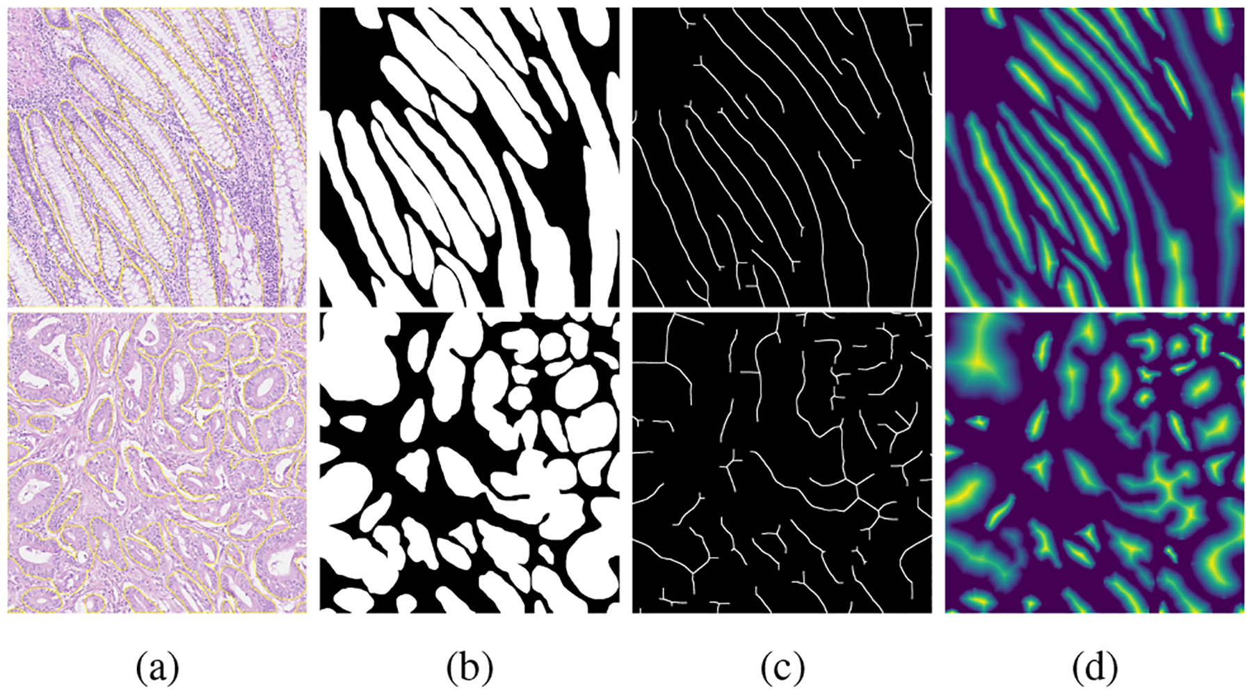
Examples of Medial axis (MA) transformation. a) A histopathology image patch with labeled (yellow contours) clustered glands; b) the binary annotation of gland regions; c) the topological skeletons of glands, noted that skeletons are morphological dilated to be visible; and d) the MA distance map.

Examples of the MA distance map is shown in Figure. 5(d). As shown in Figure. 5(a), it is challenging to separate the clustered glands; however, in Figure. 5(c) and (d), the skeleton and distance map emphasize the geometrical and topological properties of each gland, and clearly separate all clustered glands. Eq.(3) and the MA transformation are applied to generate the ground truth for the MA distance map. To ensure that the proposed gland segmentation network preserves gland topology, we design the second decoder branch to predict the MA distance map. The loss function L_MA is defined by

$$L_{MA}=\frac{1}{m}\sum _{j=1}^m{\left(MA\left(p_j\right)-\widehat{MA}\left(p_j\right)\right)}^2$$ (4)

where $\widehat{MA}$ denotes the predicted distance map, and m is the number of image pixels.

Marker loss.

The Watershed algorithm is commonly applied as a postprocessing step to produce the fine segmentation, especially separating the clustered objects. The watershed markers represent the number and locations of objects, and are critical for accurate segmentation. More markers lead to over-segmentation, and fewer markers produce under-segmented results. We introduced the marker loss to separate clustered glands and prevent over-segmentation. The marker loss is defined as the Dice loss between predicted marker map $(\widehat{MC})$ and the true marker map (MC)

$$L_{MC}=\mathit{\text{Dice}}(MC,\widehat{MC})$$ (5)

The predicted marker map is generated by thresholding the outputs from the medial axis distance map.

4. Experimental Results

4.1. Datasets and Evaluation Metrics

Datasets.

The Colorectal adenocarcinoma gland (CRAG) dataset [12] and the Gland Segmentation challenge (GlaS) dataset [29] are used in this work. CRAG has 213 HE-stained histopathology images from 38 WSI images. The scanned image size is 1512 × 1516 pixels with the corresponding instance-level ground truth. The training set has 173 images and the test set has 40 images with different cancer grades. The GlaS dataset has 165 H&E-stained histopathology images extracted from 16 WSI images. The image size mostly is 775 × 522 pixels. The training set has 85 images (37 benign and 48 malignant). The test set is split into two sets: Test A (60 images) and Test B (20 images), because two test sets are releases in different stages in GlaS challenge. Both datasets are scanned with a 20× objective magnification. The CRAG dataset has more densely clustered glands.

Evaluation Metrics.

We use the F1-score, object-level Dice coefficient (Obj-D), and object-level Hausdorff distance (Obj-H). In the F1 score, a segmented gland is counted as a true positive if it has 50% overlap with the ground truth, and counted as a false positive (FP) if otherwise; and all missed glands in the ground truth are counted as false negatives. Refer to [29] for detailed descriptions of the Obj-D and Obj-H in Colon Histology Images Challenge Contest (GlaS) at MICCAI 2015.

4.2. Implementation Details

The TA-Net is trained and tested using a deep learning server with an NVIDIA Quadro RTX 8000 GPU, 512 GB memory, and two 2.4 GHz Intel Xeon 4210R CPUs.

The patch size of the GlaS dataset is 512 × 512 pixels, and the patch size of the CRAG dataset is 768 × 768 pixels. Different patch sizes are applied because 1) the two datasets have images with different sizes; and 2) larger patches improve the performance on segmenting white lumen regions inside the gland tissues. The larger patches could generate the whole white lumen region in the gland in one patch. The GlaS dataset generates 340 training patches and 320 test patches. The CRAG dataset generates 692 training patches and 160 test patches. The augmentation approaches, e.g., random flip, random rotation, Gaussian blur, and median blur, are utilized in the training stage. The segmentation results of image patches are merged to form images of the same size as the original images.

The training epoch is set as 200, and the initial learning rate for the Adam optimizer is set as 10–4 and is reduced to 10–5 after 100 epochs. The batch size is 4 for training the model.

The postprocessing applies the Watershed algorithm to produce the final output. We apply a threshold value to the outputs from the instance branch (INST) to generate the glands binary map, and utilize it as the Watershed filling region. The output from the MA distance branch are the local elevation of those glands. Further, thersholding the MA distance map to generate the Watershed markers. Morphology operations, e.g., fill the holes, remove the small objects are utilized to generate a fine glands regions and makers. In the end, the generated gland region, gland elevation and markers are input to Watershed algorithm for fine gland segmentation results.

4.3. Results and Discussion

In this section, we discuss the overall performance of our method, followed by the results using the contour map, and single-task/multitask networks. Finally, we discuss the performance of our network on different distance-metrics.

Overall performance.

We compare the proposed method with nine recently published approaches using the GlaS dataset and six approaches using the CRAG datasets. We implemented [1, 6, 5] by following the same strategies in the original papers and the rest of other results are cited from their original papers. The test performance of GlaS dataset is reported as the average performance on its test A and test B sets. We employed F1-score, object-level Dice coefficient (Obj-D), and object-level Hausdroff (Obj-H) distance to measure the overall performance.

Table 1 shows the test performance of different approaches on two public datasets. The proposed TA-Net outperforms all other methods on CRAG datasets in terms of the F1 score, Obj-D; and achieved the best results in Obj-D, Obj-H and the second-best results in F1-score on GlaS datasets. The GlaS dataset has a small number of densely clustered gland regions; therefore, comparing with the second-highest result (Yan et al. [8]), TA-Net is only slightly better, e.g. 4.3% improvement of the Obj-H. The CRAG dataset has more densely clustered glands, and our method improves the Obj-H significantly (19.3%). Figure. 6(d) demonstrates that TA-Net separates densely clustered glands accurately.

Table 1.

Overall segmentation performance on GlaS and CRAG datasets

Datasets	Methods	Year	F1(%)↑	Obj-D(%)↑	Obj-H↓
GlaS	SegNet[1]	2016	83.1	84.9	76.6
	DCAN[5]	2016	81.4	83.9	102.9
	DeepLab[6]	2017	83.7	84.5	80.5
	MILD-Net[12]	2019	87.9	87.5	73.7
	Micro-Net[23]	2019	86.5	87.6	70.4
	FullNet[22]	2019	88.9	88.5	63.0
	DSE[32]	2019	89.4	89.9	55.9
	MSFCN[8]	2020	89.3	89.9	53.1
	Yan et al.[34]	2020	90.7	89.3	58.7
	TA-Net	2021	90.5	90.2	50.8
CRAG	SegNet[1]	2016	77.4	85.3	134.7
	DCAN[5]	2016	73.6	79.4	218.8
	DeepLab[6]	2017	64.8	74.5	281.4
	MILD-Net[12]	2019	82.5	87.5	160.1
	DSE[32]	2019	83.5	88.9	120.1
	MSFCN[8]	2020	82.5	89.2	130.4
	TA-Net	2021	84.2	89.3	105.2

Figure 6.

Segmentation results of five image patches (top three from CRAG, bottom two from GlaS). Different colors represent different glands. Yellow dash region highlighted the clustered gland regions.

MA distance map vs. contour map.

We compared the proposed TA-Net with a multitask network (Ours-CNT) which has the same architecture as TA-Net but outputs the gland instance map and the gland contour map. The only difference between the two networks is that TA-Net uses the MA distance map, while Ours-CNT uses the gland contour map as the ground truth of the second decoder. As shown in Table.2, TA-Net comparing to the Ours-CNT, Obj-H has been improved by 5.7% and 35% on the GlaS and CRAG datasets, respectively. The results demonstrate that the network using the MA distance map generates more accurate gland contours than the contour map based network, especially on the CRAG dataset. Fig. 6 demonstrates that contour map-based strategy fails to separate many clustered glands (in dashed rectangles).

Table 2.

Ablation study on multitask learning and decoders

Datasets	Methods	F1(%)↑	Obj-D(%)↑	Obj-H↓
GlaS	Ours-INST	86.4	88.3	65.4
	Ours-MA	80.2	84.2	105.8
	Ours-CNT	89.1	88.2	54.4
	TA-Net	90.5	90.2	50.8
CRAG	Ours-INST	78.9	86.1	125.6
	Ours-MA	74.8	80.3	200.8
	Ours-CNT	81.3	85.8	164.5
	TA-Net	84.2	89.3	105.2

Multitask network vs. Singletask network.

In addition, we comparing the proposed multitask learning network with the single task learning network, which outputs the binary instance branch only (Ours-INST), and MA distance branch only (Ours-MA). In experiment of the Ours-INST, the Watershed algorithm is applied in the postprocessing for separating the clustered glands. In experiment of MA distance branch, we outputs the MA distance branch only. In the post-processing, we utilized the thresholding to produce a binary gland region map, and gland markers. Then, the Watershed is used to produce the final segmentation. From the Table. 2, we noted that the designed multitask learning network outperform one task networks (Ours-INST, Ours-MA). Integrating both gland instance and MA distance map will produce a reliable performance in gland segmentation.

W/ or w/o the marker loss.

The proposed TA-Net is compared with the same network without the marker loss (Ours-WoM). Table. 3. shows the results on two public datasets. From the quantitative results, we noted that the marker loss only improves the overall performance slightly on both two datasets. But we observed that the marker loss alleviates the over-segmentation and under-segmentation problems in clustered glands and deformed glands in many qualitative cases (Fig. 7).

Table 3.

Ablation study on marker loss

Datasets	Methods	F1(%)↑	Obj-D(%)↑	Obj-H↓
GlaS	Ours-WoM	90.2	89.8	54.4
	TA-Net	90.5	90.2	50.8
CRAG	Ours-WoM	83.7	89.1	108.6
	TA-Net	84.2	89.3	105.2

Figure 7.

Examples of the effectiveness of the marker loss.

Comparison on various distance map.

Deep Watershed-based regression algorithms provide the successful demonstration to separate the occluded objects and overlapped objects [2]. Most related method to ours is by Naylor et al. [18], which proposed a chessboard distance-based deep regression network for nuclei segmentation. First, comparing to their U-Net shape architecture, we employed the multitask learning-based Densely connected SegNet. We achieved promising performance in segmenting the gland foreground from the background. Second, the Medial Axis distance map preserve the topological property of the objects, which maintain the gland structure information during the training stage. Third, the marker loss will control the over-segmentation and under-segmentation issue for accurate marker detection.

To demonstrate the effectiveness of MA distance transform with other distance-based metrics, we set up an experiment using our network test with different distance metrics, includes the Euclidean distance, Chessboard distance, Medial axis (MA) distance. To conduct a fair comparison, marker loss will not apply in this study, and we replace the MA distance metrics to other distance metrics. Similar to our post-processing approach, the predicted gland foreground segmentation and the predicted distance map are utilized to produce the final fine segmentation. From the results in Table. 4., we noted that our methods outperform the other two distance metrics. It gives the fact that medial axis distance metrics achieved the best performance comparing to use Euclidean and chessboard distance metrics.

Table 4.

Ablation study on different distance metrics on CRAG dataset.

Datasets	Metrics	F1(%)↑	Obj-D(%)↑	Obj-H↓
GlaS	Euclidean	82.4	78.7	65.4
	Chessboard	86.4	83.4	71.2
	MA	90.2	89.8	54.4
CRAG	Euclidean	76.5	81.2	257.5
	Chessboard	80.8	85.9	178.9
	MA	83.7	89.1	108.6

5. Conclusion

In this paper, we propose a topology-aware network (TA-Net) to address the challenge of partitioning densely clustered glands in histopathology images. Firstly, the proposed multitask learning architecture integrates both instance segmentation and gland topology learning and learns their shared representation. Experimental results show that TA-Net outperforms the state-of-art multitask architectures, e.g., DCAN, and single-task architectures. Secondly, we propose a topology loss using Medial Axis distance map and gland makers. The loss penalizes the topology changes between the segmented glands and actual glands. The extensive experimental results on two public datasets demonstrate that the proposed TA-Net achieves state-of-the-art performance for densely clustered gland segmentation. In the future, we will extend the proposed approach to other challenging tasks, such as nuclei segmentation and semantic image segmentation.

References

- [1].Badrinarayanan Vijay, Kendall Alex, and Cipolla Roberto. Segnet: A deep convolutional encoder-decoder architecture for image segmentation. IEEE transactions on pattern analysis and machine intelligence, 39(12):2481–2495, 2017. [DOI] [PubMed] [Google Scholar]
- [2].Bai Min and Urtasun Raquel. Deep watershed transform for instance segmentation. In Proceedings of the IEEE Conference on Computer Vision and Pattern Recognition, pages 5221–5229, 2017. [Google Scholar]
- [3].Bloom HJG and Richardson WW. Histological grading and prognosis in breast cancer: a study of 1409 cases of which 359 have been followed for 15 years. British journal of cancer, 11(3):359, 1957. [DOI] [PMC free article] [PubMed] [Google Scholar]
- [4].Blum Harry et al. A transformation for extracting new descriptors of shape, volume 43. MIT press; Cambridge, MA, 1967. [Google Scholar]
- [5].Chen Hao, Qi Xiaojuan, Yu Lequan, and Heng Pheng-Ann. Dcan: deep contour-aware networks for accurate gland segmentation. In Proceedings of the IEEE conference on Computer Vision and Pattern Recognition, pages 2487–2496, 2016. [Google Scholar]
- [6].Chen Liang-Chieh, Papandreou George, Kokkinos Iasonas, Murphy Kevin, and Yuille Alan L. Deeplab: Semantic image segmentation with deep convolutional nets, atrous convolution, and fully connected crfs. IEEE transactions on pattern analysis and machine intelligence, 40(4):834–848, 2017. [DOI] [PubMed] [Google Scholar]
- [7].Clough James, Byrne Nicholas, Oksuz Ilkay, Zimmer Veronika A, Schnabel Julia A, and King Andrew. A topological loss function for deep-learning based image segmentation using persistent homology. IEEE Transactions on Pattern Analysis and Machine Intelligence, 2020. [DOI] [PMC free article] [PubMed] [Google Scholar]
- [8].Ding Huijun, Pan Zhanpeng, Cen Qian, Li Yang, and Chen Shifeng. Multi-scale fully convolutional network for gland segmentation using three-class classification. Neurocomputing, 380:150–161, 2020. [Google Scholar]
- [9].Egger Jan. Pcg-cut: graph driven segmentation of the prostate central gland. PloS one, 8(10):e76645, 2013. [DOI] [PMC free article] [PubMed] [Google Scholar]
- [10].Estrada Rolando, Tomasi Carlo, Schmidler Scott C, and Farsiu Sina. Tree topology estimation. IEEE transactions on pattern analysis and machine intelligence, 37(8):1688–1701, 2014. [DOI] [PMC free article] [PubMed] [Google Scholar]
- [11].Fleming Matthew, Ravula Sreelakshmi, Tatishchev Sergei F, and Wang Hanlin L. Colorectal carcinoma: Pathologic aspects. Journal of gastrointestinal oncology, 3(3):153, 2012. [DOI] [PMC free article] [PubMed] [Google Scholar]
- [12].Graham Simon, Chen Hao, Gamper Jevgenij, Dou Qi, Heng Pheng-Ann, Snead David, Tsang Yee Wah, and Rajpoot Nasir. Mild-net: Minimal information loss dilated network for gland instance segmentation in colon histology images. Medical image analysis, 52:199–211, 2019. [DOI] [PubMed] [Google Scholar]
- [13].Hu Xiaoling, Li Fuxin, Samaras Dimitris, and Chen Chao. Topology-preserving deep image segmentation. In Wallach H, Larochelle H, Beygelzimer A, d’Alché-Buc F, Fox E, and Garnett R, editors, Advances in Neural Information Processing Systems, volume 32. Curran Associates, Inc., 2019. [Google Scholar]
- [14].Huang Gao, Liu Zhuang, Van Der Maaten Laurens, and Weinberger Kilian Q. Densely connected convolutional networks. In Proceedings of the IEEE conference on computer vision and pattern recognition, pages 4700–4708, 2017. [Google Scholar]
- [15].Long Jonathan, Shelhamer Evan, and Darrell Trevor. Fully convolutional networks for semantic segmentation. In Proceedings of the IEEE conference on computer vision and pattern recognition, pages 3431–3440, 2015. [DOI] [PubMed] [Google Scholar]
- [16].Montironi Rodolfo, Mazzuccheli Roberta, Scarpelli Marina, Lopez-Beltran Antonio, Fellegara Giovanni, and Algaba Ferran. Gleason grading of prostate cancer in needle biopsies or radical prostatectomy specimens: contemporary approach, current clinical significance and sources of pathology discrepancies. BJU international, 95(8):1146–1152, 2005. [DOI] [PubMed] [Google Scholar]
- [17].Mosinska Agata, Marquez-Neila Pablo, Koziński Mateusz, and Fua Pascal. Beyond the pixel-wise loss for topology-aware delineation. In Proceedings of the IEEE conference on computer vision and pattern recognition, pages 3136–3145, 2018. [Google Scholar]
- [18].Naylor Peter, Marick Laé Fabien Reyal, and Walter Thomas. Segmentation of nuclei in histopathology images by deep regression of the distance map. IEEE transactions on medical imaging, 38(2):448–459, 2018. [DOI] [PubMed] [Google Scholar]
- [19].Nguyen Kien, Jain Anil K, and Allen Ronald L. Automated gland segmentation and classification for gleason grading of prostate tissue images. In 2010 20th International Conference on Pattern Recognition, pages 1497–1500. IEEE, 2010. [Google Scholar]
- [20].Noble Jack H and Dawant Benoit M. An atlas-navigated optimal medial axis and deformable model algorithm (nomad) for the segmentation of the optic nerves and chiasm in mr and ct images. Medical image analysis, 15(6):877–884, 2011. [DOI] [PMC free article] [PubMed] [Google Scholar]
- [21].Paul Angshuman and Mukherjee Dipti Prasad. Gland segmentation from histology images using informative morphological scale space. In 2016 IEEE International Conference on Image Processing (ICIP), pages 4121–4125. IEEE, 2016. [Google Scholar]
- [22].Qu Hui, Yan Zhennan, Riedlinger Gregory M, De Subhajyoti, and Metaxas Dimitris N. Improving nuclei/gland instance segmentation in histopathology images by full resolution neural network and spatial constrained loss. In International Conference on Medical Image Computing and Computer-Assisted Intervention, pages 378–386. Springer, 2019. [Google Scholar]
- [23].Ahmed Raza Shan E, Cheung Linda, Shaban Muhammad, Graham Simon, Epstein David, Pelengaris Stella, Khan Michael, and Rajpoot Nasir M. Micro-net: A unified model for segmentation of various objects in microscopy images. Medical image analysis, 52:160–173, 2019. [DOI] [PubMed] [Google Scholar]
- [24].Ronneberger Olaf, Fischer Philipp, and Brox Thomas. U-net: Convolutional networks for biomedical image segmentation. In International Conference on Medical image computing and computer-assisted intervention, pages 234–241. Springer, 2015. [Google Scholar]
- [25].Sebastian Thomas B, Klein Philip N, and Kimia Benjamin B. Recognition of shapes by editing shock graphs. In ICCV, volume 1, pages 755–762. Citeseer, 2001. [Google Scholar]
- [26].Shit Suprosanna, Paetzold Johannes C, Sekuboyina Anjany, Ezhov Ivan, Unger Alexander, Zhylka Andrey, Pluim Josien PW, Bauer Ulrich, and Menze Bjoern H. cldice-a novel topology-preserving loss function for tubular structure segmentation. In Proceedings of the IEEE/CVF Conference on Computer Vision and Pattern Recognition, pages 16560–16569, 2021. [Google Scholar]
- [27].Shotton Jamie, Girshick Ross, Fitzgibbon Andrew, Sharp Toby, Cook Mat, Finocchio Mark, Moore Richard, Kohli Pushmeet, Criminisi Antonio, Kipman Alex, et al. Efficient human pose estimation from single depth images. IEEE transactions on pattern analysis and machine intelligence, 35(12):2821–2840, 2012. [DOI] [PubMed] [Google Scholar]
- [28].Siddiqi Kaleem, Shokoufandeh Ali, Dickinson Sven J, and Zucker Steven W. Shock graphs and shape matching. International Journal of Computer Vision, 35(1):13–32, 1999. [Google Scholar]
- [29].Sirinukunwattana Korsuk, Pluim Josien PW, Chen Hao, Qi Xiaojuan, Heng Pheng-Ann, Guo Yun Bo, Wang Li Yang, Matuszewski Bogdan J, Bruni Elia, Sanchez Urko, et al. Gland segmentation in colon histology images: The glas challenge contest. Medical image analysis, 35:489–502, 2017. [DOI] [PubMed] [Google Scholar]
- [30].Tosun Akif Burak and Gunduz-Demir Cigdem. Graph run-length matrices for histopathological image segmentation. IEEE Transactions on Medical Imaging, 30(3):721–732, 2010. [DOI] [PubMed] [Google Scholar]
- [31].Tsogkas Stavros and Dickinson Sven. Amat: Medial axis transform for natural images. In Proceedings of the IEEE International Conference on Computer Vision, pages 2708–2717, 2017. [Google Scholar]
- [32].Xie Yutong, Lu Hao, Zhang Jianpeng, Shen Chunhua, and Xia Yong. Deep segmentation-emendation model for gland instance segmentation. In International Conference on Medical Image Computing and Computer-Assisted Intervention, pages 469–477. Springer, 2019. [Google Scholar]
- [33].Xu Yan, Li Yang, Wang Yipei, Liu Mingyuan, Fan Yubo, Lai Maode, Eric I, and Chang Chao. Gland instance segmentation using deep multichannel neural networks. IEEE Transactions on Biomedical Engineering, 64(12):2901–2912, 2017. [DOI] [PubMed] [Google Scholar]
- [34].Yan Zengqiang, Yang Xin, and Cheng Kwang-Ting. Enabling a single deep learning model for accurate gland instance segmentation: A shape-aware adversarial learning framework. IEEE transactions on medical imaging, 39(6):2176–2189, 2020. [DOI] [PubMed] [Google Scholar]