

Abstract
Traditional pulse-echo ultrasound imaging heavily relies on the discernment of signals based on their relative magnitudes but is limited in its ability to mitigate sources of image degradation, the most prevalent of which is acoustic clutter. Advances in computing power and data storage have made it possible for echo data to be alternatively analyzed through the lens of spatial coherence, a measure of the similarity of these signals received across an array. Spatial coherence is not currently explicitly calculated on diagnostic ultrasound scanners but a large number of studies indicate that it can be employed to describe image quality, to adaptively select system parameters and to improve imaging and target detection. With the additional insights provided by spatial coherence, it is poised to play a significant role in the future of medical ultrasound. This review details the theory of spatial coherence in pulse-echo ultrasound and key advances made over the last few decades since its introduction in the 1980s.
Keywords: Spatial coherence, Beamforming, Clutter reduction, Image quality characterization, Tissue characterization
INTRODUCTION
Pulse-echo ultrasound imaging has used delay and sum (DAS) beamforming to create images for several decades. A computationally lightweight process, DAS beamforming involves only three steps for image formation: (i) time-delaying individual array element signals based on the array geometry, (ii) their summing across the aperture to create a scan line and (iii) envelope detection to extract the echo magnitude from the amplitude-modulated ultrasound signal. These steps are repeated over multiple transmit events and delay configurations to form an image over the desired field of view. Accordingly, metrics for image quality assessment and tissue characterization have been developed that relate to signal amplitude and its distribution over a spatial extent (Patterson and Foster 1983; Smith et al. 1983; Smith and Wagner 1984; Hall et al. 1993). However, imaging and evaluation based on signal amplitude alone are complicated by the presence of acoustic clutter, one of the main hindrances to clinical DAS imaging. Clutter, which often manifests as a temporally stable haze resembling speckle, results from heterogeneities in tissue that introduce phenomena such as phase aberration, off-axis scattering and reverberation (O’Donnell and Flax 1988; Freiburger et al. 1992; Hinkelman et al. 1994; Lediju et al. 2008; Pinton et al. 2011; Dahl and Sheth 2014; Byram et al. 2015; Fatemi et al. 2019). The effects of clutter are exacerbated in patients with large body habitus, resulting in images of poor quality and clinical misdiagnoses (Lencioni et al. 2002; Uppot et al. 2006; Uppot 2007; Khoury et al. 2009; Dahl et al. 2017). Though there have been several major advances in clutter suppression over the last few decades, clutter remains the dominant source of image degradation in medical ultrasound, and efforts toward its mitigation remain at the forefront of ultrasound research.
Because DAS beamforming leverages only one property of array data, the signal magnitude, it remains limited in challenging clinical settings. However, exponential improvements in data storage and computing power have enabled other novel insights into the properties of array data. One such property is spatial coherence, which is reflective of signal similarity rather than signal amplitude. Though the history of coherence in optics is over two centuries long, its introduction to pulse-echo ultrasound has been relatively recent. Early observations in the correlation length of coherent ultrasonic speckle were first documented by Wagner et al. (1988), followed shortly by the translation of key principles in statistical optics to ultrasound in 1991 by Mallart and Fink (1991). This has since spurred three decades of research into the use of coherence for better discerning ultrasound echo signals. Early work in coherence in ultrasound largely focused on characterizing signal quality (Mallart and Fink 1994b; Hollman et al. 1999; Bamber et al. 2002; Li and Li 2003), but efforts to translate coherence properties to image formation quickly followed. By the late 2000s and early 2010s, spatial coherence had become a major area of research in medical ultrasound that continues today with new methods to form images (Synnevag et al. 2007; Camacho et al. 2009; Lambert et al. 2020a; Long et al. 2020b; Ozgun et al. 2020) and evaluate image quality (Lediju et al. 2011; Matrone and Ramalli 2018; Long et al. 2020a). Recent work in coherence also explores its ability to characterize tissue, serving as a biomarker to aid clinical diagnoses (Imbault et al. 2017; Papadacci et al. 2017; Offerdahl et al. 2020; Wiacek et al. 2020b).
This review is outlined as follows. First, the origins of spatial coherence theory in optics and its translation to pulse-echo ultrasound are detailed. Next, early strategies to identify and quantify coherence are reviewed in the context of evaluating focusing errors, followed by a review of parallel efforts to characterize the effects of channel noise on measured coherence. Then, key efforts in developing coherence-based beamformers and biomarkers are described. Lastly, challenges to and opportunities in the future of coherence in medical ultrasound are discussed. Approval of protocols for human and animal studies by an institutional review board or institutional animal care and use committee was part of the inclusion criteria for referenced work.
PRINCIPLES OF SPATIAL COHERENCE
Origins
The concept of spatial coherence originates from early observations in the interference of light. The patterns observed in Thomas Young’s double-slit experiment revealed that because phase is a wave property, there exist bright and dark “fringes,” corresponding to regions of constructive and destructive interference, respectively (Young 1804). The difference in fringe brightness, V, between constructive and destructive points was determined by Albert Michelson, who found it was a function of the distance between the slits, the distance between the source and the objective and the wavelength in the monochromatic case (Michelson 1890):
| (1) |
Here I1 and I2 are the intensities measured in a bright and dark fringe, respectively, λ is the wavelength, β is the ratio between the slit distance and the source-objective distance and a is the width of the slit. This calculated fringe brightness difference can be considered a preliminary measurement of the coherence of light, where large differences, that is, V → 1, indicate high coherence, and small differences, that is, V → 0, indicate low coherence.
The translation of this concept to incoherent sources using statistical optics was performed by the physicists Pieter Hendrik van Cittert (1934) and Frits Zernike (1938). They describe the mathematical framework by which the mutual intensity, that is, spatial coherence, may be predicted between two arbitrary observation points in space for a collection of independent radiators, which act as an incoherent source (Goodman 2015).
Theory in pulse-echo ultrasound
The concept of coherence in ultrasound originated with the characterization of speckle patterns observed in B-scans (Burckhardt 1978; Wagner et al. 1983). Understanding that speckle originates from a coherent wave, early work defined the first- and second-order statistics of ultrasonic speckle. The latter describes the correlation length of speckle, that is, correlations of different regions of speckle, and was found by Wagner et al. (1988) to be dependent on the aperture size and the translation distance between regions or over the aperture, paving the way for descriptions of signal similarity over spatial extents.
Later, Mallart and Fink (1991) extended the van Cittert–Zernike (VCZ) theorem to pulse-echo ultrasound, where the behavior of the incoherent source is dependent on the irradiation of the isochronous volume. This irradiation is time varying, that is, depth dependent, because of the diffraction effects over the course of propagation. Therefore, the VCZ theorem in pulse-echo ultrasound is not easily collapsible to a single, stationary incoherent source as is sometimes the case in traditional optics. There exist several derivations and adaptations of the VCZ theorem in ultrasound, including consideration of various sources of acoustic clutter and focusing errors (Mallart and Fink 1991, 1994; Liu and Waag 1995; Walker and Trahey 1997; Pinton et al. 2014), but a brief derivation of the theorem for the simple case of a focused, monochromatic transmission is as follows.
Spatial coherence may be defined as the statistical autocorrelation of the field between two points and . Given that the source is incoherent, the pressure at these spatial locations may be described as random processes, . The spatial coherence is thus described as
| (2) |
where ⟨·⟩is the ensemble average and * indicates the complex conjugate.
The backscattered pressure at an arbitrary point in space, , from a single scatterer located at may be calculated as
| (3) |
| (4) |
where f is the frequency, c is the speed of sound and and are the scattering function and frequency domain impulse response of the transmit aperture at , respectively. Note the frequency dependence of the two latter defined terms, a consequence of assumed Rayleigh scattering properties. A description of all relevant variables is found in Table 1.
Table 1.
Description of variables
| Variable | Description |
|---|---|
|
| |
| ψ | Pressure |
| f | Frequency |
| c | Speed of sound |
| Spatial location | |
| Scattering function | |
| Frequency domain impulse response | |
| k | Wavenumber |
| Spatial coherence between two points | |
| z | Depth or axial distance |
| x | Azimuth or transverse distance |
| Aperture function | |
| η | Root mean square time delay error |
| n | Time or axial sample |
| s(t) | Continuous signal at time t |
| s[n] | Discrete signal at sample n |
| M | Array elements in active aperture |
| m | Lag or element separation |
| R[m] | Spatial coherence at lag m |
The combined pressure field over a volume of scatterers is obtained by integrating over a volume of interest
| (5) |
where k is the wavenumber, equivalent to 2πf/c.
Returning to eqn (2), we can substitute the expression inside the ensemble average with this definition for the individual pressure fields, and simplify to integrate over a single volume after isolating the random variable, χ0(f)
| (6) |
| (7) |
The Fresnel approximation may be applied if the depth of observation, z, is large compared with the transverse distance between and , as is typically the case in ultrasound. Using and z to indicate the transverse and axial location of spatial point , and assuming zi = 0, ri in eqn (7) is well approximated by a Taylor series expansion,
| (8) |
This expression is then substituted into eqn (6), using only the first-order term, z, in non-phase terms. After simplification, eqn (6) reduces to:
| (9) |
In pulse-echo ultrasound, it is often useful to isolate signal at a particular depth, that is, pertaining to a single isochronous surface. In this case, z may be imposed as a constant, reducing the volume integration to a surface integration over an area within the isochronous volume:
| (10) |
To relate this formulation of the VCZ theorem to the transducer aperture function, we must first describe the frequency domain impulse response, , shown in eqn (5), in terms of the aperture function, :
| (11) |
| (12) |
where the integration is performed over the spatial extent of the aperture.
Early derivations set this extent as a 2-D space in the plane orthogonal to the axis of transmission (Fink and Cardoso 1984; Mallart and Fink 1991), that is, a planar aperture. In this case, when the Fresnel approximation in eqn (8) is applied, the impulse response is described as
| (13) |
Note that the subscript A is omitted from terms related to the aperture spatial extent for readability. The exponential terms inside the integral are not combined so as to highlight the integral serves as a 2-D Fourier transform of at spatial frequency . Rewriting this term as for readability, the power spectral density of the frequency domain impulse response is therefore
| (14) |
where and are position placeholder variables for the respective integrations over the aperture extent.
The expression is then combined with eqn (10) to produce
| (15) |
This may be further simplified to the form:
| (16) |
In this reduction, one can see that the spatial coherence has been simplified to the scaled autocorrelation of the complex aperture function, . Rewriting in a compact form,
| (17) |
where is the scaled autocorrelation of . This elegant result reveals that the spatial coherence is a function of the transverse separation between the points of inspection, and not the absolute location of each. The classic example of eqn (17) is the case of a linear array, whose aperture function is the rectangle function. Its autocorrelation is a triangle function, with base twice as wide as the length of the rectangle; this example is frequently used to calculate an analytical “ideal” spatial coherence function (Mallart and Fink 1991; Pinton et al. 2014; Long et al. 2018b).
Relationship to field profile
The relationship between the aperture function and the resulting spatial coherence function may also be described in terms of the Fourier transform relationships with the aperture function and field intensity profile. Figure 1 illustrates these relationships. Once again using the simple example of a 1-D array with flat apodization, the transmitted field pressure profile at the focus, a sinc, is the Fourier transform of the aperture function, per the Fraunhofer approximation. Thus, the field intensity profile, being the square of the pressure profile, is a sinc2 function. Because of the assumed spatial incoherence of the scatterers in the field, the field intensity profile can be applied as the source term in the VCZ theorem, which predicts the received spatial coherence as the Fourier transform of the intensity profile. The associated autocorrelation relationship (eqn (17)) is related to Norbert Wiener’s harmonic analysis for a deterministic function, whereby its autocorrelation is equal to the Fourier transform of its power spectral density (Wiener 1930).
Fig. 1.
Fourier transform (F.T.) relationships between the aperture function, field intensity profile and spatial coherence function. The aperture, shown at the top left, is a rectangle function in this example.
These relationships may also be tested with the thought experiment of an incoherent transmission. Intuitively, an incoherent transmission into incoherent media should yield a similarly incoherent received signal. Following the same Fourier transform relationships, the coherence function is the Dirac δ function, indicating no coherence outside of unity; the autocorrelation of a random function shows likewise. Note that incoherence introduced by phase or amplitude randomization is equivalent for a sample at a given depth or time (Bottenus and Trahey 2015). The implications of signal incoherence are discussed in later sections.
Though the aperture function is directly related to the transmit field profile, there exist other mechanisms by which the profile may be changed. Most prevalent in pulse-echo ultrasound are phase aberration and non-linear acoustics. The former arises from heterogeneities in the speed of sound of the medium that distort the transmit profile and redistribute energy in the beam from the main lobe to the side lobes (Steinberg 1976), resulting in a broader beam (Smith et al. 1988). Because of the scaling properties of the Fourier transform, a narrowing of the spatial coherence function would then be expected. Walker and Trahey (1997) derived a theoretical framework showing this phenomenon for a phase screen aberrator with known spatial autocorrelation full-width half maximum (FWHM) and root-mean-square (RMS) time delay error. The resulting decorrelation between the signals received at and for an aberrator with autocorrelation function is:
| (18) |
where f is the frequency and η is the RMS time delay error. On the basis of this model, the consequence of a phase screen aberrator is a Gaussian weighting of the intrinsic target coherence function, the magnitude and shape of which are dependent on the RMS error and autocorrelation FWHM, respectively. Though the derivation of VCZ theorem is frequency independent outside of the target scattering function, the effect of aberration is frequency dependent. As the frequency increases, fixed time delay errors become a greater fraction of the wavelength, leading to magnified phase errors.
Non-linear acoustics, often discussed in conjunction with tissue harmonic imaging (THI), introduce harmonic frequencies converted from energy at fundamental frequencies to the received signal as a result of wave propagation (Adler and Hiedemann 1962). The degree of non-linear signal transformation is related to the acoustic pressure and frequency, the density and non-linearity of the medium and the distance of propagation. As a result, the main lobe of the harmonic beam is wider than that of the beam created with a transmission at the second harmonic frequency, though with reduced sidelobes (Lencioni et al. 2002). Fedewa et al. (2003) reported that this beam broadening behavior acts like an effective apodization, resulting in roughly Gaussian decorrelation profiles in the spatial coherence function, similar in shape to those predicted by aberrators in eqn (18).
Shifting apertures, reciprocity and motion
The decorrelation as a function of spatial separation between point observers is mathematically predictive of that for spatially separated apertures, where the apertures substitute as observations. For shifting apertures, which are commonly used for spatial compounding (Trahey et al. 1986), the same general trend is observed: increases in spatial separation lead to decorrelation. For transmit aperture shift and receive aperture shift , the relationship between the aperture shift and frame correlation is defined as (Walker and Trahey 1997):
| (19) |
where A is the aperture function. Note the similarity between this formula and eqn (17): both measures of correlation are a function of the scaled autocorrelation of the aperture function, evaluated at different spatial separations. In fact, if one fixes either the transmit or receive aperture while allowing the other to shift, eqn (19) reduces to a form nearly identical to eqn (17). Bottenus and Ustüner (2015) indicate that this relationship, known as acoustic reciprocity, also holds for transmit and receive pairs of elements. By this principle, spatial coherence may be evaluated for pairs of transmit elements rather than pairs of receive elements. As is discussed in a later section, acoustic reciprocity has implications for synthetic aperture coherence beamforming.
Additional considerations for motion were detailed in the work of Hyun and Dahl (2020), who derived a general theory for the correlation of two echo signals with an arbitrary set of apertures and scatterer motion. A series of assumptions reveals that, in addition to the shifting apertures case described by eqn (19), the signal correlation may be predicted for bulk axial and transverse motion of scatterers. For example, axial scatterer motion contributes a phase shift; this principle is found in displacement estimators used in speckle tracking (Kasai and Namekawa 1985).
Calculation of coherence from echo data
In practice, spatial coherence may be computed with time-windowed correlations of signal received on any two array elements in the active aperture. In most applications of spatial coherence, the correlation is normalized to the signal intensity so as to provide a value between −1 and 1, though applications exploiting the non-normalized covariance exist. For the remainder of this review, calculations are presented only for 1-D arrays, unless otherwise noted. Note that for these calculations, the Fourier transform relationships illustrated in Figure 1 are valid only for a focused transmission near the focus; interrogation away from the focus introduces phase terms that reduce coherence. By replacing the generic transverse position with a coordinate in the azimuthal dimension (xi), the normalized correlation surface between any two spatially separated, time-varying signals in the active aperture, s(xi,t) and s(xj,t), is calculated as
| (20) |
where τ is the time window of correlation. This equation can be slightly modified to define a coherence matrix for discretely sampled signals, as is the case in medical ultrasound,
| (21) |
where ni and n2 are the sampling bounds of the correlation time window, typically set within the depth of field, and s is redefined as being discretely sampled in time and azimuthal position. There is a range of reported correlation window sizes, which include studies performed with single sample (Hyun et al. 2017), 1λ (Lediju et al. 2011) and 4λ (Papadacci et al. 2014) windows.
Lastly, this matrix may be flattened to a 1-D function by averaging the correlation between pairs of received signals with identical spatial separation, also known as lag:
| (22) |
Here M is the number of elements in the active aperture, and m is the element separation, that is, lag.
Hyun et al. (2017) derived an efficient method to calculate this function from complex in-phase and quadrature (I/Q) signals
| (23) |
where * again indicates the complex conjugate, and n is now the single time sample of interest. The overall process to arrive at a calculated coherence function is summarized in Figure 2. The process is shown in three stages. First, backscattered signals reflected from diffuse scattering media are received by an M-element array. Next, signals are time-delayed as is the case in DAS beamforming. Last, cross-correlations are calculated to form the coherence matrix and, most commonly, averaged to compute the coherence at a given lag, up to a maximum of M − 1 lags.
Fig. 2.
Three-stage process for calculation of the coherence function. First, signals are backscattered to an M-element array (red). Second, time delays are applied to received signals (blue). Third, correlation pairs are calculated for each lag of the coherence function (green).
APPLICATIONS TO IMAGING
The investigation of factors affecting image quality in medical ultrasound has been decades long. However, descriptions in terms of the spatial coherence are relatively new. A 1986 review by Kremkau and Taylor (1986) highlighted several artifacts in imaging, though the descriptions are largely qualitative, with no reference to each source’s contribution to losses in contemporary metrics of image quality (Patterson and Foster 1983; Smith et al. 1983; Smith and Wagner 1984; Hall et al. 1993). However, the concept of a stationary component to acoustic noise, also known as clutter, was well understood. Clutter degrades images by distorting contrast and obscuring boundaries and fine details, and remains a major limitation to the diagnostic power of medical ultrasound (Hendler et al. 2004; Irshad et al. 2012; Tsai et al. 2015; Simmons et al. 2017). Though clutter is exacerbated in subjects with large patient body habitus, because of multilayered, thick abdominal walls, it exists to some degree in all ultrasonic imaging because of the presence of off-axis energy in both the transmit and receive point-spread functions (Dahl et al. 2017; Bottenus et al. 2020). The primary sources of clutter in medical ultrasound are phase aberration, reverberation and bright off-axis scattering (Ledoux et al. 1997; Zwirn and Akselrod 2006; Lediju et al. 2008; Pinton et al. 2011; Byram et al. 2015; Shin and Huang 2017).
Spatial coherence offers alternative strategies to image quality characterization and beamforming by placing less importance on signal magnitude, which may be misleading in the presence of clutter, and more importance on signal similarity. The development of coherence-based metrics has greatly advanced the field’s understanding of clutter mechanisms and has provided new avenues to develop beamforming and signal processing methods. In this section, we review the broad categories of coherence metrics and beamforming strategies developed over the last few decades.
Focusing errors
Early strategies for clutter compensation gave specific attention to the effects of wavefront aberration on focusing quality, which led to extensive measurements of the range of distortions observed in human tissue (O’Donnell and Flax 1988; Sumino and Waag 1991; Freiburger et al. 1992; Mast et al. 1998). In a series of studies, Hinkelman et al. (1994, 1995,1998) evaluated the pulse distortion through various tissue models and found a wide range of arrival errors, profile correlation lengths and degrees of similarity to a reference waveform.
Mast et al. (1997) observed and characterized the distortions introduced in simulation by propagation through an in silico heterogeneous layer, an example of which is illustrated in Figure 3. The ballistic wavefront is exposed to aberrations and complex reverberation events that result in acoustic energy trailing the wavefront; reverberation is discussed in a later section. As the wavefront advances through the heterogeneous layer, its phase aberrations increase in spatial frequency and further add to degradations in the coherent energy sum received at the transducer face. Some of the early strategies for clutter compensation sought to correct time delay errors by improving the coherent sum on beamforming through temporally aligning received signals or, equivalently, increasing speckle brightness with iterative timing adjustments (Nock et al. 1989; Karaman et al. 1993; Krishnan et al. 1996, 1997; Napolitano et al. 2006).
Fig. 3.
Propagation through fat and septa in a computerized human abdominal wall. Frames are shown 3.8 apart in time μs, and the area is 22.9 × 14.4 mm. Light blue regions of the abdominal wall correspond to fat; dark blue regions correspond to connective tissue. Reprinted, with permission, from Mast et al. (1997).
One of the earliest measures of the degree of wavefront coherence was the coherence factor (CF), introduced by Hollman et al (1999). It is defined as the ratio of the square of the coherent sum across array elements to the square of the incoherent sum:
| (24) |
Here n is again the time sample of interest; an axial average may also be taken over a range of n.
The CF is a measure of the wavefront uniformity and, by extension, the energy present in the main lobe relative to the side lobes (Steinberg 1976). In environments with aberration, the coherent sum in the numerator is reduced relative to the incoherent sum, and the CF is also reduced. The CF later gave rise to a spectral domain description of this ratio, dubbed the generalized coherence factor (GCF), where the energy in low-frequency regions of the spatial spectrum is compared with the total energy in the spectrum (Li and Li 2003)
| (25) |
where S[k] is the discrete spectrum of the channel radio-frequency (RF) data, and K is the number of points in the spectrum.
This principle of measuring the coherent summation is mirrored in the derivation of the focusing criterion described by Mallart and Fink (1994a). The authors report the coherent intensity is simply a discrete integration of the spatial coherence function, weighted by the autocorrelation of the aperture function, RAA[m],
| (26) |
where the second equality may be made for rectangular apertures. Note that the summation on the left-hand side is over M channels, whereas the latter two summations are over M − 1 lag pairs.
The focusing criterion, which is also a ratio between the coherent and incoherent intensities, is defined in terms of the spatial coherence as:
| (27) |
where R[0] is the peak of the coherence function. Liu and Waag (1994) independently derived a similar criterion known as the waveform similarity factor. This focusing criterion was employed by Måsøy et al. (2005) in an iterative aberration correction scheme, where the phase screen is estimated to inform the transmit delays. This concept of iterative correction of the transmit, rather than relying on received echoes of a distorted transmit, bears similarity to the time reversal mirror proposed by Fink (1992).
The relationship between spatial coherence and coherent intensity in the numerator of the focusing criterion is nearly identical to that between the former and beamformer gain, G, described by Bamber et al. (2002). Beamformer gain describes the ratio of the beamformed signal power to the total power of all signals in the active aperture as well as the ratio of the beamformed SNR (SNRbf) to the channel SNR (SNRc). For a rectangular aperture with flat weighting, it is calculated as:
| (28) |
The parallel between beamformer gain and coherent intensity highlights a key concept in understanding the spatial coherence function: encoded within the aperture domain is an expectation of the noise reduction and, by extension, SNR improvement in DAS beamforming. The next useful measurement then is the relative level of noise in each of the channel signals.
Channel noise
The other component of signal quality related to coherent intensity and beamforming gain is the level of noise in the echoes received at individual channels. This channel noise often arises from additive time domain sources, such as multiple reverberations, off-axis scattering and thermal noise (Ledoux et al. 1997; Zwirn and Akselrod 2006; Lediju et al. 2008; Pinton et al. 2011; Dahl et al. 2012; Dahl and Sheth 2014; Byram et al. 2015; Shin and Huang 2017). Multiple reverberations and off-axis scattering arise from reflections of the ballistic wave in tissue layers or specular structures, such as bone. These reflections result in signal overlaying that of the underlying tissue and may be incoherent or partially coherent, dependent on the reflection geometry. Recalling Figure 3, signal resulting from reverberation can be seen trailing the ballistic wavefront as it propagates through the abdominal layers (Mast et al. 1997).
Thermal noise refers to the relative amplification of electronic noise in low-signal environments, often in cases of high thermoviscous attenuation, tissue harmonic imaging and imaging at depth (Lencioni et al. 2002). It is closely related to the electrical and mechanical properties of the transducer (Goldberg and Smith 1995; Oakley 1997). Figure 4, from the work of Flint et al. (2021), illustrates the losses in image quality with increases in thermal noise. Low acoustic output corresponds to low mechanical index (MI), a measurement of acoustic exposure related to the peak negative pressure and frequency, and at these low outputs, image quality is poor.
Fig. 4.
Transverse fetal abdomen acquisition at four different acoustic output levels, labeled with corresponding mechanical indices. Images are shown over a 70-dB dynamic range, and axes are in centimeters. Reprinted, with permission, from Flint et al. (2021). MI = mechanical index.
In the case of spatially incoherent channel noise, as is generally the case in diffuse reverberation and thermal noise, the aperture domain representation of the noise is commonly the Dirac 8 function (Pinton et al. 2014). When superimposed on the inherent target coherence function, this results in a jump discontinuity at the first lag. An example coherence function in the presence of incoherent noise is compared with the ideal case and that in the presence of partially coherent noise, such as aberration, in Figure 5. In the spatially incoherent model of noise, because the level of incoherent noise is encoded in the lag one value, Long et al. (2018b) determined that only the first lag is needed to assess this noise type, unlike that for partially coherent sources. The resulting metric, lag one coherence (LOC), has since found use in adaptive imaging strategies seeking to minimize thermal noise while limiting acoustic exposure; Figure 4 illustrates that, for this particular patient, minimal gains in image quality are seen above mechanical index (MI) = 0.64, which is significantly below the maximum MI interrogated in the study (1.2) and the MI limits imposed by the U.S. Food and Drug Administration (Nyborg 2000; Flint et al. 2021). This study found a correlation between LOC and traditional image quality metrics, with both leveling off near the MI above which minimal gains in image quality are observed. LOC has also found use in adaptively selecting transmit frequencies to maximize target detectability by balancing the improved resolution afforded by higher frequencies and the increase in aberration-associated clutter and resulting decorrelation (Long et al. 2018a).
Fig. 5.
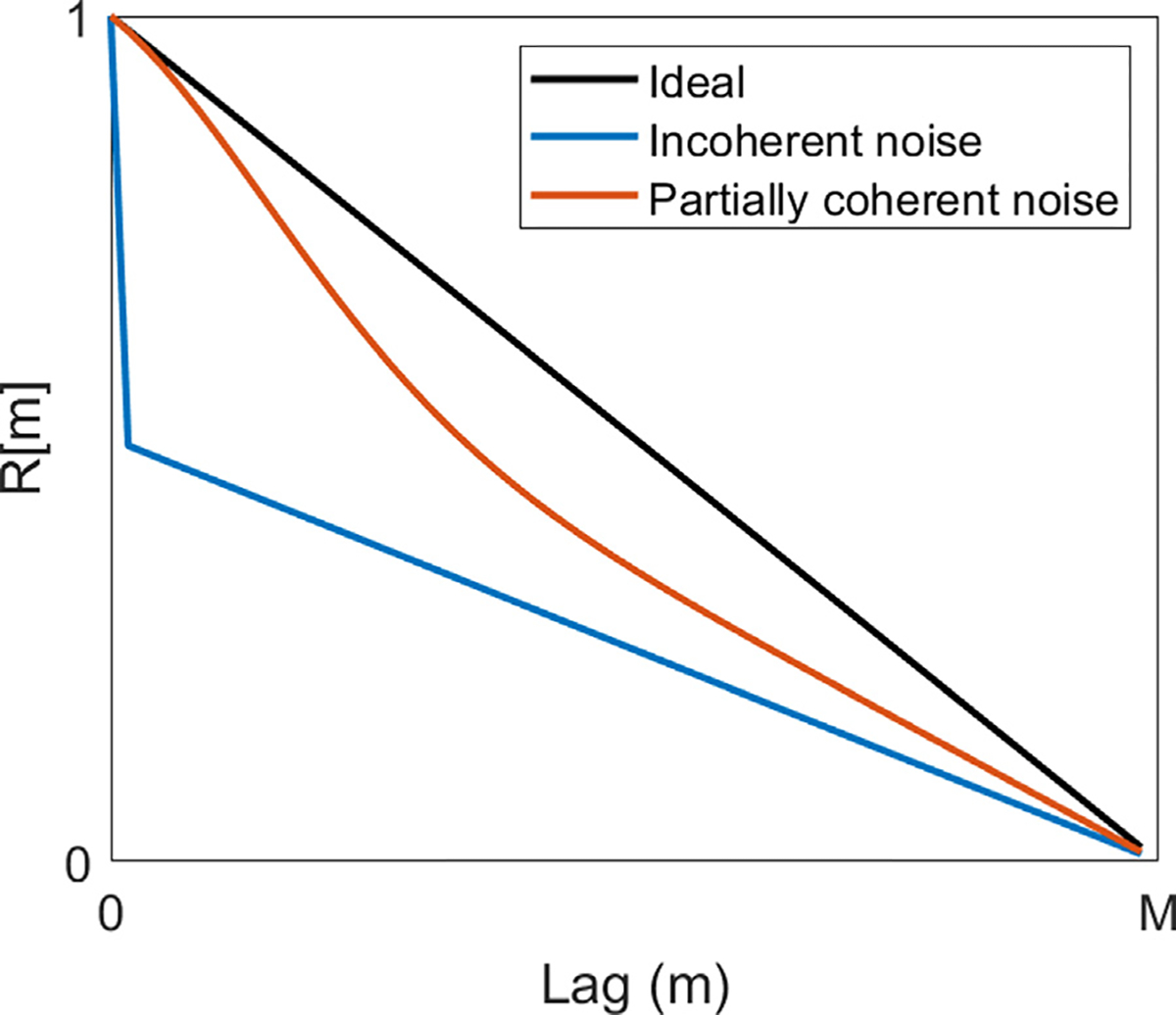
Illustration of the analytic spatial coherence function in the ideal, noise-free case (black) and in the presence of incoherent (blue) and partially coherent noise (red). Analytic calculation performed using the framework from Walker and Trahey (1997).
LOC is related to the SNRc as
| (29) |
where the approximation may be made for large, clinically relevant aperture element counts. LOC has been extended as an SNR-based, pixelwise compensation factor to correct the brightness in areas of low coherence, that is, high levels of incoherent clutter (Long et al. 2020b).
The SNRc estimated by LOC can also be combined with the maximum beamforming gain for the aperture, Gmax, to calculate the expected contrast of a target with known native contrast, C0:
| (30) |
This calculation may be extended to include decorrelation caused by phase aberration and other sources of partial decorrelation. By replacing the Gmax term with a lag one-corrected beamformer gain, Long et al. (2020a) found that contrast predictions may be extended to environments with incoherent noise and phase screen aberrators. Note that the metrics referenced in this subsection heavily rely on the assumption that additive channel noise is incoherent; efforts into characterizing partially coherent noise and its effects on beamforming are ongoing.
Short-lag spatial coherence beamforming
The measurements of coherent intensity, beamformer gain and channel noise have considerable overlap in that they are heavily dependent on coherence values in the early lags of the spatial coherence function. Because of this, one may interrogate only the short-lag region of the coherence function to capture the majority of decorrelation caused by clutter. This is the principle of short-lag spatial coherence (SLSC) beamforming, which is the most widely explored coherence beamformer in medical ultrasound.
Short-lag spatial coherence forms pixels based on a partial integration of the coherence function over the first N lags, where typical values of N are between 10% and 30% of the active aperture size, and may be parameterized as Q, a fraction of the active aperture size, M (Lediju et al. 2011):
| (31) |
Figure 6 illustrates the original results from the work of Lediju et al. (2011). In images of a human thyroid, SLSC beamforming outperforms conventional DAS beamforming and spatial compounding in CNR, and also has improved lateral resolution compared with the spatially compounded case for three values of Q. This series of images also illustrates the range of imaging texture made possible by tuning Q; as Q is increased, resolution improves at the expense of texture caused by the introduction of high-spatial-frequency information at higher lags in the spatial coherence function. A later work by Lediju Bell et al. (2015) confirmed this effect and also found that axial resolution was degraded with increasing kernel length used in the calculation (n1 to n2 in eqn (22)). Additionally, the contrast in SLSC images was found to be superior to that of conventional DAS beamforming. SLSC has been successfully extended to suppress clutter in a wide range of clinical applications, including cardiac, fetal and liver imaging, with measurable improvements in CNR (Dahl et al. 2011, 2012; Jakovljevic et al. 2013; Lediju Bell et al. 2013a; Long et al. 2018c). It has been used in contrast-enhanced ultrasonography (CEUS) to enhance molecular imaging in tumor microvasculature (Hyun et al. 2018), and in flow imaging to improve vessel detection (Li and Dahl 2015; Li et al. 2016; Ozgun et al. 2020).
Fig. 6.
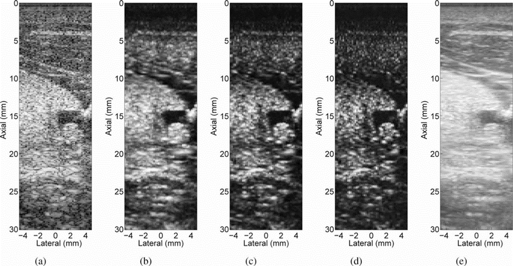
In vivo images of a cyst at a depth of 1.5 cm in a human thyroid: (a) B-mode, (c) short-lag spatial coherence at Q = 10.4%, (c) Q = 20.8%, (d) Q = 31.2% and (e) a spatially compounded image. All images are shown with a 50-dB dynamic range. Reprinted, with permission, from Lediju et al. (2011).
An example of a cardiac application is illustrated in Figure 7, from the work of Hyun et al. (2019). Using GPU-based coherence beamformers, Hyun et al. determined the feasibility of real-time SLSC imaging, with frame rates greater than 30 fps. In this pair of still images, bright clutter visible at the apex of the left ventricle in traditional tissue harmonic imaging is suppressed in the harmonic spatial coherence image.
Fig. 7.
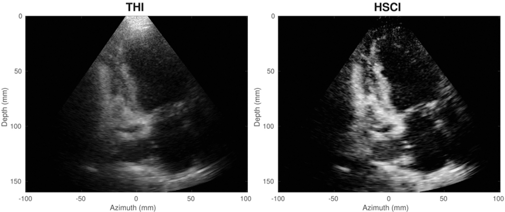
Tissue harmonic image (THI, left) and harmonic spatial coherence image (HSCI, right) of an apical two-chamber view for a cardiac patient. Reprinted, with permission, from Hyun et al. (2019).
Nair et al. (2018) proposed an improvement to SLSC, whereby the fixed integration limit in eqn (31) is relaxed to allow for adaptive beamforming on image subregions. By treating each coherence image as a noisy version of the intrinsic spatial coherence, a linear weighting scheme scaling with N may be applied to each image and summed to arrive at an M-weighted SLSC image. Alternatively, these weights may be determined via robust principal component analysis (RPCA), which searches for high-energy, low-dimension traces to extract an estimate of the contribution of each lag to the intrinsic coherence. This method, known as R-SLSC, has yielded considerable improvement in the diagnostic certainty of identifying fluid from solid masses in breast images, which would reduce the number of unnecessary biopsies (Wiacek et al. 2019, 2020b).
Short-lag spatial coherence has also been extended to advanced beamforming strategies to similar degrees of success. Synthetic aperture beamforming combines echo data from multiple transmissions with weak focusing to achieve retrospective dynamic transmit focusing and may be used to overcome the narrow depth-of-field often seen in coherence imaging as well as the loss in lateral resolution stemming from the loss of high spatial frequency information in the partial integration (Bottenus et al. 2013; Zhao et al. 2017). Additionally, SLSC has been employed with multiline transmissions to improve contrast in highly coherent structures (Matrone et al. 2021). SLSC may also be extended to matrix array beamforming, though additional considerations must be taken to redefine the short-lag region. Hyun et al. (2014) propose using theoretical correlation thresholds to define the aperture domain extent of integration. With these thresholds, improvements in detectability measures have been documented in vivo, even in 1.5-D and 1.75-D arrays (Jakovljevic et al. 2014; Morgan et al. 2019a).
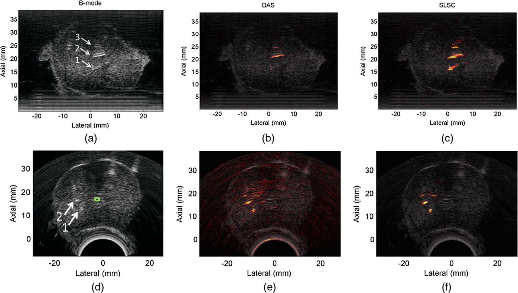
The principles of SLSC beamforming have been adapted to perform similar measurements on plane wave pulse-echo sequences. This translation rests on the principles of acoustic reciprocity, whereby the coherence evaluated at spatially separated transmit locations is equivalent to the coherence evaluated at identically separated receive locations for the same pulse-echo sequence (Bottenus and Ustüner 2015). In other words, the coherence measured between frames acquired at different transmit plane wave angles provides information similar to that measured between different receive array elements. This method, dubbed short-lag angular coherence (SLAC), obeys the VCZ theorem when the analytic expressions are modified to estimate loss in coherence as a function of the transmit angle, rather than spatial distance (Li and Dahl 2017). Figure 8 illustrates the work of Jakovljevic et al. (2021) in translating SLAC beamforming to power Doppler (PD) imaging, whereby SLAC-beamformed frames are used in place of B-mode frames for power estimation. In this image of a neonatal brain cortex, SLAC PD improves the SNR and increases the visibility of small vasculature, marked with white arrows.
Fig. 8.
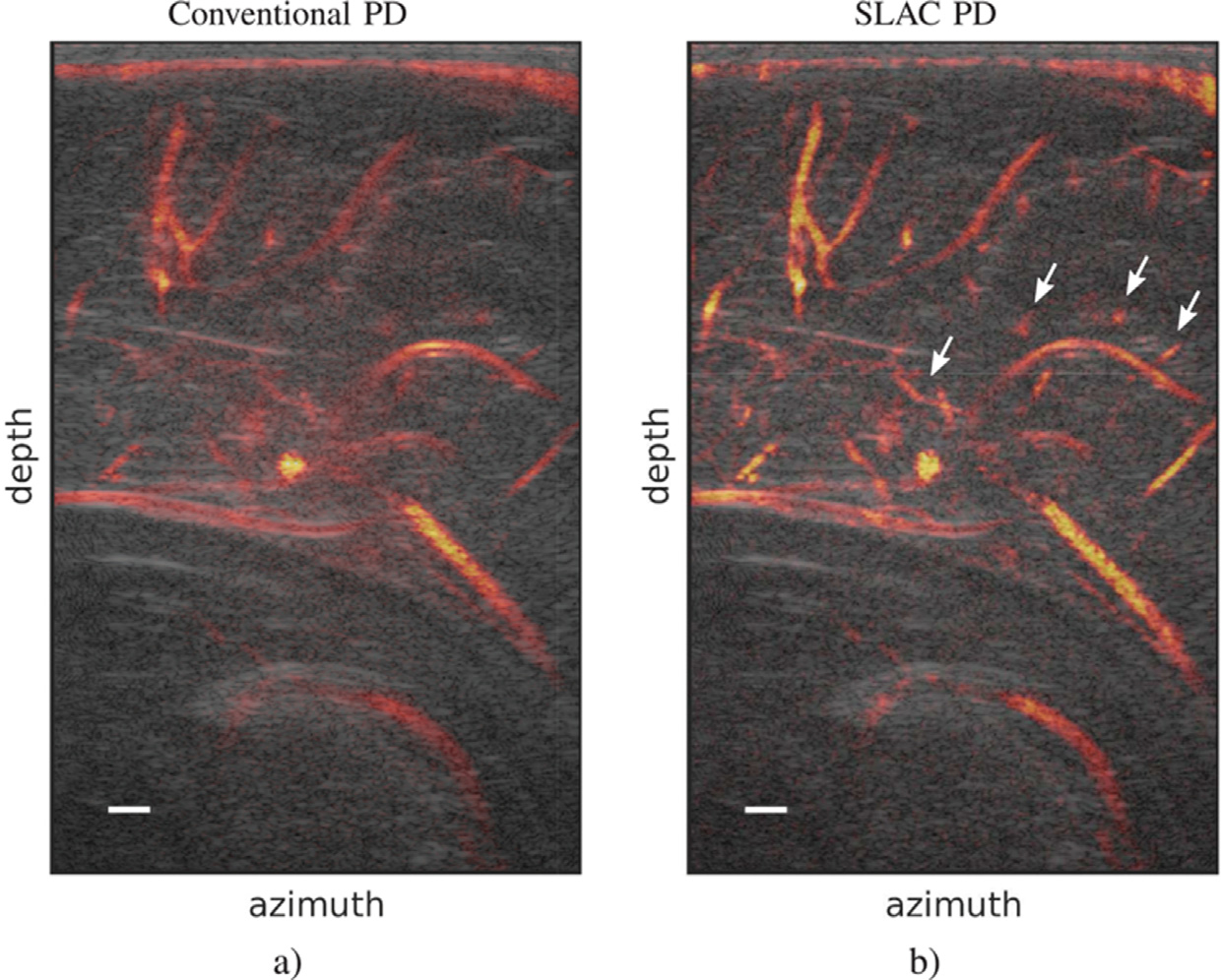
Power Doppler (PD) images revealing a sagittal view of a neonatal brain cortex for (a) conventional PD and (b) short-lag angular coherence (SLAC) PD. PD images are shown as an overlay to the B-mode. Arrows indicate small vasculature discernible in SLAC PD, but not in conventional PD. Reprinted, with permission, from Jakovljevic et al. (2021).
The integration of lags in the SLSC calculation (eqn [31]) may be truncated to the mid-lag region to arrive at mid-lag spatial coherence (MLSC), a strategy used to improve coherent target detection in diffuse scattering environments. Described by Tierney et al. (2019), MLSC is calculated from plane wave synthetic aperture data, focused on receive but not on transmit, and uses only the mid-lag region to differentiate coherent targets, such as kidney stones, from background tissue. When combined with incoherent compounding, which further suppresses tissue-based coherence, dramatic improvements in visualization are observed. MLSC has also been found to improve the detectability of gas bubbles for the purposes of mitigating gas embolism in intravascular oxygenation (Bottenus et al. 2021b).
Lastly, venturing beyond pulse-echo ultrasound, SLSC has found use in photo-acoustic beamforming, where the field acoustic intensity is generated with laser pulses and the photo-acoustic effect, rather than a transmitted acoustic pulse (Lediju Bell et al. 2013b; Pourebrahimi et al. 2013; Bell et al. 2014; Graham and Bell 2020; Gonzalez and Bell 2020). An example of SLSC-based photoacoustic imaging is provided in Figure 9. In a study by Bell et al. (2014) SLSC photo-acoustic imaging was used to improve visualization of brachytherapy seeds placed in an ex vivo dog prostate. In both linear and curvilinear arrays, the seeds are shown with higher SNR in the photo-acoustic cases, with the SLSC case further outperforming DAS photo-acoustic imaging. Photo-acoustic noise present near the lateral center in Figure 9e is suppressed in the SLSC case.
Fig. 9.
Brachytherapy seed visualization with B-mode (a, d), delay and sum (DAS) photo-acoustic imaging (b, e) and short-lag spatial coherence (SLSC) photo-acoustic imaging (c, f), for linear (a–c) and curvilinear (d–f) arrays. Photo-acoustic images are shown as an overlay to the B-mode. Arrows and numbers in the B-mode indicate the position of visible seeds, and the urethra is indicated with green. Reprinted, with permission, from Bell et al. (2014).
Other beamforming strategies
While pixel brightness is informed strictly by the measured coherence in SLSC, other beamforming strategies seek to combine coherence information with that afforded by signal amplitude. A variety of pixel-weighting schemes exist, including the previously discussed CF (Hollman et al. 1999; Li and Li 2003; Camacho et al. 2009; Nilsen and Holm 2010; Long et al. 2020b).
Camacho et al. (2009) introduced an extension of the CF that uses phase similarities to characterize the focusing quality. When applied as pixel weights, this new metric, the phase coherence factor (PCF), was found to decrease sidelobe energy and improve the resolution of point targets in simulation and phantom studies. However, exploration of the PCF in clinical applications remains limited.
Wang et al. (2007) reported noticeable improvements in image quality when GCF weighting was applied to breast images for the purposes of visualizing carcinomas. In particular, border definition and contrast were improved, outperforming other methods of aberration correction that make near-field phase screen assumptions. The authors also indicate that GCF weighting may be expanded to 1.5- and 2-D arrays.
One pixel-weighting strategy, lag-one spatial coherence adaptive normalization (LoSCAN), seeks to calculate the brightness suppression from incoherent noise sources via LOC, as described earlier, and apply a compensatory weighting (Long et al. 2020b). Example fetal images comparing conventional DAS beamforming and LoSCAN are provided in Figure 10. LoSCAN has been reported to improve contrast, CNR and generalized CNR (gCNR) (Rodriguez-Molares et al. 2020) in both fundamental and harmonic imaging.
Fig. 10.
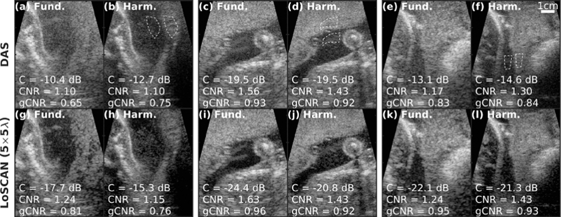
Example fundamental and harmonic in vivo fetal images before (top) and after (bottom) lag-one spatial coherence adaptive normalization (LoSCAN). Contrast, contrast-to-noise ratio (CNR) and generalized CNR (gCNR) for regions of interest, indicated by dashed white lines, are reported in the bottom left of each image. Reprinted, with permission, from Long et al. (2020b).
Another approach to coherence-based beamforming is filtered-delay multiply and sum (F-DMAS), which itself was based on medical microwave imaging techniques (Lim et al. 2008; Matrone et al. 2015). In its original implementation, the signal magnitude in a single scan line is calculated by multiplying the magnitudes of the signals received by each possible array element pair and summing, which is mathematically equivalent to summing the autocorrelation pairs. Matrone et al. scale the output with a signed square root of the multiplied signals so that the resulting amplitude is not dimensionally squared; the full description is
| (32) |
where M is the number of array elements and i is the element index. This output is bandpass filtered to produce the final F-DMAS scan line.
Filtered-delay multiply and sum and a variant employing synthetic transmit aperture focus have been reported to greatly improve contrast, dynamic range and resolution (Matrone et al. 2015, 2017b). Its success prompted the development of short-lag F-DMAS (SL F-DMAS) for use in multiline transmission sequences, where significant off-axis energy is received by array elements far apart on the transducer, that is, large j − 1 (Mallart and Fink 1992; Matrone and Ramalli 2018). DMAS principles can also be extended receive element pairs to the transmit domain; Shen and Hsieh (2019) describe success in improving lateral resolution and contrast with this technique.
Other approaches to coherence-based beamforming use the non-normalized, full covariance matrix, rather than the simplified coherence function in eqn (22). Translating the work of Capon (1969) to ultrasound, Synnevag et al. (2007) describe a method to perform minimum variance (MV) beamforming, which relies on the covariance matrix, to estimate weights that reject noise and interfering signal. The optimized signal for a single scan line in MV beamforming is described as
| (33) |
where L is the number of overlapping apertures contributing to the scan line, w is a complex vector of optimized weights, and si(t) is an array of received signals in elements of the indexed subarray. The weights are estimated from the ensemble covariance matrix over all subarrays, R, as
| (34) |
where a is a steering vector for all subarrays.
Synnevag et al. (2007, 2009) documented the improvements seen with MV beamforming, which include improved contrast, reduced sidelobes and an extension of the depth-of-field. Wang and Li (2009) combined MV beamforming with CF weighting to improve CF estimates in plane wave applications, where the transmit beams are broad and CF estimates are inaccurate. Replacing the numerator in eqn (24) with the known power output of the MV beamforming, the estimate for CF is modified as
| (35) |
Figure 11 illustrates the improvements observed in imaging a breast carcinoma with microcalcifications. Visualization of the microcalcifications, which are small bright targets, is greatly improved with CFMV weighting. The contrast of the breast parenchyma, which is hyperechoic to the surrounding tissue, is also improved. This study and others have found that this method improves key image quality metrics, such as contrast, CNR and resolution (Asl and Mahloojifar 2009; Wang and Li 2014). Like DMAS principles, MV principles can be extended to the transmit domain to produce similar results in boosting contrast and reducing sidelobes (Holfort et al. 2009; Zhao et al. 2015).
Fig. 11.
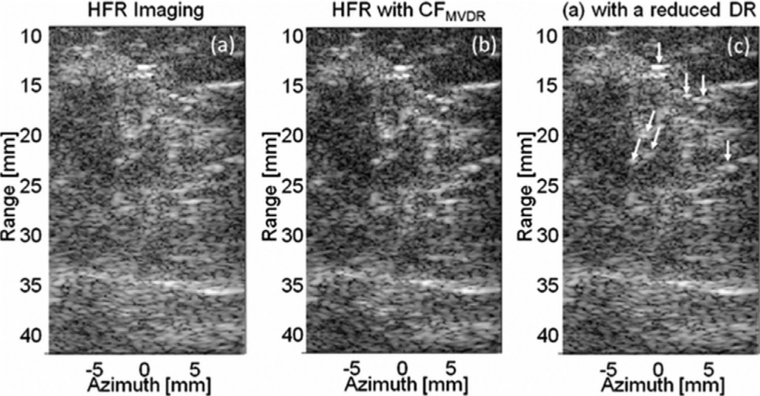
. In vivo images of a breast carcinoma with microcalcifications. (a) High-frame-rate (HFR) B-mode image. (b) B-mode weighted with coherence factor adjusted for minimum variance beamforming (CFMV). (c) Original B-mode with a reduced dynamic range (DR) to match the speckle variance in (b). Microcalcifications are indicated with arrows in (c). Reprinted, with permission, from Wang and Li (2009).
Morgan et al. (2019c) employ the covariance matrix in a model-based approach that rests on the idea that total covariance may be described as the superposition of signal covariance and noise covariance. In their decomposition, three models of covariance are used: mainlobe signal, sidelobe noise and incoherent noise. This method, multicovariate imaging of subresolution targets (MIST), outperforms B-mode in resolution and adherence to native contrast over a range of channel SNR levels (Morgan et al. 2019b). Figure 12 illustrates a comparison of MIST with B-mode, receive spatial compounding and SLSC. In these images, MIST yields the best contrast and high-quality CNR and SNR, while retaining good border definition and resolution that is not seen in the spatial compounding and SLSC cases.
Fig. 12.
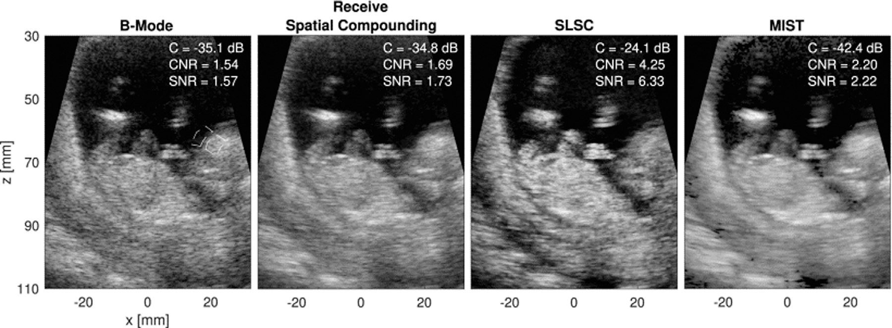
Example in vivo images comparing (left to right) B-mode, receive spatial compounding, short-lag spatial coherence (SLSC) and multicovariate imaging of subresolution targets (MIST). Reprinted, with permission, from Morgan et al. (2019b).
Recent work from Lambert et al. (2020a, 2020b) also investigates the properties of superposition in covariance matrices, but groups non-signal terms in a distortion term and performs a time-reversal analysis of the distortion matrix to unscramble phase aberration over a large field of view. This method greatly improves resolution and point-structure visibility. Though this method, like the other covariance-based methods detailed in this section, is computationally intensive and therefore time consuming, advances in computing power will continue to make these and even more complex future methods more viable in clinical settings.
Spatial coherence as a biomarker
Because of its close relationship to inherent tissue properties such as geometry, compositions and speed of sound, spatial coherence has been used as an imaging biomarker for several clinical applications (Derode and Fink 1993; Anderson et al. 1998; Papadacci et al. 2014, 2017; Imbault et al. 2017, 2018; Wiacek et al. 2020b). Early studies investigated spatial coherence-adjacent properties, such as the speckle correlation length and spatial autocorrelation FWHM (Sehgal and Greenleaf 1984; Anderson et al. 1998). This subsection will detail recent key efforts to advance understanding of the relationship between coherence and tissue properties.
Papadacci et al. (2014) found that coherence may be used to characterize speckle anisotropy in skeletal muscle and myocardium. Their proposed method of doing so, backscatter tensor imaging (BTI), seeks to overcome the long acquisition times needed for magnetic resonance diffusion tensor imaging and ultrasonic shear wave imaging. The premise of BTI is that coherence is maximized when the muscle fiber direction is parallel to the face of a 1-D transducer, because of the coherence length of the backscattered signal along the axis of the fiber. Figure 13 illustrates results corroborating this for a porcine myocardial sample. The authors contend that BTI may be useful in other anisotropic organs such as the brain and tendons, and have determined the feasibility of using a 3-D extension of this method to image the dynamics of cardiac fiber orientation in humans (Papadacci et al. 2017).
Fig. 13.
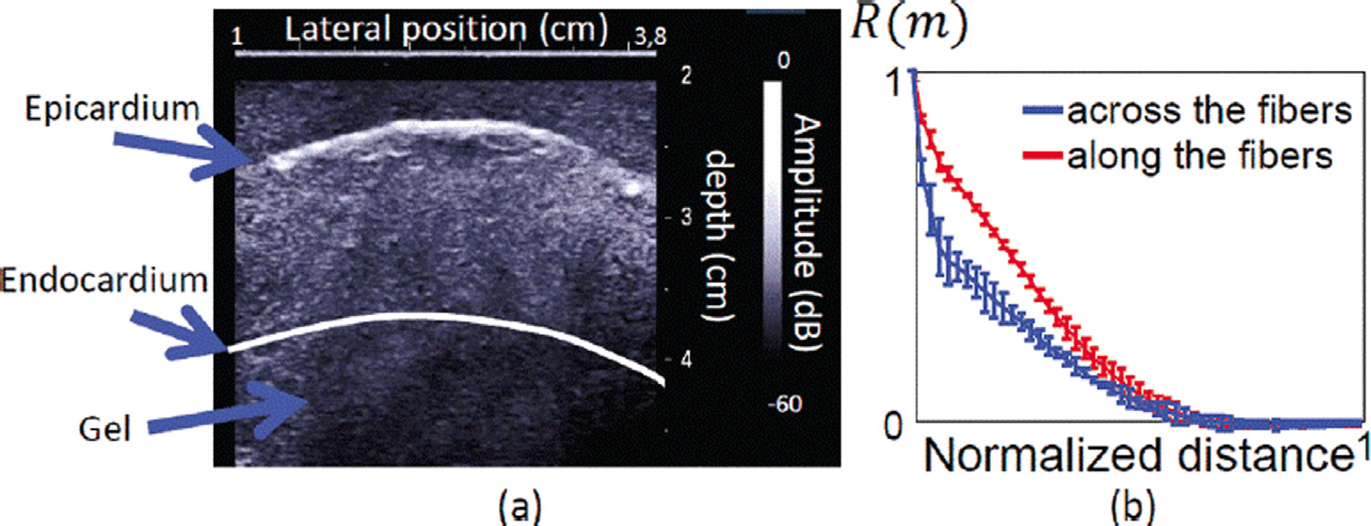
Backscatter tensor imaging in a porcine myocardial sample, with the B-mode image (a) and measured coherence functions (b). Coherence functions across the fibers and along the fibers are in blue and red, respectively. Reprinted, with permission, from Papadacci et al. (2014).
Another application that uses the full coherence curve is sound speed estimation (SSE) for hepatic steatosis assessment (Imbault et al. 2017). Imbault et al. posit that the coherence curve is maximized when the image is beamformed with an assumed sound speed that is closest to that of the liver. By estimating the sound speed with coherence maps generated by beamforming at different sound speeds, the degree of steatosis may be characterized, as there is a well-documented relationship between sound speed and percentage of fat in the liver (Bamber and Hill 1981; Duck 1990). Figure 14 illustrates their results in two patients. The healthy patient, shown on the left, appears to have a higher sound speed than the patient with severe steatosis, shown on the right. The determined sound speed in a patient sample of n = 16 showed good agreement with MRI proton density fat fraction (PDFF) and biopsy results. Imbault et al. (2018) later showed that SSE can provide fat fraction quantification results that are high correlated with MRI PDFF measurements.
Fig. 14.
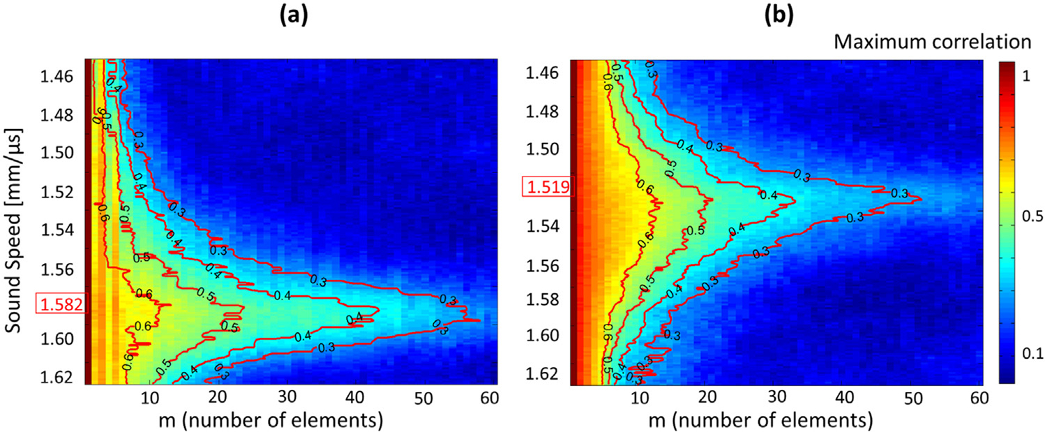
Correlation maps in a healthy patient (a) and a patient with severe steatosis (b). The determined sound speed characterizing the medium is highlighted on the vertical axes. Reprinted, with permission, from Imbault et al. (2017).
Recalling the SLSC beamformer, Wiacek et al. (2020b) found that SLSC may be used to distinguish fluid-filled and solid masses in breast exams, which present with similar echogenicities in standard B-mode images. Presented as an overlay to a B-mode image, SLSC images distinguish solid masses from fluid-filled masses, as solid masses appear more coherent. This work has implications for reducing the percentage of fluid-filled masses being unnecessarily recommended for biopsy; results from presenting the findings to five board-certified radiologists found a reduction in recommendations for these unnecessary biopsies from 43.3% to 13.3%.
DISCUSSION
Limitations
For all its additional insights, the use of spatial coherence is not without limitations. The primary limitation that has held coherence back from broader clinical use is its computational complexity. Consider the processing of an imaging frame from M channels. The number of floating point operations (FLOPs) to perform DAS beamforming is O(M), whereas that for coherence beam-forming is approximately O(nNM) for a calculation using n axial samples and N lags. This can be made further efficient by implementing a single sample calculation as described by eqn (23) for a reduction to O(NM), but the more rigorous coherence-based beamformers that require the full coherence function or covariance matrix still require at least O(M2) FLOPs. These applications include MIST, MV and SLSC with Q = 100% (Synnevag et al. 2007; Lediju et al. 2011; Morgan et al. 2019b).
Modern computer architectures allow for this issue to be partially circumvented. Analysis of coherence-based processing with GPUs has revealed that it is possible to perform real-time SLSC imaging at more than 30 frames per second (fps), an improvement of two orders of magnitude over CPU-based processing (Hyun et al. 2019; Gonzalez and Bell 2020). Though this falls short of frame rates necessary for advanced applications, such as flow imaging, this frame rate represents an accessible baseline to bringing coherence imaging to clinical settings. Additionally, techniques to improve frame rates in such advanced applications are under investigation (Li and Dahl 2015). Furthermore, advances in computer hardware have pushed processing speeds ever faster; clinically relevant frame rates may be achievable with affordable hardware in only a few years.
Another limitation of coherence lies in its method of calculation. For many applications reviewed in this work, an assumption in the calculation is that the source of decorrelation between channel pairs is due to noise independent of the transducer, for example, acoustic clutter. However, there are transducer characteristics that confound the ability of coherence to evaluate image quality in a given window. The most well-documented is bandwidth limitations, leading to amplifications in thermal noise when imaging at the extremes of the transducer bandwidth (Goldberg and Smith 1995; Oakley 1997; Lencioni et al. 2002). In addition, transducers suffer from element non-uniformity, element angular sensitivity and channel crosstalk, all of which introduce irregularities in the received signal and cause decorrelation beyond theoretical predictions (Smith et al. 1992; Zipparo et al. 2004; Ramalli et al. 2015, 2019; Dudley and Woolley 2016). Though transducer design and materials are ever-improving to address these concerns (Zhou et al. 2014; Christiansen et al. 2015), limitations remain.
Lastly, coherence imaging introduces artifacts not seen in B-mode imaging. Though some of these artifacts, such as the dark-region artifact, are well characterized in the literature (Dahl et al. 2017), they are not widely recognizable to sonographers and clinicians unfamiliar with coherence-based techniques. Without proper training to identify and account for these artifacts, the diagnostic power of coherence imaging is limited, even if quantitative improvements in image quality are observed. Furthermore, coherence imaging appears inherently different from B-mode imaging in terms of the presentation of structures, expected dynamic range and resolution. While techniques such as histogram matching may be used to address some of these differences (Bottenus et al. 2021a), there does not exist a comprehensive solution.
On the other hand, early observer studies suggest that clinicians recognize the improvements afforded by coherence, even without a rigorous understanding of the theory or extensive processing to match the appearance of coherence images to B-mode images (Long et al. 2018c; Hyun et al. 2019). Additionally, Rodrigues-Molares et al. (2020) found that coherence beamformers such as SLSC improve target detectability without artificial increases in contrast created by dynamic range distortions introduced by other modern beamformers. The advent of deep learning methods to make clinical diagnoses also suggests that quantitative improvements in image quality may be sufficient for coherence to have key clinical impacts (Jamieson et al. 2012; Cheng et al. 2016; Ma et al. 2016; Ravishankar et al. 2016; Yu et al. 2017). However, a series of recent reviews indicate the ramifications of human-free diagnosis remain under intense investigation (Shen et al. 2017; Litjens et al. 2017; Ker et al. 2018).
Future directions
Despite these limitations, the connectivity and innovation of the medical ultrasound community present several exciting opportunities to further expand the role of spatial coherence. Rodriguez-Molares et al. (2017) presented the UltraSound ToolBox (USTB), a framework for standardizing ultrasound signal processing that includes a module to perform SLSC beamforming and makes coherence processing widely accessible and shareable. The explosion of deep learning methods in medical imaging has also found use in improving the computational efficiency in coherence calculations. Wiacek et al. (2020a) found that their deep neural network, CohereNet, improved processing speeds beyond CPU-based approaches. Additionally, manufacturers of diagnostic scanners currently implement beamforming and image formation strategies related to coherence or have hardware that would support the data storage and number of calculations necessary for coherence applications (Thiele et al. 2013; Loftman 2017; GE Healthcare 2019). In particular, Siemens describes a technique by which retrospective transmit focusing is employed to maximize the coherence factor (Loftman 2017). Additionally, GE and Philips employ parallel computing strategies that enable processing of large amounts of data (Thiele et al. 2013; GE Healthcare 2019). This suggests that many of the techniques discussed in this review and future ones could be readily implemented on diagnostic scanners.
There also exist several possibilities to pair principles of coherence with other modern approaches to medical ultrasound. Advances in acquisition techniques, such as ultrafast plane wave imaging, diverging wave imaging and multiline transmission, have proven to be amenable to coherence applications (Camacho et al. 2009; Matrone and Ramalli 2018; Matrone et al. 2017a, 2020; Turquin et al. 2017). Synthetic aperture beam-forming, employed to improve focusing among other image quality factors, has also been combined with coherence imaging to great success (Bottenus et al. 2013; Morgan et al. 2020). Beamforming geometries may be further expanded into the third dimension, as indicated by several groups who have measured spatial coherence over an elevational extent to better estimate signal-to-clutter levels (Fatemi et al. 2020; Hansen-Shearer et al. 2022; Ahmed et al. 2022). As processing techniques, coherence based or otherwise, have improved, ultrasound imaging finds itself in new terrain previously thought as not amenable to acoustics. The bulk of literature exploring coherence has focused on abdominal applications, where signal attenuation is minimal and speckle is well developed in large homogeneous regions, but advances in hardware and processing techniques have opened up new possibilities for image quality characterization in transcranial applications (Vienneau et al. 2020).
Lastly, inspiration may be drawn from related fields, such as sonar, astronomy and medical optics, to find novels ways of implementing coherence in ultrasound. The abundance of literature in these other fields suggests that the ultrasound community has only scratched the surface of coherence-based techniques (Pearson and Readhead 1984; Pinto et al. 1997; Gori et al. 2000; de Boer et al. 2003; Dorrer 2004; Yaqoob et al. 2005; D’Spain et al. 2006; Carozzi and Woan 2009; Hansen et al. 2011; Li et al. 2013). For example, the spatial coherence of reverberated echoes from the seafloor has been used to autofocus synthetic apertures in sonar, a technique with no current analogue in ultrasound (Pinto et al. 1997; Hansen et al. 2011). In a medically relevant example, evaluation of the spectral coherence, rather than time-domain coherence, in optical coherence tomography (OCT) has helped improved the SNR by over two orders of magnitude (de Boer et al. 2003; Yaqoob et al. 2005).
CONCLUSIONS
Decades of work in spatial coherence in medical ultrasound have yielded numerous advances in beamforming, image quality characterization and tissue characterization. These advances promise to greatly expand the capabilities of ultrasound in clinical settings by improving the standard of image-based diagnoses and introducing new measures by which to make clinical judgments. As the implementation of these techniques becomes more efficient and accelerated by improved computer hardware, spatial coherence will become more clinically feasible as an addition or substitute to standard B-mode imaging. An abundance of future work remains, partially guided by advances in other fields such as sonar and OCT.
Acknowledgments—
The authors are indebted to the many scientists whose work serves as the foundation for all current and future studies in coherence. The authors also thank D. Hyun, R. Ahmed and D. Bradway for their insightful comments and suggestions.
This work was funded by National Institutes of Health grants R01-EB026574 and R01-EB017711 from the National Institute of Biomedical Imaging and Bioengineering and the National Science Foundation Graduate Research Fellowship Program.
REFERENCES
- Adler L, Hiedemann EA. Determination of the nonlinearity parameter B/A for water and m-xylene. J Acoust Soc Am 1962;34:410–412. [Google Scholar]
- Ahmed R, Bottenus N, Long J, Trahey GE. Reverberation clutter suppression using 2-D spatial coherence analysis. IEEE Trans Ultrason Ferroelectr Freq Control 2022;69:84–97. [DOI] [PMC free article] [PubMed] [Google Scholar]
- Anderson ME, Soo MSC, Trahey GE. Microcalcifications as elastic scatterers under ultrasound. IEEE Trans Ultrason Ferroelectr Freq Control 1998;45:925–934. [DOI] [PubMed] [Google Scholar]
- Asl BM, Mahloojifar A. Minimum variance beamforming combined with adaptive coherence weighting applied to medical ultrasound imaging. IEEE Trans Ultrason Ferroelectr Freq Control 2009;56:1923–1931. [DOI] [PubMed] [Google Scholar]
- Bamber JC, Hill CR. Acoustic properties of normal and cancerous human liver-I. Dependence on pathological condition. Ultrasound Med Biol 1981;7:121–133. [DOI] [PubMed] [Google Scholar]
- Bamber JC, Mucci RA, Orofino DP. Spatial coherence and beamformer gain. Acoust Imaging 2002;24:43–48. [Google Scholar]
- Bell MAL, Kuo NP, DYS MD, Kang JU, Boctor EM. In vivo visualization of prostate brachytherapy seeds with photoacoustic imaging. J Biomed Opt 2014;19:1–13. [DOI] [PMC free article] [PubMed] [Google Scholar]
- Bottenus NB, Trahey GE. Equivalence of time and aperture domain additive noise in ultrasound coherence. J Acoust Soc Am 2015;137:132–138. [DOI] [PMC free article] [PubMed] [Google Scholar]
- Bottenus N, Ustüner KF. Acoustic reciprocity of spatial coherence in ultrasound imaging. IEEE Trans Ultrason Ferroelectr Freq Control 2015;62:852–861. [DOI] [PMC free article] [PubMed] [Google Scholar]
- Bottenus N, Byram BC, Dahl JJ, Trahey GE. Synthetic aperture focusing for short-lag spatial coherence imaging. IEEE Trans Ultrason Ferroelectr Freq Control 2013;60:1816–1826. [DOI] [PMC free article] [PubMed] [Google Scholar]
- Bottenus N, Pinton GF, Trahey G. The impact of acoustic clutter on large array abdominal imaging. IEEE Trans Ultrason Ferroelectr Freq Control 2020;67:703–714. [DOI] [PMC free article] [PubMed] [Google Scholar]
- Bottenus N, Byram BC, Hyun D. Histogram matching for visual ultrasound image comparison. IEEE Trans Ultrason Ferroelectr Freq Control 2021a;68:1487–1495. [DOI] [PMC free article] [PubMed] [Google Scholar]
- Bottenus N, Straube T, Farling S, Vesel T, Klitzman B, Deshusses MA, Cheifetz IM. Ultrasonic bubble detection and tracking using spatial coherence and motion modeling. Medical Imaging 2021;. doi: 10.1117/12.2580587 Ultrasonic Imaging and Tomography; 116020F (2021).. [DOI] [Google Scholar]
- Burckhardt CB. Speckle in ultrasound B-mode scans. IEEE Trans Sonics Ultrason 1978;25:1–6. [Google Scholar]
- Byram B, Dei K, Tierney J, Dumont D. A model and regularization scheme for ultrasonic beamforming clutter reduction. IEEE Trans Ultrason Ferroelectr Freq Control 2015;62:1913–1927. [DOI] [PMC free article] [PubMed] [Google Scholar]
- Camacho J, Parrilla M, Fritsch C. Phase coherence imaging. IEEE Trans Ultrason Ferroelectr Freq Control 2009;56:958–974. [DOI] [PubMed] [Google Scholar]
- Capon J High-resolution frequency-wavenumber spectrum analysis. Proc IEEE 1969;57:1408–1418. [Google Scholar]
- Carozzi TD, Woan G. A generalized measurement equation and van Cittert-Zernike theorem for wide-field radio astronomical interferometry. Mon Not R Astron Soc 2009;395:1558–1568. [Google Scholar]
- Cheng JZ, Ni D, Chou YH, Qin J, Tiu CM, Chang YC, Huang CS, Shen D, Chen CM. Computer-aided diagnosis with deep learning architecture: Applications to breast lesions in US images and pulmonary nodules in CT scans. Sci Rep 2016;6:24454. [DOI] [PMC free article] [PubMed] [Google Scholar]
- Christiansen TL, Jensen JA, Thomsen EV. Acoustical cross-talk in row-column addressed 2-D transducer arrays for ultrasound imaging. Ultrasonics 2015;63:174–178. [DOI] [PubMed] [Google Scholar]
- D’Spain GL, Luby JC, Wilson GR, Gramann RA. Vector sensors and vector sensor line arrays: Comments on optimal array gain and detection. J Acoust Soc Am 2006;120:171–185. [Google Scholar]
- Dahl JJ, Sheth NM. Reverberation clutter from subcutaneous tissue layers: Simulation and in vivo demonstrations. Ultrasound Med Biol 2014;40:714–726. [DOI] [PMC free article] [PubMed] [Google Scholar]
- Dahl JJ, Hyun D, Lediju M, Trahey GE. Lesion detectability in diagnostic ultrasound with short-lag spatial coherence imaging. Ultrason Imaging 2011;33:119–133. [DOI] [PMC free article] [PubMed] [Google Scholar]
- Dahl JJ, Jakovljevic M, Pinton GF, Trahey GE. Harmonic spatial coherence imaging: An ultrasonic imaging method based on backscatter coherence. IEEE Trans Ultrason Ferroelectr Freq Control 2012;59:648–659. [DOI] [PMC free article] [PubMed] [Google Scholar]
- Dahl JJ, Hyun D, Li Y, Jakovljevic M, Bell MAL, Long WJ, Bottenus N, Kakkad V, Trahey GE. Coherence beamforming and its applications to the difficult-to-image patient. Proc IEEE Int Ultrason Symp 2017;1–10. [Google Scholar]
- de Boer JF, Cense B, Park BH, Pierce MC, Tearney GJ, Bouma BE. Improved signal-to-noise ratio in spectral-domain compared with time-domain optical coherence tomography. Opt Lett 2003;28:2067–2069. [DOI] [PubMed] [Google Scholar]
- Derode A, Fink M. Spatial coherence of ultrasonic speckle in composites. IEEE Trans Ultrason Ferroelectr Freq Control 1993;40:666–675. [DOI] [PubMed] [Google Scholar]
- Dorrer C Temporal van Cittert-Zernike theorem and its application to the measurement of chromatic dispersion. J Opt Soc Am B 2004;21:1417–1423. [Google Scholar]
- Duck FA. Acoustic properties of tissue at ultrasonic frequencies. London: Academic Press; 1990. p. 73–135. [Google Scholar]
- Dudley NJ, Woolley DJ. A simple uniformity test for ultrasound phased arrays. Phys Med 2016;32:1162–1166. [DOI] [PubMed] [Google Scholar]
- Fatemi A, Berg EAR. Rodriguez-Molares A. Studying the origin of reverberation clutter in echocardiography: In vitro experiments and in vivo demonstrations. Ultrasound Med Biol 2019;45:1799–1813. [DOI] [PubMed] [Google Scholar]
- Fatemi A, Måsøy SE. Rodriguez-Molares A. Row-column-based coherence imaging using a 2-D array transducer: A row-based implementation. IEEE Trans Ultrason Ferroelectr Freq Control 2020;67:2303–2311. [DOI] [PubMed] [Google Scholar]
- Fedewa RJ, Wallace KD, Holland MR, Jago JR, Ng GC, Rielly MR, Robinson BS, Miller JG. Spatial coherence of the nonlinearly generated second harmonic portion of backscatter for a clinical imaging system. IEEE Trans Ultrason Ferroelectr Freq Control 2003;50:1010–1022. [DOI] [PubMed] [Google Scholar]
- Fink M Time reversal of ultrasonic fields. I. Basic principles. IEEE Trans Ultrason Ferroelectr Freq Control 1992;39:555–566. [DOI] [PubMed] [Google Scholar]
- Fink MA, Cardoso JF. Diffraction Effects in Pulse-Echo Measurement. IEEE Trans Sonics Ultrason 1984;31:313–329. [Google Scholar]
- Flint K, Bottenus N, Bradway D, McNally P, Ellestad S, Trahey G. An Automated ALARA method for ultrasound. J Ultrasound Med 2021;40:1863–1877. [DOI] [PMC free article] [PubMed] [Google Scholar]
- Freiburger PD, Sullivan DC, LeBlanc BH, Smith SW, Trahey GE. Two dimensional ultrasonic beam distortion in the breast: In vivo measurements and effects. Ultrason Imaging 1992;14:398–414. [DOI] [PubMed] [Google Scholar]
- GE Healthcare. White paper: cSound 3.0 Taking the processing power and patient care advantages to a new level with artificial intelligence. Technical report, 2019. [Google Scholar]
- Goldberg RL, Smith SW. Optimization of signal-to-noise ratio for multilayer pzt transducers. Ultrason Imaging 1995;17:95–113. [DOI] [PubMed] [Google Scholar]
- Gonzalez EA, Bell MAL. GPU implementation of photoacoustic short-lag spatial coherence imaging for improved image-guided interventions. J Biomed Opt 2020;25:1–19. [DOI] [PMC free article] [PubMed] [Google Scholar]
- Goodman JW. Statistical optics. 2nd edition New York: Wiley; 2015. [Google Scholar]
- Gori F, Santarsiero M, Borghi R, Piquero G. Use of the van CittertZernike theorem for partially polarized sources. Opt Lett 2000;25:1291–1293. [DOI] [PubMed] [Google Scholar]
- Graham MT, Bell MAL. Photoacoustic spatial coherence theory and applications to coherence-based image contrast and resolution. IEEE Trans Ultrason Ferroelectr Freq Control 2020;67:2069–2084. [DOI] [PMC free article] [PubMed] [Google Scholar]
- Hall TJ, Insana MF, Soller NM, Harrison LA. Ultrasound contrast-detail analysis: A preliminary study in human observer performance. Med Phys 1993;20:117–127. [DOI] [PubMed] [Google Scholar]
- Hansen RE, Callow HJ, Sabo TO, Synnes SAV. Challenges in seafloor imaging and mapping with synthetic aperture sonar. IEEE Trans Geosci Remote Sensing 2011;49:3677–3687. [Google Scholar]
- Hansen-Shearer J, Lerendegui M, Toulemonde M, Tang MX. Ultrafast 3-D ultrasound imaging using row-column array-specific framemultiply-and-sum beamforming. IEEE Trans Ultrason Ferroelectr Freq Control 2022;69:480–488. [DOI] [PubMed] [Google Scholar]
- Hendler I, Blackwell SC, Bujold E, Treadwell MC, Wolfe HM, Sokol RJ, Sorokin Y. The impact of maternal obesity on midtrimester sonographic visualization of fetal cardiac and craniospinal structures. Int J Obesity 2004;28:1607–1611. [DOI] [PubMed] [Google Scholar]
- Hinkelman LM, Liu D, Metlay LA, Waag RC. Measurements of ultrasonic pulse arrival time and energy level variations produced by propagation through abdominal wall. J Acoust Soc Am 1994;95:530–541. [DOI] [PubMed] [Google Scholar]
- Hinkelman LM, Liu D, Waag RC, Zhu Q, Steinberg BD. Measurement and correction of ultrasonic pulse distortion produced by the human breast. J Acoust Soc Am 1995;97:1958–1969. [DOI] [PubMed] [Google Scholar]
- Hinkelman LM, Mast TD, Metlay LA, Waag RC. The effect of abdominal wall morphology on ultrasonic pulse distortion. Part I. Measurements. J Acoust Soc Am 1998;104:3635–3649. [DOI] [PubMed] [Google Scholar]
- Holfort IK, Austeng A, Synnevag JF, Holm S, Gran F, Jensen JA. Adaptive receive and transmit apodization for synthetic aperture ultrasound imaging. In: Proc 2009 IEEE Int Ultrason Symp. 1–4. [Google Scholar]
- Hollman KW, Rigby KW, O’Donnell M. Coherence factor of speckle from a multi-row probe. 1999. IEEE Ultrasonics Symposium. Proc IEEE Int Symp. 2, 1257–1260. [Google Scholar]
- Hyun D, Trahey GE, Jakovljevic M, Dahl JJ. Short-lag spatial coherence imaging on matrix arrays: Part 1. Beamforming methods and simulation studies. IEEE Trans Ultrason Ferroelectr Freq Control 2014;61:1101–1112. [DOI] [PMC free article] [PubMed] [Google Scholar]
- Hyun D, Crowley ALC, Dahl JJ. Efficient Strategies for Estimating the Spatial Coherence of Backscatter. IEEE Trans Ultrason Ferroelectr Freq Control 2017;64:500–513. [DOI] [PMC free article] [PubMed] [Google Scholar]
- Hyun D, Abou-Elkacem L, Perez VA, Chowdhury SM, Willmann JK, Dahl JJ. Improved sensitivity in ultrasound molecular imaging with coherence-based beamforming. IEEE Trans Med Imaging 2018;37:214–250. [DOI] [PMC free article] [PubMed] [Google Scholar]
- Hyun D, Crowley ALC, LeFevre M, Cleve J, Rosenberg J, Dahl JJ. Improved visualization in difficult-to-image stress echocardiography patients using real-time harmonic spatial coherence imaging. IEEE Trans Ultrason Ferroelectr Freq Control 2019;66:433–441. [DOI] [PMC free article] [PubMed] [Google Scholar]
- Hyun D, Dahl JJ. Effects of motion on correlations of pulse-echo ultrasound signals: Applications in delay estimation and aperture coherence. J Acoust Soc Am 2020;147:1323. [DOI] [PMC free article] [PubMed] [Google Scholar]
- Imbault M, Faccinetto A, Osmanski BF, Tissier A, Deffieux T, Gennisson JL, Vilgrain V, Tanter M. Robust sound speed estimation for ultrasound-based hepatic steatosis assessment. Phys Med Biol 2017;62:3582–3598. [DOI] [PubMed] [Google Scholar]
- Imbault M, Dioguardi Burgio M, Faccinetto A, Ronot M, Bendjador H, Deffieux T, Triquet EO, Rautou PE, Castera L, Gennisson JL, Vilgrain V, Tanter M. Ultrasonic fat fraction quantification using in vivo adaptive sound speed estimation. Phys Med Biol 2018;63 215013. [DOI] [PubMed] [Google Scholar]
- Irshad A, Anis M, Ackerman SJ. Current Role of Ultrasound in chronic liver disease: Surveillance, diagnosis and management of hepatic neoplasms. Curr Prob Diagn Radiol 2012;41:43–51. [DOI] [PubMed] [Google Scholar]
- Jakovljevic M, Trahey GE, Nelson RC, Dahl JJ. In vivo application of short-lag spatial coherence imaging in human liver. Ultrasound Med Biol 2013;39:534–542. [DOI] [PMC free article] [PubMed] [Google Scholar]
- Jakovljevic M, Byram BC, Hyun D, Dahl JJ, Trahey GE. Short-lag spatial coherence imaging on matrix arrays, Part II: Phantom and in vivo experiments. IEEE Trans Ultrason Ferroelectr Freq Control 2014;61:1113–1122. [DOI] [PMC free article] [PubMed] [Google Scholar]
- Jakovljevic M, Yoon BC, Abou-Elkacem L, Hyun D, Li Y, Rubesova E, Dahl JJ. Blood flow imaging in the neonatal brain using angular coherence power Doppler. IEEE Trans Ultrason Ferroelectr Freq Control 2021;68:92–106. [DOI] [PMC free article] [PubMed] [Google Scholar]
- Jamieson AR, Drukker K, Giger ML. Breast image feature learning with adaptive deconvolutional networks. Proceedings Volume 8315, Medical Imaging 2012: Computer-Aided Diagnosis 2012;831506. doi: 10.1117/12.910710. [DOI] [Google Scholar]
- Karaman M, Atalar A, Koymen H, O’Donnell M. A phase aberration correction method for ultrasound imaging. IEEE Trans Ultrason Ferroelectr Freq Control 1993;40:275–282. [DOI] [PubMed] [Google Scholar]
- Kasai C, Namekawa K. Real-time two-dimensional blood flow imaging using an autocorrelation technique. Proc IEEE Int Ultrason Symp 1985;953–958. [Google Scholar]
- Ker J, Wang L, Rao J, Lim T. Deep learning applications in medical image analysis. IEEE Access 2018;6:9375–9389. [Google Scholar]
- Khoury FR, Khoury FR, Ehrenberg HM, Mercer BM. The impact of maternal obesity on satisfactory detailed anatomic ultrasound image acquisition. J Matern Fetal Neonatal Med 2009;22:337–341. [DOI] [PubMed] [Google Scholar]
- Kremkau FW, Taylor KJ. Artifacts in ultrasound imaging. J Ultrasound Med 1986;5:227–237. [DOI] [PubMed] [Google Scholar]
- Krishnan S, Li PC, O’Donnell M. Adaptive compensation of phase and magnitude aberrations. IEEE Trans Ultrason Ferroelectr Freq Control 1996;43:44–55. [Google Scholar]
- Krishnan S, Rigby KW, O’Donnell M. Adaptive aberration correction of abdominal images using PARCA. Ultrason Imaging 1997;19:169–179. [DOI] [PubMed] [Google Scholar]
- Lambert W, Cobus LA, Couade M, Fink M, Aubry A. Reflection matrix approach for quantitative imaging of scattering media. Phys Rev X 2020a;10:21048. [Google Scholar]
- Lambert W, Cobus LA, Frappart T, Fink M, Aubry A. Distortion matrix approach for ultrasound imaging of random scattering media. Proc Natl Acad Sci USA 2020b;117:14645–14656. [DOI] [PMC free article] [PubMed] [Google Scholar]
- Lediju MA, Pihl MJ, Dahl JJ, Trahey GE. Quantitative assessment of the magnitude, impact and spatial extent of ultrasonic clutter. Ultrason Imaging 2008;30:151–168. [DOI] [PMC free article] [PubMed] [Google Scholar]
- Lediju MA, Trahey GE, Byram BC, Dahl JJ. Short-lag spatial coherence of backscattered echoes: Imaging characteristics. IEEE Trans Ultrason Ferroelectr Freq Control 2011;58:1377–1388. [DOI] [PMC free article] [PubMed] [Google Scholar]
- Lediju Bell MA, Goswami R, Kisslo JA, Dahl JJ, Trahey GE. Short-lag spatial coherence imaging of cardiac ultrasound data: Initial clinical results. Ultrasound Med Biol 2013a;39:1861–1874. [DOI] [PMC free article] [PubMed] [Google Scholar]
- Lediju Bell MA, Kuo N, Song DY, Boctor EM. Short-lag spatial coherence beamforming of photoacoustic images for enhanced visualization of prostate brachytherapy seeds. Biomed Opt Express 2013b;4:1964–1977. [DOI] [PMC free article] [PubMed] [Google Scholar]
- Lediju Bell MA, Dahl JJ, Trahey GE. Resolution and brightness characteristics of short-lag spatial coherence (SLSC) images. IEEE Trans Ultrason Ferroelectr Freq Control 2015;62:1265–1276. [DOI] [PMC free article] [PubMed] [Google Scholar]
- Ledoux LAF, Brands PJ, Hoeks APG. Reduction of the clutter component in Doppler ultrasound signals based on singular value decomposition: A simulation study. Ultrason Imaging 1997;19:1–18. [DOI] [PubMed] [Google Scholar]
- Lencioni R, Cioni D, Bartolozzi C. Tissue harmonic and contrast-specific imaging: Back to gray scale in ultrasound. Eur Radiol 2002;12:151–165. [DOI] [PubMed] [Google Scholar]
- Li PC, Li ML. Adaptive imaging using the generalized coherence factor. IEEE Trans Ultrason Ferroelectr Freq Control 2003;50:128–141. [DOI] [PubMed] [Google Scholar]
- Li YL, Dahl JJ. Coherent flow power doppler (CFPD): Flow detection using spatial coherence beamforming. IEEE Trans Ultrason Ferroelectr Freq Control 2015;62:1022–1035. [DOI] [PMC free article] [PubMed] [Google Scholar]
- Li YL, Dahl JJ. Angular coherence in ultrasound imaging: Theory and applications. J Acoust Soc Am 2017;141:1582–1594. [DOI] [PMC free article] [PubMed] [Google Scholar]
- Li J, Zhang X, Gao X. A joint scheme for angle and array gain-phase error estimation in bistatic MIMO radar. IEEE Geosci Remote Sensing Lett 2013;10:1478–1482. [Google Scholar]
- Li YL, Hyun D, Abou-Elkacem L, Willmann JK, Dahl JJ. Visualization of small-diameter vessels by reduction of incoherent reverberation with coherent flow power Doppler. IEEE Trans Ultrason Ferroelectr Freq Control 2016;63:1878–1889. [DOI] [PMC free article] [PubMed] [Google Scholar]
- Lim HB, Nhung NTT, Li EP, Thang ND. Confocal microwave imaging for breast cancer detection: Delay-multiply-and-sum image reconstruction algorithm. IEEE Trans on Biomed Eng 2008;55:1697–1704. [DOI] [PubMed] [Google Scholar]
- Litjens G, Kooi T, Bejnordi BE, Setio AAA, Ciompi F, Ghafoorian M, van der Laak JAWM, van Ginneken B, Sánchez CI. A survey on deep learning in medical image analysis. Med Image Anal 2017;42:60–88. [DOI] [PubMed] [Google Scholar]
- Liu D, Waag RC. Correction of ultrasonic wavefront distortion using backpropagation and a reference waveform method for time-shift compensation. J Acoust Soc Am 1994;96:649–660. [DOI] [PubMed] [Google Scholar]
- Liu DL, Waag RC. About the application of the van Cittert-Zernike theorem in ultrasonic imaging. IEEE Trans Ultrason Ferroelectr Freq Control 1995;42:590–601. [Google Scholar]
- Loftman R. White paper: IN Focus Coherent Technology. Technical report. Siemens Medical Solutions, 2017. [Google Scholar]
- Long J, Long W, Bottenus N, Pinton GF, Trahey GE. Implications of lag-one coherence on real- time adaptive frequency selection. Proc IEEE Int Ultrason Symp 2018;1–9. [Google Scholar]
- Long W, Bottenus N, Trahey GE. Lag-one coherence as a metric for ultrasonic image quality. IEEE Trans Ultrason Ferroelectr Freq Control 2018b;65:1768–1780. [DOI] [PMC free article] [PubMed] [Google Scholar]
- Long W, Hyun D, Choudhury KR, Bradway D, McNally P, Boyd B, Ellestad S, Trahey GE. Clinical utility of fetal short-lag spatial coherence imaging. Ultrasound Med Biol 2018c;44:794–806. [DOI] [PMC free article] [PubMed] [Google Scholar]
- Long J, Long W, Bottenus N, Trahey G. Coherence-based quantification of acoustic clutter sources in medical ultrasound. J Acoust Soc Am 2020a;148:1051–1062. [DOI] [PMC free article] [PubMed] [Google Scholar]
- Long W, Bottenus N, Trahey GE. Incoherent clutter suppression using lag-one coherence. IEEE Trans Ultrason Ferroelectr Freq Control 2020;67:1554–1557. [DOI] [PMC free article] [PubMed] [Google Scholar]
- Ma J, Wu F, Zhu J, Xu D, Kong D. A pre-trained convolutional neural network based method for thyroid nodule diagnosis. Ultrasonics 2016;73:221–230. [DOI] [PubMed] [Google Scholar]
- Mallart R, Fink M. The van Cittert-Zernike theorem in pulse echo measurements. J Acoust Soc Am 1991;90:2718–2727. [Google Scholar]
- Mallart R, Fink M. Improved imaging rate through simultaneous transmission of several ultrasound beams. In: Proceedings Volume 1733. New developments in ultrasonic transducers and transducer systems. 1992. doi: 10.1117/12.130591. [DOI] [Google Scholar]
- Mallart R, Fink M. Adaptive focusing in scattering media through sound-speed inhomogeneities: The van Cittert Zernike approach and focusing criterion. J Acoust Soc Am 1994;96:3721–3732. [Google Scholar]
- Måsøy SE, Varslot T, Angelsen B. Iteration of transmit-beam aberration correction in medical ultrasound imaging. J Acoust Soc Am 2005;117:450–461. [DOI] [PubMed] [Google Scholar]
- Mast TD, Hinkelman LM, Orr MJ, Sparrow VW, Waag RC. Simulation of ultrasonic pulse propagation through the abdominal wall. J Acoust Soc Am 1997;102:1177–1190. [DOI] [PubMed] [Google Scholar]
- Mast TD, Hinkelman LM, Orr MJ, Waag RC. The effect of abdominal wall morphology on ultrasonic pulse distortion. Part II. Simulations. J Acoust Soc Am 1998;104:3651–3664. [DOI] [PubMed] [Google Scholar]
- Matrone G, Ramalli A. Spatial coherence of backscattered signals in multi-line transmit ultrasound imaging and its effect on short-lag filtered-delay multiply and sum beamforming. Appl Sci 2018;8:486. [Google Scholar]
- Matrone G, Savoia AS, Caliano G, Magenes G. The delay multiply and sum beamforming algorithm in ultrasound B-mode medical imaging. IEEE Trans Med Imaging 2015;34:940–949. [DOI] [PubMed] [Google Scholar]
- Matrone G, Ramalli A, Savoia AS, Tortoli P, Magenes G. High frame-rate, high resolution ultrasound imaging with multi-line transmission and filtered-delay multiply and sum beamforming. IEEE Trans Med Imaging 2017a;36:478–486. [DOI] [PubMed] [Google Scholar]
- Matrone G, Savoia AS, Caliano G, Magenes G. Depth-of-field enhancement in filtered-delay multiply and sum beamformed images using synthetic aperture focusing. Ultrasonics 2017b;75:216–225. [DOI] [PubMed] [Google Scholar]
- Matrone G, Ramalli A, Dhooge J, Tortoli P, Magenes G. A comparison of coherence-based beamforming techniques in high-frame-rate ultrasound imaging with multi-line transmission. IEEE Trans Ultrason Ferroelectr Freq Control 2020;67:329–340. [DOI] [PubMed] [Google Scholar]
- Matrone G, Bell MAL, Ramalli A. Spatial coherence beamforming with multi-line transmission to enhance the contrast of coherent structures in ultrasound images degraded by acoustic clutter. IEEE Trans Ultrason Ferroelectr Freq Control 2021;68:3570–3582. [DOI] [PubMed] [Google Scholar]
- Michelson AA. On the application of interference methods to astronomical measurements. London Edinburgh Dublin Philos Mag J Sci 1890;30:1–21. [DOI] [PMC free article] [PubMed] [Google Scholar]
- Morgan MR, Hyun D, Trahey GE. Short-lag spatial coherence imaging in 1.5-D and 1.75-D arrays: Elevation performance and array design considerations. IEEE Trans Ultrason Ferroelectr Freq Control 2019a;66:1047–1056. [DOI] [PMC free article] [PubMed] [Google Scholar]
- Morgan MR, Trahey GE, Walker WF. Multi-covariate imaging of sub-resolution targets. IEEE Trans Med Imaging 2019b;38:1690–1700. [DOI] [PMC free article] [PubMed] [Google Scholar]
- Morgan MR, Trahey GE, Walker WF. Speckle coherence of piecewise-stationary stochastic targets. J Acoust Soc Am 2019c;146:1721–1731. [DOI] [PMC free article] [PubMed] [Google Scholar]
- Morgan MR, Bottenus N, Trahey GE, Walker WF. Synthetic aperture focusing for multi-covariate imaging of sub-resolution targets. IEEE Trans Ultrason Ferroelectr Freq Control 2020;67:1166–1177. [DOI] [PMC free article] [PubMed] [Google Scholar]
- Nair AA, Tran TD, Bell MAL. Robust short-lag spatial coherence imaging. IEEE Trans Ultrason Ferroelectr Freq Control 2018;65:366–377. [DOI] [PMC free article] [PubMed] [Google Scholar]
- Napolitano D, Chou CH, McLaughlin G, Ji TL, Mo L, DeBusschere D, Steins R. Sound speed correction in ultrasound imaging. Ultrasonics 2006;44:e43–e46. [DOI] [PubMed] [Google Scholar]
- Nilsen CC, Holm S. Wiener beamforming and the coherence factor in ultrasound imaging. IEEE Trans Ultrason Ferroelectr Freq Control 2010;57:1329–1346. [DOI] [PubMed] [Google Scholar]
- Nock L, Trahey GE, Smith SW. Phase aberration correction in medical ultrasound using speckle brightness as a quality factor. J Acoust Soc Am 1989;85:1819–1833. [DOI] [PubMed] [Google Scholar]
- Nyborg WL. Biological effects of ultrasound: development of safety guidelines: Part I: personal histories. Ultrasound Med Biol 2000;26:911–964. [DOI] [PubMed] [Google Scholar]
- Oakley CG. Calculation of ultrasonic transducer signal-to-noise ratios using the KLM model. IEEE Trans Ultrason Ferroelectr Freq Control 1997;44:1018–1026. [Google Scholar]
- O’Donnell M, Flax SW. Phase aberration measurements in medical ultrasound: Human studies. Ultrason Imaging 1988;10:1–11. [DOI] [PubMed] [Google Scholar]
- Offerdahl K, Huber M, Long J, Long W, Bottenus N, Trahey G. Occult regions of suppressed coherence in ultrasonic liver images. J Acoust Soc Am 2020;148:2487. [Google Scholar]
- Ozgun K, Tierney J, Byram B. A spatial coherence beamformer design for power Doppler imaging. IEEE Trans Med Imaging 2020;39:1558–1570. [DOI] [PMC free article] [PubMed] [Google Scholar]
- Papadacci C, Tanter M, Pernot M, Fink M. Ultrasound backscatter tensor imaging (BTI): Analysis of the spatial coherence of ultrasonic speckle in anisotropic soft tissues. IEEE Trans Ultrason Ferroelectr Freq Control 2014;61:986–996. [DOI] [PMC free article] [PubMed] [Google Scholar]
- Papadacci C, Finel V, Provost J, Villemain O, Bruneval P, Gennisson JL, Tanter M, Fink M, Pernot M. Imaging the dynamics of cardiac fiber orientation in vivo using 3D ultrasound backscatter tensor imaging. Sci Rep 2017;7:830. [DOI] [PMC free article] [PubMed] [Google Scholar]
- Patterson MS, Foster FS. The improvement and quantitative assessment of B-mode images produced by an annular array/cone hybrid. Ultrason Imaging 1983;5:195–213. [DOI] [PubMed] [Google Scholar]
- Pearson TJ, Readhead ACS. Image formation by self-calibration in radio astronomy. Annu Rev Astron Astrophys 1984;22:97–130. [Google Scholar]
- Pinto MA, Fohanno F, Tremois O, Guyonic S. Autofocusing a synthetic aperture sonar using the temporal and spatial coherence of seafloor reverberation. High Frequency Seafloor Acoustics (SACLANTCEN Conference Proceedings CP-45). 417–424. [Google Scholar]
- Pinton GF, Trahey GE, Dahl JJ. Sources of image degradation in fundamental and harmonic ultrasound imaging using nonlinear, full-wave simulations. IEEE Trans Ultrason Ferroelectr Freq Control 2011;58:754–765. [DOI] [PMC free article] [PubMed] [Google Scholar]
- Pinton GF, Trahey GE, Dahl JJ. Spatial coherence in human tissue: implications for imaging and measurement. IEEE Trans Ultrason Ferroelectr Freq Control 2014;61:1976–1987. [DOI] [PMC free article] [PubMed] [Google Scholar]
- Pourebrahimi B, Yoon S, Dopsa D, Kolios MC. Improving the quality of photoacoustic images using the short-lag spatial coherence imaging technique. In: Proc SPIE 8581, Photons Plus Ultrasound: Imaging and Sensing. 85813Y. doi: 10.1117/12.2005061. [DOI] [Google Scholar]
- Ramalli A, Tortoli P, Savoia AS, Caliano G. Improved array beam steering by compensation of inter-element cross-talk. Proc IEEE Int Ultrason Symp 2015;1–4. [Google Scholar]
- Ramalli A, Dhooge J, Lovstakken L, Tortoli P. A direct measurement of interelement cross-talk in ultrasound arrays. Proc IEEE Int Ultrason Symp 2019;1301–1303. [Google Scholar]
- Ravishankar H, Prabhu SM, Vaidya V, Singhal N. Hybrid approach for automatic segmentation of fetal abdomen from ultrasound images using deep learning. 2016 IEEE 13th International Symposium on Biomedical Imaging (ISBI). 779–782. [Google Scholar]
- Rodriguez-Molares A, Rindal OMH, Bernard O, Nair A, Bell MAL, Liebgott H, Austeng A, Lovstakken L. The UltraSound ToolBox. In: Proc 2017 IEEE Int Ultrason Symp (IUS). 1–4. [Google Scholar]
- Rodriguez-Molares A, Rindal OMH, Dhooge J, Mas0y S, Austeng A, Bell MAL, Torp H. The generalized contrast-to-noise ratio: A formal definition for lesion detectability. IEEE Trans Ultrason Ferroelectr Freq Control 2020;67:745–759. [DOI] [PMC free article] [PubMed] [Google Scholar]
- Sehgal CM, Greenleaf JF. Scattering of ultrasound by tissues. Ultrason Imaging 1984;6:60–80. [DOI] [PubMed] [Google Scholar]
- Shen D, Wu G, Suk HI. Deep learning in medical image analysis. Annu Rev Biomed Eng 2017;19:221–248. [DOI] [PMC free article] [PubMed] [Google Scholar]
- Shen CC, Hsieh PY. Two-dimensional spatial coherence for ultrasonic DMAS beamforming in multi-angle plane-wave imaging. Appl Sci 2019;9:3973. [Google Scholar]
- Shin J, Huang L. Spatial prediction filtering of acoustic clutter and random noise in medical ultrasound imaging. IEEE Trans Med Imaging 2017;36:396–406. [DOI] [PubMed] [Google Scholar]
- Simmons O, Fetzer DT, Yokoo T, Marrero JA, Yopp A, Kono Y, Parikh ND, Browning T, Singal AG. Predictors of adequate ultrasound quality for hepatocellular carcinoma surveillance in patients with cirrhosis. Aliment Pharmacol Ther 2017;45:169–177. [DOI] [PMC free article] [PubMed] [Google Scholar]
- Smith SW, Wagner RF. Ultrasound speckle size and lesion signal to noise ratio: Verification of theory. Ultrason Imaging 1984;6:174–180. [DOI] [PubMed] [Google Scholar]
- Smith SW, Wagner RF, Sandrik JM, Lopez H. Low contrast detectability and contrast/detail analysis in medical ultrasound. IEEE Trans Sonics Ultrason 1983;30:164–173. [Google Scholar]
- Smith SW, Trahey GE, Hubbard SM, Wagner RF. Properties of acoustical speckle in the presence of phase aberration. Part II: Correlation lengths. Ultrason Imaging 1988;10:29–51. [DOI] [PubMed] [Google Scholar]
- Smith SW, Trahey GE, von Ramm OT. Two-dimensional arrays for medical ultrasound. Ultrason Imaging 1992;14:213–233. [DOI] [PubMed] [Google Scholar]
- Steinberg BD. Principles of aperture and array system design. New York: Wiley-Interscience, New York; 1976. [Google Scholar]
- Sumino Y, Waag RC. Measurements of ultrasonic pulse arrival time differences produced by abdominal wall specimens. J Acoust Soc Am 1991;90:2924–2930. [DOI] [PubMed] [Google Scholar]
- Synnevag JF, Austeng A, Holm S. Adaptive beamforming applied to medical ultrasound imaging. IEEE Trans Ultrason Ferroelectr Freq Control 2007;54:1606–1613. [PubMed] [Google Scholar]
- Synnevag J, Austeng A, Holm S. Benefits of minimum-variance beam-forming in medical ultrasound imaging. IEEE Trans Ultrason Ferroelectr Freq Control 2009;56:1868–1879. [DOI] [PubMed] [Google Scholar]
- Thiele K, Jago J, Entrekin R, Peterson R. White paper: Exploring nSIGHT Imaging a totally new architecture for premium ultrasound. : Philips Healthcare; 2013. Technical report. [Google Scholar]
- Tierney JE, Schlunk SG, Jones R, George M, Karve P, Duddu R, Byram BC, Hsi RS. In vitro feasibility of next generation non-linear beamforming ultrasound methods to characterize and size kidney stones. Urolithiasis 2019;47:181–188. [DOI] [PMC free article] [PubMed] [Google Scholar]
- Trahey GE, Smith SW, von Ramm OT. Speckle pattern correlation with lateral aperture translation: experimental results and implications for spatial compounding. IEEE Trans Ultrason Ferroelectr Freq Control 1986;33:257–264. [DOI] [PubMed] [Google Scholar]
- Tsai PJS, Loichinger M, Zalud I. Obesity and the challenges of ultrasound fetal abnormality diagnosis. Best Pract Res Clin Obstet Gynaecol 2015;29:320–327. [DOI] [PubMed] [Google Scholar]
- Turquin E, Varray F, Petrusca L, Viallon M. Liebgott H. 3D ultrasound imaging of tissue anisotropy using spatial coherence: Comparison between plane and diverging waves. Proc IEEE Int Ultrason Symp 2017;1–4. [Google Scholar]
- Uppot RN. Impact of obesity on radiology. Radiol Clin North Am 2007;45:231–246. [DOI] [PubMed] [Google Scholar]
- Uppot RN, Sahani DV, Hahn PF, Kalra MK, Saini SS, Mueller PR. Effect of obesity on image quality: Fifteen-year Longitudinal Study for Evaluation of Dictated Radiology Reports. Radiology 2006;240:435–439. [DOI] [PubMed] [Google Scholar]
- van Cittert PH. Die Wahrscheinliche Schwingungsverteilung in Einer von Einer Lichtquelle Direkt Oder Mittels Einer Linse Beleuchteten Ebene. Physica 1934;1:201–210. [Google Scholar]
- Vienneau E, Ozgun K, Byram B. A Coherence-based technique to separate and quantify sources of image degradation in vivo with application to transcranial imaging. Proc IEEE Int Ultrason Symp 2020;1–4. [Google Scholar]
- Wagner RF, Smith SW, Sandrik JM, Lopez H. Statistics of speckle in ultrasound B-scans. IEEE Trans Sonics Ultrason 1983;30:156–163. [Google Scholar]
- Wagner RF, Insana MF, Smith SW. Fundamental correlation lengths of coherent speckle in medical ultrasonic images. IEEE Trans Ultrason Ferroelectr Freq Control 1988;35:34–44. [DOI] [PMC free article] [PubMed] [Google Scholar]
- Walker WF, Trahey GE. Speckle coherence and implications for adaptive imaging. J Acoust Soc Am 1997;101:1847–1858. [DOI] [PubMed] [Google Scholar]
- Wang S, Li P. MVDR-based coherence weighting for high-frame-rate adaptive imaging. IEEE Trans Ultrason Ferroelectr Freq Control 2009;56:2097–2110. [DOI] [PubMed] [Google Scholar]
- Wang Y, Li P. SNR-dependent coherence-based adaptive imaging for high-frame-rate ultrasonic and photoacoustic imaging. IEEE Trans Ultrason Ferroelectr Freq Control 2014;61:1419–1432. [DOI] [PubMed] [Google Scholar]
- Wang S, Chang C, Yang H, Chou Y, Li P. Performance evaluation of coherence-based adaptive imaging using clinical breast data. IEEE Trans Ultrason Ferroelectr Freq Control 2007;54:1669–1679. [DOI] [PubMed] [Google Scholar]
- Wiacek A, Rindal OMH, Falomo E, Myers K, Fabrega-Foster K, Harvey S, Bell MAL. Robust Short-lag spatial coherence imaging of breast ultrasound data: Initial clinical results. IEEE Trans Ultrason Ferroelectr Freq Control 2019;66:527–540. [DOI] [PMC free article] [PubMed] [Google Scholar]
- Wiacek A, Gonzalez E, Bell MAL. CohereNet: A deep learning architecture for ultrasound spatial correlation estimation and coherence-based beam-forming. IEEE Trans Ultrason Ferroelectr Freq Control 2020a;67:2574–2583. [DOI] [PMC free article] [PubMed] [Google Scholar]
- Wiacek A, Oluyemi E, Myers K, Mullen L, Bell MAL. Coherence-based beam-forming increases the diagnostic certainty of distinguishing fluid from solid masses in breast ultrasound exams. Ultrasound Med Biol 2020b;46:1380–1394. [DOI] [PubMed] [Google Scholar]
- Wiener N Generalized harmonic analysis. Acta Math 1930;55:117–258. [Google Scholar]
- Yaqoob Z, Wu J, Yang C. Spectral domain optical coherence tomography: A better OCT imaging strategy. Biotechniques 2005;39:S6–S13. [DOI] [PubMed] [Google Scholar]
- Young T. Experiments and calculations relative to physical optics. Philos Trans R Soc Lond 1804;94:1–16. [Google Scholar]
- Yu L, Guo Y, Wang Y, Yu J, Chen P. Segmentation of fetal left ventricle in echocardiographic sequences based on dynamic convolutional neural networks. IEEE Trans Biomed Eng 2017;64:1886–1895. [DOI] [PubMed] [Google Scholar]
- Zernike F The concept of degree of coherence and its application to optical problems. Physica 1938;5:785–795. [Google Scholar]
- Zhao J, Wang Y, Zeng X, Yu J, Yiu BYS, Yu ACH. Plane wave compounding based on a joint transmitting-receiving adaptive beamformer. IEEE Trans Ultrason Ferroelectr Freq Control 2015;62:1440–1452. [DOI] [PubMed] [Google Scholar]
- Zhao J, Wang Y, Yu J, Guo W, Zhang S, Aliabadi S. Short-lag spatial coherence ultrasound imaging with adaptive synthetic transmit aperture focusing. Ultrason Imaging 2017;39:224–239. [DOI] [PubMed] [Google Scholar]
- Zhou Q, Lam KH, Zheng H, Qiu W, Shung KK. Piezoelectric single crystal ultrasonic transducers for biomedical applications. Prog Mater Sci 2014;66:87–111. [DOI] [PMC free article] [PubMed] [Google Scholar]
- Zipparo MJ, Oakley CG, Mills DM, Dentinger AM, Sinith LS. A multi-row single crystal phased array for wideband ultrasound imaging. Proc IEEE Int Ultrason Symp 2004;2:1025–1029. [Google Scholar]
- Zwirn G, Akselrod S. Stationary clutter rejection in echocardiography. Ultrasound Med Biol 2006;32:43–52. [DOI] [PubMed] [Google Scholar]