Multiscale entropy analysis of human gait dynamics

Abstract

We compare the complexity of human gait time series from healthy subjects under different conditions. Using the recently developed multiscale entropy algorithm, which provides a way to measure complexity over a range of scales, we observe that normal spontaneous walking has the highest complexity when compared to slow and fast walking and also to walking paced by a metronome. These findings have implications for modeling locomotor control and for quantifying gait dynamics in physiologic and pathologic states.

1. Introduction

Quantifying the complexity of physiologic time series has been of considerable interest. Algorithms developed for this purpose have potential applications both to the evaluation of dynamical models of physiologic control mechanisms and to bedside diagnostics.

There is no formal definition of complexity. Intuitively, complexity is related to understanding, i.e., to our ability to provide a short description of a phenomenon. The mathematical definition of complexity follows from information theory and it applies to a string of characters. Mathematical complexity has been defined as the length of the shortest binary input to a universal Turing machine such that the output is the initial string [1,2]. This definition may be extended to apply to physical systems in which case the states of the systems are mapped into strings of characters. However, with the exception of some theoretical applications, the mathematical complexity of a system cannot be easily calculated. For practical applications, several entropy-based measures have been proposed, although there is no straightforward correspondence between entropy and complexity. These traditional algorithms may lead to misleading results because an increase in the entropy of a system is usually but not always associated with an increase of complexity. For example, these algorithms may indicate higher entropy/complexity values for randomized surrogate time series compared to original time series even when the original series represent the output of complex systems and incorporate correlations over multiple spatio-temporal scales. However, the processes of generating surrogate data are designed to destroy correlations and degrade the information content of a signal. In these cases a higher entropy value only reflects an increase in the degree of randomness and not an increase in the complexity of the time series. Uncorrelated random signals (white noise) may be highly unpredictable even in cases where the past history is fully known but, at a global level, they admit a very simple description and, therefore, are not really “complex”.

One possible reason why traditional entropy-based algorithms may fail to correctly quantify the complexity of a time series is the fact that these measures are single-scale based. However, time series derived from complex systems are likely to present structures on multiple spatio-temporal scales. In contrast, time series derived from simpler systems are likely to present structures on just a single scale. Therefore, a meaningful measure of complexity should take into account multiple time scales. Recently, we introduced a new method [3], multiscale entropy (MSE) analysis, to calculate entropy over multiple scales.

In 1991, Zhang [4,5] proposed a new complexity measure that takes into account multiple scales. His measure is defined as a weighted summation of scale-dependent entropies. In contrast to the traditional definition of entropy for time series, it has the desirable property of yielding higher complexity for long-range correlated noise (1/f noise) than for uncorrelated noise (white noise). However, Zhang’s complexity measure does not apply to “real world” time series because, being based on Shannon’s definition of entropy, it requires a huge amount of almost noise-free data points. The method we proposed is motivated by Zhang’s idea of computing entropy for multiple scales. However, instead of using Shannon’s definition of entropy, it uses sample entropy (SampEn) [6], a refinement of the approximate entropy (ApEn) family of parameters [7,8] introduced by Pincus to quantify the regularity of finite length time series.

Consider the distance between two vectors as the maximum of the absolute differences between their components and fix a threshold value r for determining when these vectors are close to each other. ApEn reflects the likelihood that sequences that are close to each other, i.e., within r, for m consecutive data points remain close when one more data point is known. Mathematically, ApEn is computed as follows: Let {X_i} = {x₁, …, x_i, …, x_N} represent represent a time series of length N. Consider the m-length vectors: u_m (i) = {x_i, x_i+1, …, x_i+m−1}. Let n_im (r) represent the number of vectors u_m(j) within r of u_m(i). $C_i^m(r)=n_{im}(r)/(N-m+1)$ is the probability that any vector u_m(j) is within r of u_m(i). Define, ${\Phi }^m(r)=1/(N-m+1)\sum _{i=1}^{N-m+1}\text{ ln }{C}_i^m(r)$. ApEn is defined as ApEn(m, r) = lim_N→∞ Φ^m(r) − Φ^m+1(r). For finite N, it is estimated by the statistics, ApEn(m, r, N) = Φ^m(r) − Φ^m+1(r). Lower values of ApEn reflect more regular time series while higher values are associated with less predictable (more complex) time series.

Here, we apply the MSE method to the analysis of human gait time series obtained under different conditions [9] and compare the results with those obtained with traditional complexity algorithms and detrended fluctuation analysis [10–13]. We compare the complexity of normal spontaneous walking with slow and fast walking, and with walking timed by a metronome, in which case supra-spinal control mechanisms and the intrinsic free-running pacemakers are overridden. The results give insight into the physiologic control mechanisms of human gait above and below the spinal cord.

2. Material and methods

We briefly describe the MSE method.

Given a time series, {x₁, …, x_i, …, x_N}, we first construct consecutive coarse-grained time series by averaging a successively increasing number of data points in non-overlapping windows (Fig. 1). Each element of the coarse-grained time series, $y_j^{(\tau )}$, is calculated according to the equation:

$$y_j^{(\tau )}=1/\tau \sum _{i=(j-1)\tau +1}^{j\tau }{x}_i,$$ (1)

where τ represents the scale factor and 1 ⩽ j ⩽ N/τ. The length of each coarse-grained time series is N/τ. For scale 1, the coarse-grained time series is simply the original time series. Then we calculate SampEn [6] for each one of the coarse-grained time series plotted as a function of the scale factor.

Fig. 1.

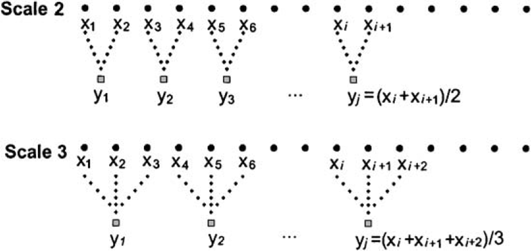
Schematic illustration of the coarse-graining procedure for scales 2 and 3.

SampEn quantifies the regularity of a time series. It reflects the conditional probability that two sequences of m consecutive data points which are similar to each other will remain similar when one more consecutive point is included. Being “similar” means that the value of a specific measure of distance is less than r. Therefore, SampEn is a function of m and r parameters. For all cases presented here, m = 2 and r = 0.15. In general, Pincus suggested m = 2 and r = 0.2 for the analysis of heart rate data. Previous studies of physiologic time series analysis have used an r value between 0.1 and 0.25. The values we chose fall within this range. More importantly, empirically, we found that our results were not very dependent on the specific values of m or r.

We applied MSE to the study of the stride interval times series derived from 10 young, healthy men (ages 18–29 yrs). The stride interval is a measure of the gait rhythm and is typically defined as the time interval between consecutive heel strikes of the same foot. To measure the stride interval, the output of ultra-thin, force sensitive switches was recorded on an ambulatory recorder and heel strike timing was automatically determined [12]. Subjects walked continuously on level ground for 1 h at their self-determined usual, slow and fast paces around an obstacle free outdoor track (Fig. 2).

Fig. 2.

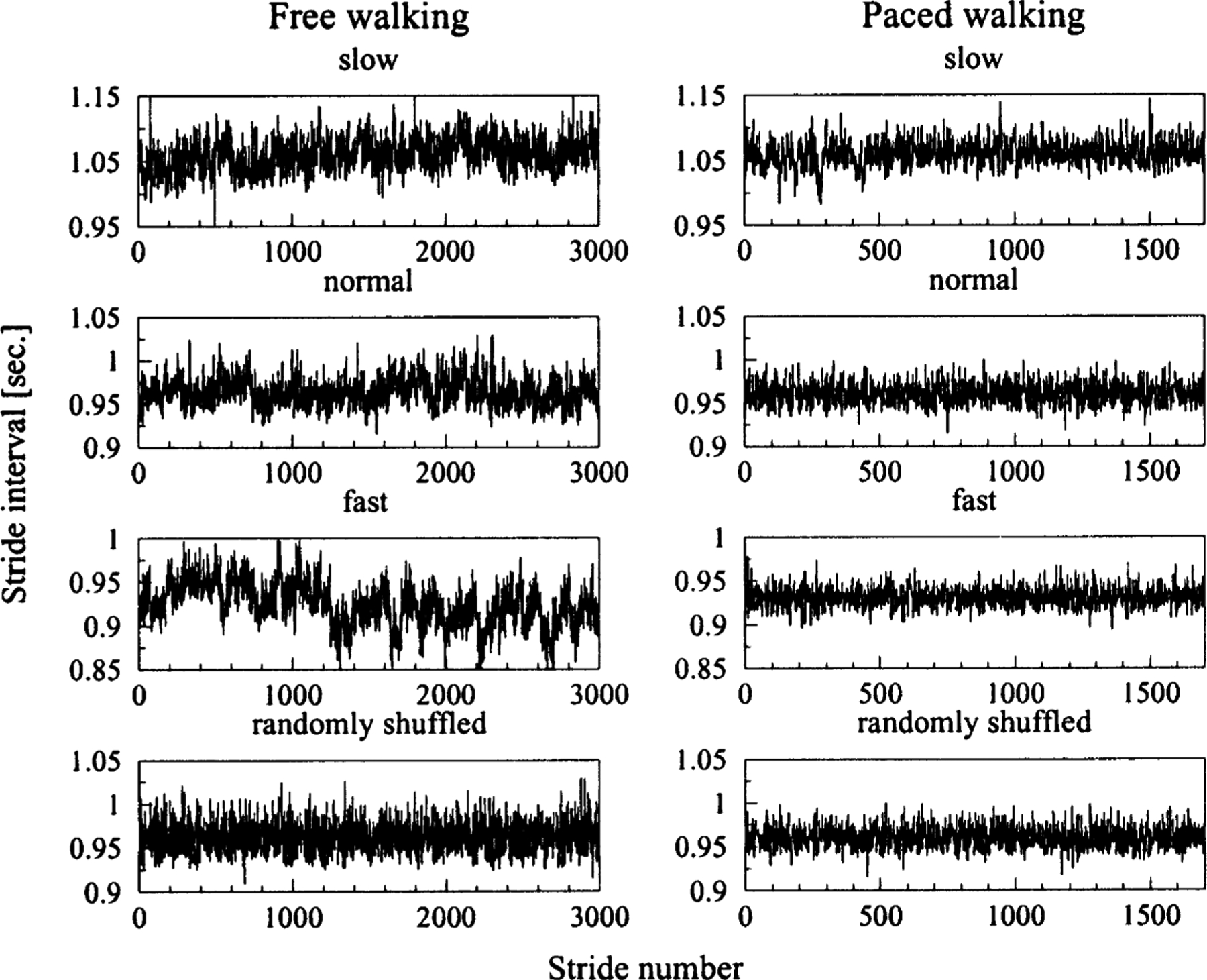
Representative stride interval time series obtained from a healthy subject who walked freely and in time to a metronome at slow, normal (usual) and fast rates. The last two time series are examples of randomized surrogate time series. They were generated by shuffling the values of the normal walking rate time series presented here.

In order to get further insight into the control mechanisms of human gait, the subjects were also asked to walk in time to a metronome that was set to each subject’s mean stride interval, computed from each of the three unconstrained walks (Fig. 2).

3. Results and discussion

We first applied the MSE method to compare the complexity of white and 1/f noise “control datasets”, i.e., uncorrelated and correlated fluctuations. Numerical simulations and analytic solutions are shown in Fig. 3a. The entropy for white noise time series monotonically decreases with the scale factor while the entropy for 1/f noise remains constant for all scales. Therefore, although for small scales white noise time series are assigned higher entropy values than 1/f noise time series, the opposite is true for scales larger than 5. These results are consistent with the fact that 1/f noise has structure on multiple scales and, therefore, is more complex than white noise.

Fig. 3.

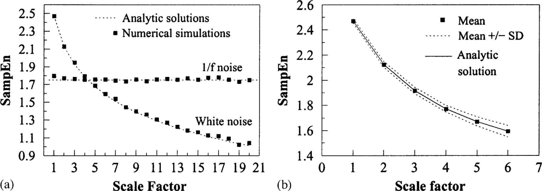
(a) MSE analysis of Gaussian distributed white noise (mean zero, variance one) and 1/f noise. On the y-axis, the value of SampEn [4] for the coarse-grained time series is plotted. Original time series have 3 × 10⁴ data points. The value of parameters m and r, defined in Ref. [7] are 2 and 0.15, respectively. The scale factor specifies the number of data points averaged to obtain each element of the coarse-grained time series. Symbols represent results of simulations and dotted lines represent analytic results. SampEn for coarse-grained white noise time series is analytically calculated by the expression: $-\text{ ln}{\int }_{-\infty }^{+\infty }\frac{1}{2}\sqrt{(\tau /2\pi )}[\text{erf}((x+r)/\sqrt{(2/\tau )})-\text{erf}((x-r)/\sqrt{(2/\tau )})]{\text{e}}^{-(1/2)x^2\tau }\text{ d}x$ (for any m ⩾ 1). τ and erf refer to the scale factor and to the error function, respectively. For 1/f noise time series, the analytic value of SampEn is a constant. Adapted from Ref [3]. (b) MSE analysis of a Guassian distributed white noise time series and 20 corresponding shuffled time series. The symbols refer to mean values of sample entropy (SampEn) for all time series and the broken lines to mean values ±SD. MSE curves for all time series should coincide with the analytic solution obtained for uncorrelated random noise. This is the case for scale one; but for larger scales, the dispersion of values around the analytic solution progressively increases due to the shortening of the length of the coarse-grained time series. To quantify these finite size effects, we calculated the area between the upper and lower curves, δ = 0.36. Two MSE curves were then considered significantly different if the area between them was > δ.

SampEn is largely independent of the time series length when the total number of data points is larger than approximately 750 [6]. For smaller time series, error bars due to finite size effects grow very fast as the total number of data points is reduced. Since the length of coarse-grained time series depends on the scale factor, the magnitude of the error bar for each SampEn value of the MSE curves also depends on the scale factor. To quantify this source of error, we considered a white noise time series and 20 surrogate data time series obtained by random shuffling of the original data point sequences. We calculated the MSE curves for all 20 surrogate time series and then, for each scale, we calculated the mean value of entropy ±SD (Fig. 3b). Next, we measured the area between the lower (mean value −SD) and the upper (mean value +SD) curves and used this value, (6), to determine whether two MSE curves were significantly different: MSE curves such that the area between them is ⩽ δ were considered not significantly different.

We next applied the MSE method to the analysis of the stride interval time series derived from subjects who walked freely at different speeds (Fig. 2). Previous studies, using detrended fluctuation analysis (DFA) [11,13] indicated that fluctuations of human gait cycle under free walking conditions do not represent uncorrelated random noise but, instead, exhibit long-range correlations with a power-law decay. This means that, at least in statistical terms, the value of any stride interval depends not only on the values of the most recent stride intervals but also on the values of those at relatively remote times (“memory effect”). These findings are indicative of very complex dynamics. We used the MSE method to quantify the complexity of the stride interval time series obtained from unconstrained walking at slow, normal and fast rates. We further tested the hypothesis that the complexity of these time series is encoded in the sequential ordering of the stride intervals and does not result from stride interval histograms. Therefore, for each physiologic time series, we built a surrogate time series by shuffling (randomly reordering) the sequence of data points. In this way, we destroyed correlations among the stride intervals while preserving the statistical properties of the distribution, particularly, the first and second moments.

In Fig. 4, the MSE results for unconstrained walking time series and their corresponding snuffled time series are presented. The curves shown are not the MSE curves for some particular time series but represent lines connecting the mean values of SampEn for all physiologic and surrogate time series. Of note, for scale 1, corresponding to traditional (single scale) SampEn, physiologic time series are assigned the lowest values of entropy. However, while the entropy for shuffled time series monotonically decreases with increasing scale factor, similar to white noise, the entropy for physiologic time series tends to stabilize between scales 2 and 4 for normal walking speed, and between scales 3 and 5 for slower and faster walking speeds. Therefore, for larger scales, the entropy for all unconstrained walking time series is larger than the entropy for the corresponding shuffled time series. The δ-values measuring the areas between original and surrogate time series for slow, normal and fast walking rates are 1.18, 0.68 and 0.89, respectively. These results show that physiologic time series are more complex than surrogate ones. Therefore, a model based on random fluctuations super-imposed on a constant value representing the mean walking speed does not account for all properties of the physiologic dynamical process. In addition, the results show (Fig. 4d) that during usual gait, normal free walking has the most complex dynamics followed by fast walking and finally slow walking. We note that the shuffled data in Figs. 4 and 5 are highly reproducible. Notice that these values are approximately the same as those presented in Fig. 3 corresponding to uncorrelated noise. Furthermore, Fig. 3 shows both analytic and numerical results of MSE for correlated and uncorrelated noise. Both agree and are quite robust.

Fig. 4.

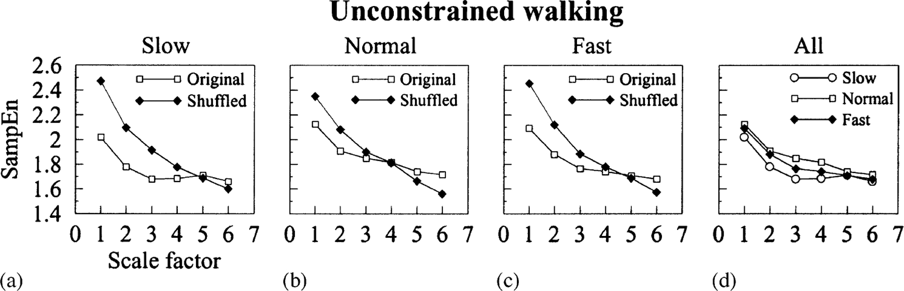
(a-d) MSE analysis of unconstrained walking time series derived from healthy subjects who walked for 1 h at slow, normal and fast rates (original time series), and of the corresponding surrogate shuffled time series. Curves represent lines connecting mean values of sample entropy (SampEn). The differences between mean MSE curves for physiologic and surrogate time series are all statistically significant. In all cases, physiologic time series are assigned higher entropy values than surrogate time series at larger scales. These results indicate that physiologic time series are more complex than surrogate ones. In addition, panel(d) shows that normal free walking dynamics are more complex than fast free walking dynamics, which in turn are more complex than slow free walking.

Fig. 5.

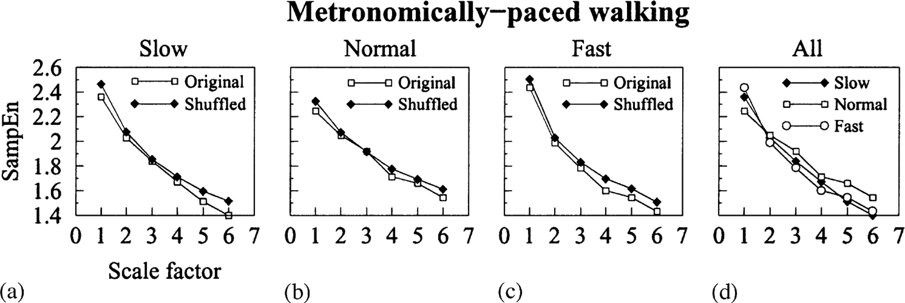
(a-d) MSE analysis of metronomically paced walking time series obtained from healthy subjects who walked at slow, normal and fast rates for 30 min, and of the corresponding surrogate time series. There is no qualitative difference between MSE curves corresponding to physiologic and surrogate time series. In all cases, the values of entropy monotonically decrease with the scale factor similar to white noise time series (Fig. 3), which indicates that all time series share a common random underlying dynamics.

In Fig. 5, we present the MSE results for metronomically-paced walking time series and their corresponding surrogate time series. Once again, the curves connect mean values of SampEn for all physiologic and surrogate time series. In contrast to the findings for spontaneous walking, there is no qualitative difference between MSE curves corresponding to physiologic and surrogate time series for all the paced walking speeds. MSE curves monotonically decrease with scale factor similar to the MSE curve of white noise time series (Fig. 3a). We measured the areas between physiologic and surrogate MSE curves for the three walking speeds. For normal paced walking time series, the area between the two MSE curves was 0.28, which is below the established level of statistical significance, 0.36 (Fig. 3 caption). Therefore, we concluded that they were not significantly different. For slow and fast paced walking time series, the areas between MSE curves were 0.41 and 0.40, respectively. These values are slightly larger than that corresponding to normal speed, but still very close to the minimum value of statistical significance. These results indicate that, in the case of paced walking, both physiologic and surrogate time series share a common random underlying dynamics. Since walking in time to a metronome has the effect of constraining supra-spinal pacesetters, these results indicate that control mechanisms above the level of the spinal cord are essential for the complex structure of free walking stride interval time series.

Finally, we note that our findings complement those obtained from previously reported DFA analysis of human gait data [10,13]. DFA revealed the presence of long-range correlations in free walking stride interval time series and their breakdown with metronomically-paced walking. To quantify the relationship between these two measures, we compared the results of MSE for scale 4 with the DFA results for the three different walking rates under free (non-metronomic) conditions. The correlation coefficients were lower than 0.46, indicating that the two methods, MSE and DFA, are not closely related.

In summary, we find that the spontaneous output of the human locomotor system during usual walking is more complex than walking under slow, fast or metronomically-paced protocols. The results obtained using the MSE technique are notable because they probe a dynamical property not identified by other statistics and have implications for quantifying and modeling gait control under physiologic and pathologic conditions.

References

- [1].Cover TM, Thomas JA, Elements of Information Theory, Wiley, USA, 1991. [Google Scholar]
- [2].Bar-Yam Y, Dynamics of Complex Systems, Addison-Wesley, USA, 1997. [Google Scholar]
- [3].Costa M, Goldberger AL, Peng C-K, Phys. Rev. Lett 89 (2002) 068 102. [DOI] [PubMed] [Google Scholar]
- [4].Zhang Y-C, Phys J. I France 1 (1991) 971. [Google Scholar]
- [5].Fogedby HC, J. Statist. Phys 69 (1992) 411. [Google Scholar]
- [6].Richman JS, Moorman JR, Am. J. Physiol 278 (2000) H2039. [DOI] [PubMed] [Google Scholar]
- [7].Pincus SM, Proc. Natl. Acad. Sci. USA 88 (1991) 2297. [DOI] [PMC free article] [PubMed] [Google Scholar]
- [8].Pincus SM, Ann. N. Y. Acad. Sci 954 (2001) 245, and references therein. [DOI] [PubMed] [Google Scholar]
- [9].Data available at /physiobank/database/#gait.
- [10].Hausdorff JM, Ashkenazy Y, Peng C-K, Ivanov PC, Stanley HE, Goldberger AL, Phys. A 302 (2001) 138. [DOI] [PubMed] [Google Scholar]
- [11].Hausdorff JM, Purdon PL, Peng C-K, Ladin Z, Wei JY, Goldberger AL, J. Appl. Physiol 80 (1996) 1448. [DOI] [PubMed] [Google Scholar]
- [12].Hausdorff JM, Ladin Z, Wei JY, J. Biomech 28 (1995) 347. [DOI] [PubMed] [Google Scholar]
- [13].Peng C-K, Hausdorff J, Goldberger AL, Fractal mechanisms in neuronal control: human hearbeat and gait dynamics in health and disease, in: Walleczek J (Ed.), Self-Organized Biological Dynamics and Nonlinear Control, Cambridge University Press, Cambridge, 2000, pp. 66–96. [Google Scholar]