

Abstract
We show that tax-induced increases in alcohol prices can lead to substantial substitution and avoidance behavior that limits reductions in alcohol consumption. Causal estimates are derived from a natural experiment in Illinois where spirits and wine taxes were raised sharply and unexpectedly in 2009. Beer taxes were increased by only a trivial amount. We construct representative and consistent measures of alcohol prices and sales from scanner data collected for hundreds of products in thousands of stores across the US. Using several difference-in-differences models, we show that alcohol excise taxes are instantly over-shifted. That is, a $1 tax increase translates into a price increase of up to $1.50. We find evidence suggesting that consumers react by switching to less expensive products. In particular, they increase purchases of beer, thus significantly moderating any tax-induced reductions in total ethanol consumption. Our study highlights the importance of tax-induced substitution, the implications of differential tax increases by beverage group and the impacts on public health of alternative types of tax hikes whose main aims are to increase revenue.
1. Introduction
Alcohol taxes are thought to be a valuable tool to reduce heavy alcohol consumption. Alcohol tax rates are based on three product groupings: spirits, wine and beer. Each group has its own excise tax rate and when alcohol excise taxes are increased it inevitably is done in a way that changes relative alcohol prices. The three classes of alcohol are to some degree substitutable and differential tax increases create substitutions that reduce the decline in overall alcohol consumption. We show that even though taxes are over-shifted to consumers, these substitutions can have a far greater impact on changes in total alcohol consumption than was understood in the past. Indeed, the data used in prior studies of this subject were generally too imprecise to measure induced substitutions. This paper combines a quasi-experimental design with high-resolution retail scanner data to investigate substitution patterns within and across different types of alcoholic products and to estimate the pass-through of alcohol taxes.
Most economic models predict that higher alcohol taxes, on either the producers, sellers, or consumers of alcohol, will translate into higher prices. Decades of research on the price elasticity of alcohol demand, in turn, have shown a negative correlation between alcohol prices and consumption. A recent meta-study by Wagenaar et al. (2009) found that the average elasticity estimates of this extensive literature are −0.46 for beer, −0.69 for wine, and −0.80 for spirits. However, past studies are subject to two major concerns. First, they use arguably unreliable price measures, often from a limited sample of stores and products, which have been shown to be prone to overstating elasticities and thus the effectiveness of alcohol taxes in reducing consumption (Ruhm et al., 2012). Second, previous research used observational study designs, such as interrupted time series or simple panel models, which may well suffer from endogeneity issues.
This paper overcomes these issues. We leverage detailed retail scanner data on alcohol sales in thousands of stores across the US to construct price measures that are based on a representative product basket and are consistent over time. We obtain credibly causal effects from these novel data by exploiting a natural experiment in Illinois where spirits and wine taxes were raised sharply and unexpectedly in 2009. We deploy classic difference-in-difference designs, event-study specifications, and the synthetic control method to estimate the effects of alcohol taxes on alcohol prices and sales. Moreover, our data allow us to shed light on cross-product-category substitution as well as substitution along the price distribution within product categories.
Our analysis suggests that consumers engage in cross-product substitution towards products that are subject to lower taxes. The 2009 Illinois excise tax increase resulted in higher spirits and wine prices but no change in beer prices. This resulted in higher beer sales, which partially offset the reductions in wine and spirits sales, and in total ethanol sales. We also document heterogeneous responses within spirits and wine categories. When products are defined in an inclusive fashion, sales of expensive ones show a smaller drop in sales than those of cheap brands. But when spirits products are limited to the 204 leading brands, which account for 55% of all sales and reflects the product basket available to consumers in a representative store, sales of bottom priced spirits increased by about 4%, while those of mid-tier products fell by 2%. Our study thus highlights the importance of substitutions induced by changes in relative tax rates. We also find that alcohol taxes are over-shifted by a factor of about 1.5. That is, a $1 increase in alcohol excise taxes on average translates into a price increase of up to $1.50. We illustrate that price increases tend to occur in $1 increments and that the pass-through does not vary very much at different points in the price distribution for spirits. For wine, over-shifting occurs primarily outside the top three deciles and is fully passed on for the most expensive wines.
This paper proceeds as follows. Section 2 summarizes the previous body of research on the effects of alcohol taxes with a focus on the data and methods used in these studies. It also introduces the natural experiment that we will exploit in this paper. Section 3 describes our main data and outlines the construction of our price and sales measures. In Section 4, we introduce our methodology. Section 5 presents the results, which are subjected to a series of robustness tests. We place our findings in the context of recent complementary studies of alcohol taxes in Section 6 before concluding in Section 7.
2. Background
2.1. Past Research
According to the National Institute on Alcohol Abuse and Alcoholism (2020), the economic cost of alcohol abuse in the United States was around $249 billion in 2010. These costs include over 88,000 deaths per year making alcohol the fourth leading cause of preventable mortality in the United States. Alcohol is also a major risk factor for various morbidities including heart disease and various forms of cancer and plays a significant role in traffic accidents (Saffer, 1997; Dee, 1999), crime (Carpenter, 2007), poor birth outcomes (Nilsson, 2017), risky sexual behavior (Markowitz et al., 2005), and unemployment (Cook and Moore, 2002). These direct and indirect costs have made the control of alcohol misuse a public health policy priority, especially since most of the costs of alcohol overuse and misuse are borne by the government and by individuals who do not abuse alcohol.
Government policy has often emphasized regulation over taxation of alcohol as means of addressing the external costs of alcohol abuse (for example, Grossman, 2017). Anti-drinking campaigns, for instance, have focused on the enactment of minimum legal drinking ages for the purchase and consumption of alcoholic beverages, the requirement that warning labels be placed on bottles and cans containing alcohol, and laws that call for stiff fines and penalties and that raise the probability of apprehension and conviction for the offense of driving under the influence of alcohol. Nevertheless, alcohol excise tax hikes, which have and continue to be used to raise revenue, are potential tools in this campaign.
Taxes affect both moderate consumers as well as heavy drinkers. Some prior studies show that the health costs of alcohol consumption are related to heavy consumption. For example, O’Keefe et al. (2018) argue that light or moderate alcohol consumption is associated with a lower risk for all-cause mortality, coronary artery disease, type 2 diabetes mellitus, heart failure, and stroke. In this case, alcohol taxes penalize moderate drinkers for the damage caused by heavy drinkers. This view has been challenged by Griswold et al. (2018) who argue that all-cause mortality, and cancer mortality specifically, rises with increasing levels of consumption and thus even moderate alcohol consumption is problematic. Others argue that policy-induced changes in average consumption reflect similar changes in heavy consumption (Smith, 1981).
The effect of a tax-induced price increase on alcohol consumption depends on the pass-through and the elasticity of demand. The pass-through is the ratio of the price increase to the tax increase. A textbook Cournot oligopoly model (Scherer and Ross, 1990) predicts that high industry concentration and low price elasticities will result in over-shifting taxes to consumers.1 Yet, there has been little past research on alcohol tax pass-throughs. One of the few studies that investigated this issue in the case of Alaska is Kenkel (2005), who found an alcohol tax pass-through greater than one. Shrestha and Markowitz (2016) confirm this result in the case of beer tax increases at the state and federal levels in the United States.
In contrast, there is an extensive literature on empirical estimates of alcohol price elasticities. Reviews by Gallet (2007) and Wagenaar et al. (2009) examined 132 and 112 past studies, respectively. Many of these studies struggle to find good measures of alcohol prices or sales. Most of the US literature (e.g., Manning et al., 1995; Grossman et al., 1998) has used alcohol prices provided by the American Chamber of Commerce Research Association (ACCRA). ACCRA collects these data in order to calculate a general Cost of Living Index for major US cities. Alcohol is only a small component of overall cost of living, which is why ACCRA only obtains the prices of a single brand of beer, wine, and whiskey in each city.2 Ruhm et al. (2012) show that these data are likely to suffer from measurement error, are unlikely to reflect the purchases of typical drinkers, and can severely and unpredictably bias estimates of alcohol demand elasticities. These factors suggest that it might be misleading to use existing price elasticities to predict the effects of recent tax hikes.
There are also difficulties in measuring alcohol consumption. Researchers have usually turned to survey data, such as the Behavioral Risk Factor Surveillance Survey (BRFSS) (Ruhm and Black, 2002), the National Epidemiologic Survey on Alcohol and Related Conditions (NESARC) (Nelson, 2013), or the Panel Study of Income Dynamics (PSID) and the Health and Retirement Study (HRS) (Dave and Saffer, 2008). Survey data, of course, may suffer from social desirability bias. For adolescents in particular, the direction of this bias is hard to determine. Moreover, these data usually only offer a crude consumption measure that also relies on respondents’ ability to retrospectively recall their drinking behavior. For instance, the number of drinks consumed in the past month is a popular measure of alcohol consumption in most surveys.
Finally, previous research typically relied on non-experimental research designs, such as interrupted time-series approaches or panel methods. For example, An and Sturm (2011) merge BRFSS data from different waves with state-level information on alcohol taxes in a given wave and use the resulting panel to correlate taxes with consumption. Indeed, using state tax rates as a proxy for alcohol prices – and thus avoiding the potential pitfalls of using ACCRA information – is a widespread practice, even though Young and Bielińska-Kwapisz (2002) have warned that alcohol taxes are not a good proxy for alcohol prices. Regardless of the price measure, the identifying variation in these setups often comes from inflation rather than changes in nominal prices or taxes. In addition, prices and taxes may be endogenously determined. Observational studies, therefore, might reflect spurious correlations between alcohol prices and consumption, even after including state and/or time fixed effects.
2.2. The Illinois Tax Increase
In this study, we exploit an unexpected, very substantial, and rapidly introduced excise tax increase in Illinois in 2009, to obtain causal estimates of alcohol tax pass-throughs and various changes in sales. The tax increase was included in the legislation of the “Illinois Jobs Now Act”. The legislation was a $31 billion state-construction plan focused primarily on construction of transportation infrastructure, but also had funding earmarked for school construction and community developments. The bill was passed rapidly within 10 weeks of a new governor taking office and went into effect on September 1, 2009.
While most of the state-construction plan was funded by issuing bonds, the bill also included a few measures designed to raise tax revenue, among them tax increases that were thought to raise $162 million from sales of candy, coffee, hygiene products, and alcohol (Center on Budget and Policy Priorities, 2010). Crucially, these alcohol tax increases were not instituted because of public health concerns or changing anti-alcohol sentiment in Illinois. The spirits excise tax was almost doubled from $4.50 to $8.55 per gallon, the wine tax also was almost doubled from $0.73 to $1.39 per gallon, and the beer taxes had a negligible increase of 4 cents per gallon. All taxes are assessed at the manufacturer level and paid by the distributor. Sales taxes were not affected.
The magnitude of the spirits excise tax increase is unprecedented. By way of comparison, the second largest spirits tax increase since 2006 (when our scanner data first became available) took place in Rhode Island in 2013 where the spirits excise tax increased from $3.75 to $5.40.3 The size of the Illinois tax increases, thus, allows for price and sales responses that are large enough to be detectable with our data, which we describe in the next section.
3. Data
A key innovation of this study is that price and sales measures are constructed from a wide range of stores and products. These data are derived from the NielsenIQ Retail Scanner data. Nielsen collects weekly point-of-sale data on revenue and volumes of about 2.6 million distinct products in over 35,000 stores. Products are identified by uniform product codes (UPC). There are several thousand distinct spirits and wine products. Most stores in the sample are grocery or drug stores, but Nielsen also obtains data from large mass merchandise stores and smaller liquor and convenience stores. The data are gathered in 52 markets and cover about 50% of the total sales volume in US grocery and drug stores.
Individual product prices (in $ per gallon) within a store are calculated by dividing total consumer spent per UPC by total gallon sales. To construct aggregate alcohol price measures that are representative for their product category but also consistent across time and different stores, we calculate our spirits price measure from a subset of more than 15,000 distinct spirits products, around 6,000 of which are on sale across the US in a given week. First, we exclude any transactions that relate to the “cocktails and coolers” product category and any products that are less than 60 proof (<30% alcohol). Second, only products in the most common bottle sizes (375ml, 750ml, 1000ml, and 1750ml) are used. The vast majority of excluded transactions comes from 50ml mini-sampler bottles. We also treat products that are essentially identical but have different UPCs as the same product. For example, holiday versions of a particular liquor type are not treated as distinct from the regular version. This also includes aggregating products that come in plastic and glass bottles. However, products of the same brand but with different container size are treated as distinct products. Third, very niche products are eliminated by including only products in our price index that had at least 10 transactions per day in at least one store. We also limit ourselves to products that were present in at least 18 of the 21 states that allow grocery store sales of spirits in the week of the tax change, and were being sold 2 years prior to the tax change and were still on the shelves two years after the tax change.
These exclusion criteria result in a product mix that consists of 204 products. Appendix Table A1 compares the characteristics of this product basket with the full market captured by the retail data. Our product basket accounts for about half of total sales within our balanced store sample. By definition, these are all top-selling products that have been available across the United States both before and after the Illinois tax reform. This consistency over time and location is crucial as selective changes in the availability of products might induce bias into our difference-in-differences estimator. Of course, there is a trade-off between consistency and representativeness. After all, one motivation for constructing this price index in the first place was the narrow focus of ACCRA price data on just a single product.
For each product, we calculate the price per gallon, so that we can construct a product price for each store in each week by dividing the total revenue created by a product by the number of gallons sold.4 A single store-week spirits price is then constructed as the unweighted, simple average of all 204 products. As a robustness check we also run our analysis using a sales-weighted price measure and conduct part of our analysis using all products available in Illinois and at least one control state (see details in Section 4).
Wine prices are constructed in the same manner: we exclude wine-flavored refreshments and alcohol-free wine; focus on bottle sizes of 187ml, 750ml, 1500ml, 3000ml, 4000ml, and 5000ml; unify virtually identical products; and only keep products that were present throughout our period of observation in at least 32 of the 35 states that allow wine sales in grocery stores, and that sold at least 80,000 units between September 2007 and August 2011. This results in a store-week wine price that is based on 252 distinct wine products, which account for about 50 percent of overall sales volume.
The main unit of observation in these data is the store-week. Stores in states that ban sales in grocery stores are dropped. To avoid issues related to selective attrition, we only use stores that are observed in every single one of the 210 weeks between the beginning of Sept. 2007 and the end of August 2011. For spirits, that leaves us with a balanced panel of 4,304 stores spread across the US. Three hundred twenty-seven of these stores are located in our treatment state, Illinois. Appendix Figure A1 shows the geographic distribution of these stores.5 Appendix Figure A2 illustrates the geographic distribution of the 9,356 stores in our balanced sample that sell wine. Both maps indicate that Nielsen stores are primarily sampled in urban areas. This is confirmed in Appendix Figures A3 and A4, which show that the majority of stores in Illinois is concentrated in the Chicago metropolitan area. It is important to note that – unlike other retail scanner data sets – our data are based on individual stores rather than retail market area aggregates.
Panel A of Table 1 provides an overview of our spirits price measures. The average price per gallon of spirits is around $80 in both Illinois and our control states in the two years prior to the tax change. This is equivalent to about $16 per 750ml bottle. In the post-period, the spirits price is markedly higher in Illinois. The raw data indicate that the difference between the change in price in Illinois in the post-period compared to the pre-period and the corresponding change in price in the control state amounts to $6.21 per gallon. This suggests that the tax hike of $4.05 per gallon was over-shifted. For each store-week in our sample, we also calculate aggregate spirits, wine, and beer sales in gallons based on all products sold in a given store during a given week rather than just those products in our basket that are used to calculate prices.6 In an average week, around 145 gallons of spirits are sold in a typical store in Illinois (162 in our control states). After the tax increase, sales per week in Illinois, relative to those in our control states, decline by 2.54 gallons or by about 2% of the pre-treatment mean in that state.
Table 1:
Descriptive Statistics - Table of Means
| Pre-treatment | Post-treatment | |||||
|---|---|---|---|---|---|---|
| Panel A: Spirits Outcome Measures | ||||||
| Control | Illinois | Difference | Control | Illinois | Difference | |
| Gallon-Price (in $) | 80.22 | 79.98 | 0.23 | 79.21 | 85.65 | −6.44 |
| Gallon Sales (per Store) | 161.58 | 144.94 | 16.64 | 165.70 | 146.51 | 19.18 |
| Panel B: Wine Outcome Measures | ||||||
| Control | Illinois | Difference | Control | Illinois | Difference | |
| Gallon-Price (in $) | 34.44 | 35.85 | −1.41 | 34.75 | 37.02 | −2.27 |
| Gallon Sales (per Store) | 214.97 | 329.75 | −114.78 | 223.74 | 328.97 | −105.23 |
| Panel C: Beer and Total Ethanol Sales | ||||||
| Control | Illinois | Difference | Control | Illinois | Difference | |
| Gallon Sales (Beer) | 1121.00 | 1630.01 | −509.00 | 1091.43 | 1655.56 | −564.14 |
| Gallon Sales (Ethanol) | 152.43 | 184.59 | −32.16 | 153.48 | 186.13 | −32.65 |
| Panel D: Product Basket Characteristics | |||
|---|---|---|---|
| Top 204 Spirits Products: | Top 252 Wine Products: | ||
| Share 375ml | 9.80 | Share 187ml | 0.04 |
| Share 750ml | 64.22 | Share 750ml | 0.58 |
| Share 1750ml | 25.98 | Share 1500ml | 0.29 |
| Share Gin | 8.33 | Share 3000ml | 0.02 |
| Share Cordials | 9.80 | Share 4000ml | 0.02 |
| Share Bourbon (Blended) | 1.47 | Share 5000ml | 0.02 |
| Share Canadian Whiskey | 7.84 | Share Domestic | 0.71 |
| Share Tequila | 8.33 | Share Imported | 0.2 |
| Share Bourbon (Straight) | 9.80 | Share Kosher | 0.01 |
| Share Vodka | 25.98 | Share Sangria | 0.01 |
| Share Brandy/Cognac | 6.37 | Share Sparkling | 0.06 |
| Share <$45 (Low-End) | 15.69 | Share <$30 (Low-End) | 0.49 |
| Share >$95 (High-End) | 37.25 | Share >$50 (High-End) | 0.15 |
| Panel E: Store Characteristics | ||
|---|---|---|
| Spirits Stores | Wine Stores | |
| Share Grocery Stores | 67.33 | 65.22 |
| Share Drug Stores | 24.65 | 20.88 |
| Share Mass Market Stores | 2.32 | 9.09 |
| Share Liquor Stores | 4.21 | 1.93 |
| Share Convenience Stores | 1.49 | 2.88 |
Notes: The unit of observation in all measures in Panel A-C is the store-week. Pre-treatment refers to the two years before 1 September, post-treatment refers to the 2 years after. Panel D shows the characteristics of our product baskets that we base our price analysis on. Panel E shows the characteristics of the 4,304 and 9,356 stores in our sample that sell spirits and wine respectively.
Panel C presents total beer sales in gallons and total ethanol sales for each store-week, which we analyze in order to investigate substitution patterns.
Panel D of Table 1 provides additional information on the composition of our product basket that is used to calculate our spirits price. The basket is dominated by 750ml bottles and contains all kinds of different spirits with different varieties of whiskey (bourbon, scotch, etc.) and vodka making up the largest shares. Sixteen percent of products cost less than $45 per gallon (or $9 per 750ml) and 37 percent of products cost more than $95 per gallon. Overall, our product mix covers a diverse range of different spirit types and several price segments. Panel D shows that the vast majority of stores in our sample are grocery and drug stores, which reflects the fact that Nielsen cooperates with 90 major chains to collect the data.
Similar to spirits, the raw data of Panel B in Table 1 suggest that the wine excise tax increase was over-shifted. The tax increase was $0.66 per gallon, but prices in Illinois increased by $0.86 relative to prices in our control states. The raw data are also indicative of a negative sales response of about 3% relative to mean sales per week in Illinois in the pre-treatment period. Panel D shows that our sample of wine products is dominated by domestic wine in 750ml or 1500ml bottles. Almost 50% of products are sold at under $6 per 750ml (or $30 per gallon). Our representative wine price is thus, not constructed from fine wines but from widely available inexpensive products that are primarily sold in grocery and drug stores (see Panel E).
4. Methodology
4.1. Main Approach: Difference-in-Differences
The 4,304 stores across the US that sell spirits in all 210 weeks under consideration, give us a sample with 903,840 observations to analyze the effect of the tax change on spirits prices and sales; our balanced sample of 9,356 wine-selling stores provides 1,964,760 observations. Our unit of observation is the store-week, i.e., we have a representative price and sales for every store in every week. We combine these data with the quasi-experimental exogenous variation created by the Illinois tax increase through a difference-in-differences model, estimated using OLS, of the following form:
| (1) |
where ysjt is price or sales outcome in store s, located in state j, in week t, γs denotes a full set of store fixed effects. These time-invariant fixed effects subsume any state fixed effects. The vector θt is a set of week fixed effects common across stores, although in most specifications we use year-month fixed effects, which does not affect the results, but allows us to cleanly plot the results of an event-study-specification. Time fixed effects also subsume the post-treatment-period indicator of a classic difference-in-differences setup. Treatjt is an interaction between a dummy indicator for whether a store is located in Illinois (our treatment state) and a dummy indicator for whether an observation pertains to a week after September 1, 2009 (our post-period), and usjt is the disturbance term.
Our main coefficient of interest is βDD, which yields the treatment effect. That is the effect of the excise tax increase on prices and sales in Illinois relative to those in our control states where taxes were not raised.7 We also run several event-study specifications in which the single treatment indicator of equation (1) is replaced by a set of year-month dummies, interacted with a treatment state indicator:
| (2) |
The lags in the specification allow us to evaluate whether any effect of the tax increase grows over time or fades out. The leads provide an additional test of the main identifying assumption, which is that trends in our outcomes of interest would have continued to be the same in Illinois and the control states in the absence of the tax increase.
Panel A of Figure 1 provides a first piece of evidence for this “common time-trends assumption”. The thin solid line plots the mean per-gallon price in Illinois stores for the four-year period under evaluation. The figure plots raw, unweighted means. That is, every store carries the same weight. The figure reveals substantial seasonality, especially around the Christmas holidays. In order to not have the data obscured by this seasonality, we overlay the raw means with a thick solid Locally Weighted Scatterplot Smoothing (LOWESS) line. We repeat this procedure for stores in control states, which are shown in Figure 1 with dashed lines.
Figure 1: Trends in Spirits Prices and Sales.

Notes: These graphs display store-averages in spirits prices (in $) and gallon sales, aggregated to the treatment state (Illinois) and control state (all other states) levels. In these calculations, each store received the same weight. The thin lines display the raw data (no seasonal adjustments are made) and are overlaid with thicker Locally Weighted Scatterplot Smoothing (LOWESS) lines.
The data show that spirits prices in Illinois and the control states are on strikingly similar trajectories prior to the tax increase. In fact, even the seasonal jump in prices around the holiday season is all but identical in Illinois and the control states. Second, spirits prices diverge sharply during the week in which the excise tax went up, indicated by the black dotted vertical line. This jump corresponds to about a $6 increase in price and the gap between Illinois and the control states persists until mid-2011. Not surprisingly, the size of this one-off shift in prices is also consistent with the over shifting result implied by our descriptive statistics in Table 1.
Panel B of Figure 1 plots raw and smoothed data for spirits sales. Similar to spirits prices, gallon-sales per store appear to follow identical pre-treatment time trends in Illinois and our control states. Both sets of stores are subject to the same seasonality, although the sales spike around Thanksgiving and Christmas may be slightly more pronounced in Illinois. We account for this pattern by seasonally adjusting our spirits sales data. Specifically, we regress gallon-sales on a set of calendar month dummies interacted with Illinois dummies to account for potentially differential seasonality. We then use the residuals in our main analysis. In practice, seasonal adjustment makes little difference and our main results using unadjusted data are reported in the Appendix.
In contrast to spirits prices, the raw data gives less of an indication that spirits sales may have changed. Of course, the scale and lack of controls may mask important features that are only uncovered by a more detailed regression analysis. There is, however, a small increase in Illinois sales in the week prior to the tax change. We address such anticipatory effects using a “donut” approach outlined below, although Figure 1 suggests that any bias induced by anticipatory behavior should be negligible.
Figure 2 shows trends in the raw data for wine prices and wine sales. Panel A documents that wine prices are slightly higher in Illinois than in our control states, but they follow very similar trends. There is a clear break at the time of the tax increase, such that the price gap widens by a magnitude that suggests over-shifting, albeit to a slightly smaller extent than observed for the spirits tax increase. Wine sales show slightly more extreme seasonal patterns around the Christmas and Thanksgiving periods.8 Again, we seasonally adjust the sales data and report the unadjusted results in the Appendix. The raw data also show no obvious divergence for wine sales, the gap between sales in Illinois stores and control stores appears to shrink only marginally.
Figure 2: Trends in Wine Prices and Sales.

Notes: These graphs display store-averages in wine prices (in $) and gallon sales, aggregated to the treatment state (Illinois) and control state (all other states) levels. In these calculations, each store received the same weight. The thin lines display the raw data (no seasonal adjustments are made) and are overlaid with thicker Locally Weighted Scatterplot Smoothing (LOWESS) lines.
Our sales analyses are always based on gallon-sales aggregations of all products. As a robustness check and for subgroup analyses, we also run both our sales and price analyses at the individual product level, using information on all products, which in a given week saw at least one transaction in both Illinois and one of our control states. For computational ease, we aggregate our data to treatment-control differences at the product-week level in these analyses:
| (3) |
where Δypct is the difference in outcome in week t for product p between Illinois and our control state aggregate. Postt is equal to one for weeks after 1 September 2009, and γp represents a full set of product fixed effects. Because the tax increase occurs in a single state at one point in time, this setup is equivalent to an analysis at the product-store-week level. Also note that this specification has outcome differences on the left-hand side. This implicitly controls for product-specific period effects. However, considering all products for this analysis results in a highly unbalanced panel that includes niche products that show up in both Illinois and a control state very sporadically. Our analysis for spirits is based on 3,256 spread across 259,196 product-week observations, and 5,837 wine products spread across 514,573 observations. This is nonetheless a useful robustness check and the fact that results from the models represented by equation (2) and (3), respectively, turn out to be very similar adds credibility to our estimates.
4.2. Alternative Standard Errors
The group structure in our data creates an issue for the calculation of valid standard errors. All of the stores in the same state might be subject to common influences creating a clustering problem. As is standard in the literature (Bertrand et al., 2004), we therefore cluster the standard errors at the state-level in our baseline specification.
A related issue is that while there are thousands of stores in our sample, we effectively only have one treatment group (stores in Illinois) and one control group (stores in other states). Therefore, we adopt the procedure by Donald and Lang (2007) to obtain appropriate standard errors in difference-in-differences (DD) models with only one large treatment group and one large control group observed over multiple before- and aftertreatment periods. In the first step of their two-step procedure, both treatment and control stores are collapsed into treatment and control averages. In the context of our study, this means that we go from 4,304 (stores) × 210 (weeks) to 2 × 210 observations. We can then calculate the difference in outcomes between our treatment state aggregate and the control state aggregate. In a second step, we regress this difference on an indicator for the post-treatment period that is equal to one for half of our 210 weekly observations, and zero for pre-treatment differences:
| (4) |
Because each store receives the same weight in the construction of our treatment and control aggregates, the Donald and Lang (2007) method ensures that βDL in equation (4) will be identical to βDD of equation (1) but calculates standard errors that reflect the difference in yt between the treatment and control groups in each of 210 periods. Throughout our results section we report both the regular cluster-adjusted standard errors as well as standard errors obtained using the above procedure, which we refer to as “Donald-Lang standard errors.” In addition, we re-run the pure time series regression given by equation (4) and calculate standard errors using the method of Newey and West (1987). These standard errors are auto-correlation consistent in that they allow for correlated shocks to the disturbance term (ut) to have persistence over 3 weeks.9
4.3. Anticipatory Effects and Adjusted Control Group
Figures 1 and 2 support our main identifying assumption. So does the event-study specification, which will be shown in Section 5. Nonetheless, one may be concerned that anticipatory effects may bias our estimates. In order to address any such concerns, we re-run all analyses excluding observations that pertain to either the “treatment week” (i.e., the week ending on Saturday, 5 September 2009), or the three weeks following the treatment week, or the four weeks preceding the treatment week. In other words, we reduce the number of observations per store from 210 to 202. The idea here is that any stocking up by consumers is likely to have occurred in the weeks leading up to the tax increase, and that this may have depressed sales in the weeks following the tax increase. Such behavior would bias our estimates away from zero, i.e., we might overestimate the extent to which the tax reduced sales. A “donut”-specification that cuts out the middle part of the time period we analyze addresses this issue and at the very least provides a useful robustness check.
One might still be concerned about whether all the stores in states outside of Illinois are a valid comparison group to those in Illinois. As an additional robustness check, we therefore use the “synthetic control” method developed by Abadie et al. (2010). This technique constructs a synthetic control group that approximates the outcome in the treatment group as closely as possible by selecting a weighted combination of untreated units. The control units are usually selected based on pre-treatment characteristics and pre-intervention outcome data, in our case only the latter. We describe the procedures we use to implement this method in the third section of the Appendix.
5. Results
Tables 2-5 follow the structure outlined above. Column (1) shows the coefficient for the conventional difference-in-differences regression outlined in equation (1). In this specification all control states serve as a comparison group. Column (2) repeats the analysis but discards data that refer to time periods either 4 weeks prior or after the tax change. In column (3) the control group is constructed using the synthetic control approach; column (4) combines the synthetic control method with our donut estimation. We report three sets of standard errors: State-cluster adjusted standard errors, standard errors calculated using Donald and Lang (2007) two step procedure (DL-standard errors), and DL models with Newey-West standard errors. Finally, in column (5) we we-run our analysis at the product-level as described by equation (3).
Table 2:
Regression Results –Spirits Prices
| (1) Main |
(2) Donut |
(3) Synth |
(4) Synth-Donut |
(5) Product-Level |
|
|---|---|---|---|---|---|
| Treatjt | 6.623*** | 6.717*** | 6.521*** | 6.635*** | 7.167*** |
| Cluster SEs | (0.438) | (0.451) | - | - | (0.270) |
| Donald-Lang SEs | (0.131) | (0.117) | (0.144) | (0.121) | - |
| DL - Newey - West SEs | (0.268) | (0.181) | (0.239) | (0.201) | - |
| Observations | 903,840 | 869,408 | 210 | 202 | 259,196 |
| R-squared | 0.788 | 0.787 | 0.908 | 0.938 | 0.490 |
| Store-Fixed-Effects | Yes | Yes | No | No | n.a. |
| Year-Month-Fixed-Effects | Yes | Yes | No | No | n.a. |
| Seasonal Adj. | Yes | Yes | Yes | Yes | Yes |
Notes: In column (1), the dependent variable is the average spirits price in the store-week cell. Treatjt equals one for Illinois (treatment) stores from Sep 2009 on, and zero otherwise. Cluster SEs refer to clustering at the state level for column (1) and product level for column (5). Donald-Lang and DL-Newey-West: The dependent variable is the difference in the Illinois and the control states’ store-average, by week. Sample size is 210 weeks. Newey-West method adjusts for first-order autocorrelation with maximum lag set at 3 weeks. Donut-specifications leave out 8 weeks around policy change. In columns (3) and (4), the dependent variable is the difference between Illinois state aggregates and a synthetic control state aggregate. The results in column (5) corresponds to regression equation (3). Here the dependent variable is the difference in average spirits price between treatment and control aggregates at the product-week level. Treatjt here equals one for periods from Sep 2009 on, and zero otherwise.
indicate statistical significance at the 1%/5%/10%-level.
Table 5:
Regression Results – (Log) Wine Sales
| (1) Main |
(2) Donut |
(3) Synth |
(4) Synth-Donut |
(5) Product-Level |
|
|---|---|---|---|---|---|
| Treatjt | −0.030*** | −0.029*** | −0.042*** | −0.042*** | −0.048*** |
| Cluster SEs | (0.009) | (0.009) | - | - | (0.005) |
| Donald-Lang SEs | (0.006) | (0.006) | (0.004) | (0.004) | - |
| DL - Newey - West SEs | (0.006) | (0.006) | (0.005) | (0.005) | - |
| Observations | 1,964,760 | 1,889,912 | 210 | 202 | 514,573 |
| R-squared | 0.967 | 0.967 | 0.340 | 0.341 | 0.370 |
| Store-Fixed-Effects | Yes | Yes | No | No | n.a. |
| Year-Month-Fixed-Effects | Yes | Yes | No | No | n.a. |
| Seasonal Adj. | Yes | Yes | Yes | Yes | Yes |
Notes: In column (1), the dependent variable is the natural logarithm of total wine gallon sales in the store-week cell. Treatjt equals one for Illinois (treatment) stores from Sep 2009 on, and zero otherwise. Cluster SEs refer to clustering at the state level for column (1) and product level for column (5). Donald-Lang and DL-Newey-West: The dependent variable is the difference in the Illinois and the control states’ store-average, by week. Sample size is 210 weeks. Newey-West method adjusts for first-order autocorrelation with maximum lag set at 3 weeks. Donut-specifications leave out 8 weeks around policy change. In columns (3) and (4), the dependent variable is the difference between Illinois state aggregates and a synthetic control state aggregate. The results in column (5) corresponds to regression equation (3). Here the dependent variable is the difference in average wine (log) sales between treatment and control aggregates at the product-week level. Treatjt here equals one for periods from Sep 2009 on, and zero otherwise.
indicate statistical significance at the 1%/5%/10%-level.
5.1. Results for Spirits
Table 2 summarizes our results for the pass-through of the excise spirits tax increase. It is striking that all five specifications yield point estimates that are of very similar size and statistically significant at any reasonable level of significance. Column (1) suggests that the tax increase led to a spirits price increase of $6.62 per gallon. Since the excise tax increase was $4.05 per gallon, this indicates a pass-through of about 1.5. We can also reject the null hypothesis of a complete 1:1 pass-through at any reasonable significance level. In other words, the tax is over-shifted. In percentage terms, the almost 100 percent increase in the tax rate increased the price of spirits by approximately 8.2%.10
Panel A of Figure 3 illustrates the results of the event-study specification outlined by equation (2). The reference period here is the first week in our sample, i.e. the week ending on September 9, 2007. Two features stand out. First, the pre-period coefficients and 95% confidence intervals all hover around zero. This further bolsters the common-time trend assumption and thus adds credibility to a causal interpretation of our results. Second, prices appear to adjust almost immediately and remain at a higher level for the full 2-year post-period. This suggests that the tax increase led to over-shifting that resulted in a permanent price increase.
Figure 3: Event-Study Results - Spirits.
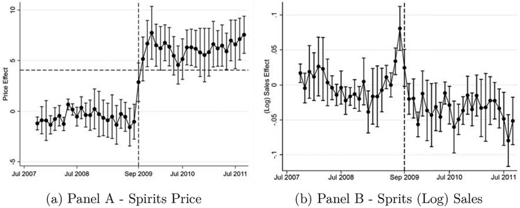
Notes: These figures show the results of the event-study specification as specified in equation (2). That is, each dot is the point estimate of a month-year fixed effect interacted with our treatment state indicator. Confidence intervals are adjusted for clustering at the state level. The reference period is September 2007. The dependent variables are spirits price and log spirits sales at the store-week level. The horizontal dashed line indicates full pass-through. The vertical dashed line indicates the date of tax change.
Our product-level analysis helps to further unpack the price response. First, column (5) of Table 2 shows that an analysis at the product level rather than store-price aggregates yields a very similar over-shifting result of $7.17 per gallon. This is equivalent to a pass-through of $1.85 per 750ml bottle, which is the most common container size on a tax increase of about $1.07. Previous work by Conlon and Rao (2020) suggests that retail alcohol prices often change in one dollar increments, which may contribute to tax over-shifting. Figure 5a confirms and illustrates this pattern. Here we focus on products in 750ml bottles in Illinois. For each product we calculate the modal price in the five weeks leading up to the tax change and five weeks after the tax change.11 It is striking that our over-shifting result appears to be driven by a combination of products whose price increased by either $1, $2, or another $1 increment. Of course, this is a mainly descriptive analysis (see Conlon and Rao, 2020, for a more detailed analysis based on more tax hikes that goes beyond the scope of our study), but it suggests that prices are, for the most part, either unchanged or increase incrementally, and that it is a combination of these two behaviors that generates our over-shifting results.
Figure 5: Price Shifts after Tax.

Notes: These figures show the change in the modal price for each product that had a transaction in an Illinois store in the five weeks before the tax change and the five weeks after the tax change. Sample is limited to 750ml bottles.
Table 3 shows the results for (log) spirits sales.12 Column (1) suggests that the tax increase resulted in about a 3.5 percent reduction in gallon sales. The effect is statistically significant at the 1% level regardless of how the standard errors are obtained. Picking the control group using the Abadie et al. (2010) method slightly increases the point estimate although there is no statistically significant difference across specifications. Our product-level analysis, on the other hand, yields a slightly smaller point estimate, but again we cannot reject the null hypothesis of no difference with our main estimate.
Table 3:
Regression Results – (Log) Spirit Sales
| (1) Main |
(2) Donut |
(3) Synth |
(4) Synth-Donut |
(5) Product-Level |
|
|---|---|---|---|---|---|
| Treatjt | −0.035*** | −0.033*** | −0.043*** | −0.042*** | −0.026*** |
| Cluster SEs | (0.008) | (0.009) | - | - | (0.006) |
| Donald-Lang SEs | (0.008) | (0.007) | (0.006) | (0.006) | - |
| DL - Newey - West SEs | (0.008) | (0.007) | (0.006) | (0.006) | - |
| Observations | 903,840 | 869,408 | 210 | 202 | 259,196 |
| R-squared | 0.951 | 0.950 | 0.193 | 0.210 | 0.460 |
| Store-Fixed-Effects | Yes | Yes | No | No | n.a. |
| Year-Month-Fixed-Effects | Yes | Yes | No | No | n.a. |
| Seasonal Adj. | Yes | Yes | Yes | Yes | Yes |
Notes: In column (1), the dependent variable is the natural logarithm of total spirits gallon sales in the store-week cell. Treatjt equals one for Illinois (treatment) stores from Sep 2009 on, and zero otherwise. Cluster SEs refer to clustering at the state level for column (1) and product level for column (5). Donald-Lang and DL-Newey-West: The dependent variable is the difference in the Illinois and the control states’ store-average, by week. Sample size is 210 weeks. Newey-West method adjusts for first-order autocorrelation with maximum lag set at 3 weeks. Donut-specifications leave out 8 weeks around policy change. In columns (3) and (4), the dependent variable is the difference between Illinois state aggregates and a synthetic control state aggregate. The results in column (5) corresponds to regression equation (3). Here the dependent variable is the difference in average spirits (log) sales between treatment and control aggregates at the product-week level. Treatjt here equals one for periods from Sep 2009 on, and zero otherwise.
indicate statistical significance at the 1%/5%/10%-level.
Panel B of Figure 3 shows the results of our event-study specification. Despite our seasonal adjustment, sales are much noisier than prices. Nonetheless, the lagged interaction coefficients hover around zero for the vast majority of the period leading up to September 2009. The graph also indicates that sales spiked in Illinois, relative to other states, in the month prior to the tax increase. We can see about a 10 percent increase in sales in the month prior to the tax increase. However, the donut-specification of columns (2) and (4) in Table 3 produces point estimates that are virtually identical to those that use the full time period. In other words, there is evidence for anticipation behavior, but it does not appear to play a large enough role to significantly affect our headline estimate. It is notable that from 2010 on, sales settle at a level that is markedly lower than prior to the tax increase. The event study estimates suggest a reduction of about 3 percent, which – not surprisingly – corresponds to the point estimates of Table 3. Naturally, our event-study estimates are less precisely estimated than the corresponding single-coefficient point estimates and the confidence intervals suggest that some of the lags are not statistically significantly different from zero at the 5% level. However, the overall pattern of the specification adds credibility to our headline estimate.
5.2. Results for Wine
We also evaluate the pass-through and sales-response for the 2009 increase in the Illinois wine tax, using the same difference-in-differences setup. Column (1) of Table 4 suggests that the wine-tax increase of $0.66 per gallon resulted in a price increase of $0.84 per gallon. The shift is statistically significant at any reasonable level of significance and stable across donut (column 2) and synthetic control specifications (columns 3 and 4) as well as alternative ways of calculating the standard error. The suggested pass-through of about 1.3 is slightly smaller than for spirits. We can again firmly reject the null-hypothesis of a complete 1:1 pass-through (p-value < 0.001). Clearly, the wine tax was also over-shifted to the consumer.13 In percentage terms, the almost 100 percent increase in the tax rate increased the price of wine by approximately 2.4%.14 The results of our event-study specification, shown in Panel A of Figure 4, are slightly noisier than the equivalent for spirits. They nonetheless support the common time-trend assumption and show a clear break at the time of the tax increase when wine prices shifted up abruptly.
Table 4:
Regression Results – Wine Prices
| (1) Main |
(2) Donut |
(3) Synth |
(4) Synth-Donut |
(5) Product-Level |
|
|---|---|---|---|---|---|
| Treatjt | 0.842*** | 0.856*** | 0.786*** | 0.799*** | 1.191*** |
| Cluster SEs | (0.145) | (0.149) | - | - | (0.125) |
| Donald-Lang SEs | (0.049) | (0.086) | (0.044) | (0.045) | - |
| DL - Newey - West SEs | (0.084) | (0.049) | (0.074) | (0.076) | - |
| Observations | 1,964,760 | 1,889,912 | 210 | 202 | 514,573 |
| R-squared | 0.814 | 0.813 | 0.602 | 0.607 | 0.370 |
| Store-Fixed-Effects | Yes | Yes | No | No | n.a. |
| Year-Month-Fixed-Effects | Yes | Yes | No | No | n.a. |
| Seasonal Adj. | Yes | Yes | Yes | Yes | Yes |
Notes: In column (1), the dependent variable is the average wine price in the store-week cell. Treatjt equals one for Illinois (treatment) stores from Sep 2009 on, and zero otherwise. Cluster SEs refer to clustering at the state level for column (1) and product level for column (5). Donald-Lang and DL-Newey-West: The dependent variable is the difference in the Illinois and the control states’ store-average, by week. Sample size is 210 weeks. Newey-West method adjusts for first-order autocorrelation with maximum lag set at 3 weeks. Donut-specifications leave out 8 weeks around policy change. In columns (3) and (4), the dependent variable is the difference between Illinois state aggregates and a synthetic control state aggregate. The results in column (5) corresponds to regression equation (3). Here the dependent variable is the difference in average wine price between treatment and control aggregates at the product-week level. Treatjt here equals one for periods from Sep 2009 on, and zero otherwise.
indicate statistical significance at the 1%/5%/10%-level.
Figure 4: Event-Study Results - Wine.

Notes: These figures show the results of the event-study specification as specified in equation (2). That is, each dot is the point estimate of a month-year fixed effect interacted with our treatment state indicator. Confidence intervals are adjusted for clustering at the state level. The reference period is September 2007. The dependent variables are wine price and log wine sales at the store-week level. The horizontal dashed line indicates full pass-through. The vertical dashed line indicates the date of tax change.
Similarly, Panel B of Figure 4 shows a clear break for wine sales at the time of the tax increase. All pre-treatment interaction terms hover around zero, but wine sales in Illinois decreased by 3-4 percent after the tax increase kicked in. This is consistent with the aggregate point estimate of Table 5. Columns (1) and (2) indicate that the tax increase led to a drop in wine sales of about 3%. Our synthetic control estimation, shown in column (3) indicates a slightly larger drop of 4.2%. All effects are statistically significant at the 1% level regardless of the how the standard errors are calculated.
It is again notable that a product-level analysis in the mold of regression equation (3) yields similar results for both our estimate of the wine-tax pass-through and the corresponding sales response (see column (5) of Tables 4 and 5, respectively). Similar to spirits, Figure 5b shows that the pass-through result is driven by a combination of $1 incremental price increases and products for which the price was not adjusted at all, indicating that for some products the tax increase is absorbed along the value chain.
5.3. Substitution across Price Segments
Our aggregate, store-level wine and spirits prices were based on a heterogeneous product basket. In this section, we focus our analysis to finer subgroups. In particular, we investigate whether the taxes were passed on uniformly across price segments. For instance, it is conceivable that price increases could be concentrated at the top end if consumers of cheap spirits were more price-conscious and retailers, therefore, raise prices less in this segment. In addition, consumers might react to price increases by substituting towards cheaper products within the same product category.
We turn to a product-level analysis to better understand within product category substitution patterns. Specifically, we split our products into price-decile,s which are defined based on average prices in the two years prior to the tax increase. We then re-run our product-week level analysis given by equation (3) for each of the ten price segments. The coefficients and 95% confidence intervals from this analysis are shown in Figure 6.
Figure 6: Price and Sales Response by Price Point.

Notes: These figures show estimates for the tax pass-through (in $) and (log) gallon sales by price point. Blue squares indicate the point estimates for spirits that are accompanied by 95% confidence intervals. Red circles show the same results for wine. The dashed line in Figure (a) indicate a price change that corresponds to a complete 1:1 pass-through. All estimates correspond to regression equation 3.
Sub-figure 6a shows our estimates of the pass-through separately for spirits (blue squares and confidence bands) and wine (red circles and confidence bands). Our analysis shows that for spirits, the pass-through was almost uniform across price segments. All point estimates are to the right of the blue dashed vertical line for a 1:1 pass-through, thus suggesting that the tax was overshifted in all price segments. For wine, our analysis suggests that the tax was also clearly over-shifted for lower price-deciles whereas for the three highest deciles we cannot reject the null hypothesis of a full pass-through at any reasonable level of significance.
For sales, on the other hand, there is substantial heterogeneity across price points. While the standard errors are naturally larger than for the full sample, the point estimates for spirits sales in sub-figure 6b hint at a sales response that was close to zero for expensive spirits but quite substantial for low-price spirits. For instance, the point estimate for the lowest decile suggests that sales of the cheapest spirits dropped by 7.2% whereas those in the top decile remained unchanged. We find a similar, arguably even more pronounced pattern for wine sales (red squares).15
There are several explanations for these heterogeneous effects. First, while the pass-through was uniform in absolute terms (for spirits), in percentage terms cheap products saw a larger relative price increase, which may well trigger a stronger demand response. Second, consumers of inexpensive wine and spirits might be more price sensitive than those of fine wines and expensive spirits. Third, it is conceivable that retailers react to the tax by introducing more low-price products to their shelves. However, an analysis of product entry/exit patterns reveals that products which started to appear in our data only after the tax increase, account for less than 1% of total sales volume and these tend, in fact, to be pricier than existing products. Finally, it is also possible that our estimates mask a cascade of substitutions where some consumers of mid-priced spirits and wines switch to slightly cheaper alternatives with some of those consuming the cheapest products ceasing to consume as there is no cheap substitute available. This cascading then partially offsets some of the sales reductions in certain price categories that otherwise would be observed.
While it is beyond the scope of this paper to fully disentangle the exact mechanism and it is likely that a combination of effects is at play, a complementary analysis of our main product basket hints at within category substitution. This is shown by Appendix Table A12, which limits spirits products to the 204 leading brands that account for 55% of all sales and reflect the product basket available to consumers in a representative store. We split this product basket into the 51 least expensive, 102 mid-tier and 51 most expensive products (based on pre-treatment prices). Column (4) of Panel A suggests that gallon sales of bottom priced spirits increased by about 4.1%. Sales of mid-tier products dropped by 1.9% and expensive spirits products were unaffected. Because our spirits sample in this analysis is slightly biased away from very cheap liquor, this substitution pattern is consistent with consumer down-grading across the price distribution (except for the very top of the price distribution). Columns (4) to (6) of Panel B are also consistent with such consumer behavior as it shows that for the most popular wine products - a sample that is skewed towards cheaper wines - the largest sales drops are concentrated in the bottom quintile.
5.4. Substitution towards Beer and Total Ethanol Consumption
While the Illinois spirits and wine taxes increased sharply in 2009, beer taxes experienced only a trivial increase. As a result, beer became relatively cheaper and assuming positive cross-price elasticities while discounting any income effects, consumers should have increased their beer consumption. This substitution would offset some of the decrease in spirits and wine consumption. Table 6 suggests that the spirits and wine tax increases were indeed associated with an increase in beer sales of 5.5% in our main specification (the first column of Table 6) and 2.6% in the synthetic control specification (the third column of Table 6). Given this discrepancy and the significance of each coefficient at the 1% level, we use the average of the two percentage changes of 4.0% as the increase of the tax hikes on beer sales in our elasticity calculations (see Section 5.6 and the fourth section of the Appendix).
Table 6:
Regression Results – (Log) Beer Sales
| (1) Main |
(2) Donut |
(3) Synth |
(4) Synth-Donut |
|
|---|---|---|---|---|
| Treatjt | 0.055*** | 0.056*** | 0.026*** | 0.026*** |
| Cluster SEs | (0.014) | (0.015) | - | - |
| Donald-Lang SEs | (0.016) | (0.017) | (0.009) | (0.009) |
| DL - Newey - West SEs | (0.027) | (0.028) | (0.012) | (0.012) |
| Observations | 879,270 | 845,774 | 210 | 202 |
| R-squared | 0.917 | 0.917 | 0.038 | 0.040 |
| Store-Fixed-Effects | Yes | Yes | No | No |
| Year-Month-Fixed-Effects | Yes | Yes | No | No |
| Seasonal Adj. | Yes | Yes | Yes | Yes |
Notes: The dependent variable is the natural logarithm of total beer gallon sales in the store-week cell. Treatjt equals one for Illinois (treatment) stores from Sep 2009 on, and zero otherwise. Cluster SEs account for clustering at the state-level. Donald-Lang and DL-Newey-West: The dependent variable is the difference in the Illinois and the control states’ store-average, by week. Sample size is 210 weeks. Newey-West method adjusts for first-order autocorrelation with maximum lag set at 3 weeks. Donut-specifications leave out 8 weeks around policy change. In columns (3) and (4), the dependent variable is the difference between Illinois state aggregates and a synthetic control state aggregate.
indicate statistical significance at the 1%/5%/10%-level
In Table 7, we complete the analysis of the change in sales by using the log of sales of pure ethanol as the outcome. We assume a gallon of spirits has a pure ethanol content of 40%; a gallon of wine has a pure ethanol content of 12%; and a gallon of beer has a pure ethanol content of 4.5%. We then multiply sales of each beverage by these percentages and sum the results. Columns 1 and 2 of Table 7 indicate that the tax increases had no effect on ethanol sales, suggesting that the impact on this outcome was offset by avoidance behavior. On the other hand, the synthetic control results in columns 2 and 3 indicate a statistically significant 2.1% reduction. Given these conflicting results, we cannot rule out a percentage change in ethanol consumption ranging from 0.0% to −2.1%. We can, however, safely conclude that avoidance behavior in the form of substitution toward beer and away from spirits and wine offset much if not all of the reduction in ethanol sales that otherwise would have occurred.16
Table 7:
Regression Results – (Log) Ethanol Sales
| (1) Main |
(2) Donut |
(3) Synth |
(4) Synth-Donut |
|
|---|---|---|---|---|
| Treatjt | 0.003 | 0.004 | −0.021*** | −0.021*** |
| Cluster SEs | (0.010) | (0.010) | - | - |
| Donald-Lang SEs | (0.010) | (0.010) | (0.007) | (0.007) |
| DL - Newey - West SEs | (0.013) | (0.013) | (0.009) | (0.009) |
| Observations | 879,270 | 845,774 | 210 | 202 |
| R-squared | 0.934 | 0.933 | 0.044 | 0.048 |
| Store-Fixed-Effects | Yes | Yes | No | No |
| Year-Month-Fixed-Effects | Yes | Yes | No | No |
| Seasonal Adj. | Yes | Yes | Yes | Yes |
Notes: The dependent variable is the natural logarithm of total ethanol gallon sales in the store-week cell. Treatjt equals one for Illinois (treatment) stores from Sep 2009 on, and zero otherwise. Cluster SEs account for clustering at the state-level. Donald-Lang and DL-Newey-West: The dependent variable is the difference in the Illinois and the control states’ store-average, by week. Sample size is 210 weeks. Newey-West method adjusts for first-order autocorrelation with maximum lag set at 3 weeks. Donut-specifications leave out 8 weeks around policy change. In columns (3) and (4), the dependent variable is the difference between Illinois state aggregates and a synthetic control state aggregate.
indicate statistical significance at the 1%/5%/10%-level.
McClelland and Iselin (2019) present evidence that this cross product substitution might have severely limited the health benefits of the Illinois alcohol tax hike. They report that it had no impact on alcohol-related fatal motor vehicle crashes, which are the second leading cause of death of persons between the ages of 15 and 34 and the leading cause of death of persons between the ages of 1 and 34 (Centers for Disease Control and Prevention, National Center for Injury Prevention and Control, 2020). Our results on the effects of the tax increases on ethanol consumption provide an explanation of that finding.17 Beer is the alcoholic beverage of choice of young adults, and beer sales actually increased as a result of the Illinois tax hikes on spirits and wine.
5.5. Robustness: Cross-Border Shopping and the Role of Cook County
So far, we have only considered substitution across product segments and categories. We now explore the effect of the Illinois alcohol tax increase on cross-border shopping. Illinois stores at the state border are likely to compete with stores across the border, which were not directly affected by the alcohol tax increase. However, Appendix Figures A1 to A4 show that the number of border stores in our sample is small and - more importantly - in many cases (e.g., the Wisconsin border) we also have even fewer observations from stores just across the border.
We, therefore, investigate the importance of cross-border shopping by splitting our sample of Illinois stores into stores that are located in state-border counties and those in non-border counties located further inside the state. Columns (1) and (2) of Appendix Table A17 show that both sets of stores increased spirits prices by about the same amount, and columns (4) and (5) indicate that the sales response was also identical in both sets of stores.
There is, thus, little evidence for cross-border shopping, which may be partly due to the fact that, despite the tax increase, alcohol prices do not differ massively across Illinois and its neighboring states. For instance, the average gallon price in Kentucky, Illinois, and Wisconsin is about $80, in Iowa and Missouri it is about $86 while the tax increase took Illinois from about $80 to $86.
Similarly, there is no statistically significantly different increase in wine prices following the tax increase, although it appears as if sales reductions were more pronounced in border counties. Finally, Appendix Figures A3 and A4 show that about half the Illinois stores are located in Cook County, which contains most of the Chicago metropolitan area and where about 40% of the Illinois population resides. While it is conceivable that most of our effects could have been driven by stores in this county, columns (3) and (6) of Table A17 show that our results do not change when we exclude Cook County from our sample.
5.6. Elasticities
We estimated that the effect of the tax increase on spirits sales, denoted by s, was about −3.5% and on spirits prices was about 8.2%. This ratio is a price elasticity (es) of about −0.4 but is not the own price elasticity (the elasticity of spirits with respect to the spirits price) because it includes the effect of higher wine prices on spirits sales. Along the same lines, we estimated the effect of the tax hike on wine sales (w) was approximately −3.0% and on wine prices was 2.4%, which yield a price elasticity (ew) of −1.3. As in the case of spirits, this is not an own price elasticity because both the price of wine and the price of spirits are varying. Finally, the tax hikes increased beer sales (b) by about 4.0%, which is an average of our main and synthetic estimates in columns (1) and (3) of Table 6. The ratio of this increase to the increase in the price of spirits equals a cross price elasticity of 0.5, but that figure does not correspond to the cross elasticity of beer with respect to the price of spirits because the price of wine is not held constant.
We compare the three elasticities just computed to conventional own and cross price elasticities in fourth section of the Appendix. Here we merely summarize the results of this analysis. If the cross elasticity of spirits with respect to the price of wine is positive, we underestimate the own price elasticity of spirits in absolute value. That is, an increase in spirits prices reduces spirits sales, but that effect is partially offset by the increase in wine prices. The reverse holds if the cross price elasticity just mentioned is negative because the cross partial elasticity of substitution between spirits and wine is negative or because the positive value of the cross partial elasticity of substitution is positive but smaller than the income elasticity of spirits. We also underestimate the own price elasticity of wine if the cross elasticity of wine with respect to the price of spirits is positive and overestimate it if it is negative.
Not surprisingly, our estimate of the cross elasticity of beer with respect to the price of spirits depends on the cross elasticity that holds the price of wine constant and the one that holds the price of spirits constant. If both are positive, we overestimate the former. Clearly, at least one of the two elasticities must be positive. If one is negative, the other must have a large enough positive value to more than offset the impact of the beverage that is a complement for beer.
While we do not have enough information to compute conventional own and cross price elasticities and compare them to estimates in the literature, we can reach several suggestive conclusions about the impacts of a large tax hike in the price of spirits accompanied by a smaller but still substantial increase in the tax on wine. First, sales of both beverages are likely to fall. That is in contrast to a situation in which there were no substitutes for spirits other than wine and in which income effects were small enough to be ignored. In that case, sales of wine would rise since its relative price has fallen. Second, if the tax on beer remains the same, that beverage appears to be a good enough substitute for spirits and wine to offset a significant portion of the tax hike on total ethanol consumption. As shown in the fourth section of the Appendix, the price of a pure ounce of ethanol, rose by approximately 3.8%. While we cannot provide a precise estimate of the elasticity of pure ethanol sales with respect to its price in this case, our results suggest that it ranges from 0.0 to −0.6. The estimates in this range differ from ones that would be observed if the prices of spirits, wine, and beer all changed by the same percentage.
Finally, the observed elasticities that we obtain are consistent with the large increase in tax revenue generated by the increase in the tax rates on spirits and wine and the increase in the sale of beer. Our calculations in Appendix Table A18 show that average tax revenue per store increased in all three beverage categories. Tax revenue from spirits and wine nearly doubled and tax revenue from beer sales increased by about 23%. Overall, alcohol tax revenue increased by about 75%. Note that the increase in wine tax revenue that accompanied the increase in the tax on wine is not inconsistent with the observed price elasticity of wine that exceeds one in absolute value. That increase would occur as long as the price elasticity was smaller than the inverse of the pass-through multiplied by the share of the tax in the price of wine. Since the pass-through was 1.30 and the tax share was approximately 0.03, tax revenue from an increase in the wine tax rate would increase as long as the price elasticity was smaller than approximately 26 in absolute value.
6. Discussion
Our study complements a series of recent contributions that address the shortcomings of prior studies mentioned in Section 2.1. In this section, we outline how our study fits into this wider literature, which has been dominated by cutting-edge structural modelling and theoretical contributions. Some of these papers draw on insights for the analysis of tax incidence under imperfect competition with constant marginal cost developed by Weyl and Fabinger (2013).18 They show that the over-shifting of specific alcohol excise taxes (pass-throughs greater than one) that typically has been reported in previous studies requires that the relevant market demand function be log-convex.
Since the marginal revenue function associated with a log convex demand function can be upward sloping, Conlon and Rao (2020) propose a model in which prices are sticky because of the menu costs that firms incur by changing them. In their model, firms choose prices that end in 99 cents and change them in whole dollar amounts. Given that, taxes can be over-shifted even if the demand function is not log-convex. Conlon and Rao (2020) document a similar over-shifting result to ours and indeed they document the same pattern of $1 increases that is apparent in Figure 5. Our analysis confirms Conlon and Rao’s (2020) over-shifting results by using a quasi-experimental methodology that relies on states that do not change taxes as the control group, and extends the analysis to a consideration of sales.
Another complementary strand of the literature considers the role of supply-side responses in the pass-through of alcohol taxes from producer via wholesalers and retailers to consumers. Miravete et al. (2018) investigate the case of Pennsylvania, which monopolizes both the wholesale and retail distribution of distilled spirits and obtains revenue by setting a single uniform markup—equivalent to an ad valorem tax—on the wholesale prices set by distillers. They make an important theoretical contribution by showing that profit-maximizing distillers who face downward sloping demand functions will offset part of the reduction in the retail price caused by a reduction in the markup by increasing the wholesale price provided the demand function is log-concave and may do so even if it is log-convex. They take this insight to the data and their simulations that suggests that the current markup of 53% in Pennsylvania is too high in the sense that tax revenue would increase if the markup were lowered.19
Theoretical and structural work by Griffith et al. (2019) is similar to our work in that they stress and investigate the role of demand-side responses.20 Under the assumption that the alcohol market can be characterized by perfect competition with pass-throughs equal to one, they investigate whether uniform ethanol taxation is a second-best solution to correct for the external costs associated with the consumption of alcohol. They then estimate detailed price elasticities for distilled spirits, wine, and beer in 2011 for households in the United Kingdom divided into the five quintiles based on their 2010 consumption. They conclude that the optimal tax is one in which strong spirits (ethanol content greater than 20%) is the highest because these products are often consumed by heavy drinkers who account for a large percentage of external costs. Our work builds on this insight in that we explicitly analyze a setting in which taxes were raised primarily for spirits (and wine) while staying flat for low-ethanol beer.
In contrast to the above work, we exploit a natural experiment to study the effects of actual, rather than simulated, tax changes on both alcohol prices and sales. As such our work is closely related to Hindriks and Serse (2019) who also capitalize on a natural experiment to study the effects of a 2015 excise tax hike in spirits in Belgium on prices, pass-through, and to a lesser extent consumption. With a set of French stores as the control group and data from a major supermarket chain in both countries, they show that prices of three brands of vodka, one brand of whiskey, and two brands of rum rose by more than the tax. They also show that the pass-through rate fell as the number of liquor stores in a given municipality in Belgium increased. While Hindricks and Serse (2019) pay some attention to sales of the six above-mentioned spirits brands, we do so on a much larger scale. Our study considers prices and sales of a wide range of distilled products in as many stores as possible in the treatment and control groups. In addition, we examine impacts on wine and beer sales and on wine prices in a setting in which both the spirits tax and the wine tax approximately doubled. The Belgian tax change considered by Hindricks and Serse (2019) increased the latter tax by almost as much as the former tax in percentage terms in 2015.
Overall, the main difference between our study and the four just cited is that ours is the only one to focus on the effects of tax hikes on both prices and sales in the context of a quasi-experimental setting that can be analysed with detailed data. We take a reduced form approach because our aim is not to compute optimal tax rates to maximize tax revenue, minimize losses in consumer surplus, or correct for externalities.21 Rather, it is to document what actually happened when a large U.S. state enacted new tax rates that changed relative alcohol prices. Similar legislation has characterized past state and federal tax hikes and is likely to characterize future ones.22 While we do not present the ideal tax policy to correct for externalities, in the following concluding remarks we do discuss the implications of our findings for aspects of that policy.
7. Conclusion
This study relies on an exogenous increase in alcohol taxes in Illinois in 2009 and leverages a data set of alcohol transactions for hundreds of products across thousands of stores in the US to reveal that taxes are over-shifted; that the resulting changes in relative prices induce substitutions both within and across product categories; and that overall ethanol consumption was barely affected. The tax changes were about a 100% increase on spirits and wine taxes with virtually no change in beer taxes. We find that the Illinois excise tax increase on spirits resulted in price increases of about 150% of the tax increase with a somewhat smaller pass-through of 130% for wine. These values may be different in other states. Since the share of the spirits tax in the price of spirits exceeded the corresponding share for wine and since the pass-through is larger for the spirits than for wine, the price of spirits rose by about 8 percent, while the price of wine rose by about 2 percent. These price hikes resulted in sales reductions of each beverage, with implied price elasticities of −0.4 for spirits and −1.3 for wine. These are not own price elasticities because neither one holds the price of the other beverage constant. Hence, they are not directly comparable to previous estimates in the literature, but they do reveal that wine sales decline even when its price relative to that of spirits falls.
Our study also reveals several interesting substitution patterns. Consumers respond to higher alcohol taxes by shifting to less heavily taxed alcohol in a different product category, beer in the instance of the 2009 Illinois tax changes. Indeed, we find that cross price elasticities between spirits and beer and between wine and beer suggest a high degree of substitutability between these products. The Illinois tax increases reduced overall spirits consumption by about 3.5%, wine consumption by about 3.0% and increased beer consumption by about 4.0%. As a result, overall ethanol sales declined by at most 2.1%, and no decline cannot be ruled out. We also document within beverage category substitution behavior and show that the consumption of inexpensive spirits and wines was particularly pronounced. This may reflect the larger percentage increase in the relative price of cheap products or the greater price sensitivity of consumers of these brands, but such a pattern is also consistent with consumers downgrading across the price distribution by switching to cheaper spirits and wine. Avoidance behavior, especially the increase in beer sales, likely accounts for the failure of alcohol-involved fatal motor vehicle crashes to fall following the tax hikes.
The results of our study are robust to several difference-in-differences specifications, and we provide evidence supporting the main identifying assumption underpinning our research design. While the point estimates of our analytical and graphical analyses are striking, we are mindful of inference issues that may arise in a setting in which treatment units are clustered together. We, therefore, use additional non-standard techniques to calculate our standard errors. Neither inference method fundamentally changes the interpretation of our results.
Since the mid-1970s, the federal government of the U.S. and state governments have been involved in a campaign to curtail the consequences of the misuse and excessive use of alcohol. Excise tax increases have typically not been part of this campaign. Since 1951, federal taxes on alcohol have only been increased twice: on distilled spirits in 1985 and on all three beverages in 1991. State taxes have also been raised sporadically during this period. As in the case of the Illinois 2009 legislation, the purpose of the federal and state tax increases has been to raise revenue.
Our results have implications for the design of a policy to use taxes as a policy tool in the campaign just mentioned, should that tool be considered in the future. They suggest that legislation that raises the price of one beverage relative to the others may not have the intended effects on public health due to substitution among the beverages. Given that, what type of policy might be optimal? One option would be to raise the tax rate on each beverage by the same amount. That would keep relative prices constant only if the price of an ounce of each beverage were the same.23 Another option would be to raise the beverage-specific tax by the same percentage. That would keep relative prices constant only if the share of the tax in the price of each product were the same. Neither condition holds. For example, after the Illinois tax increases the price of an ounce of spirits was $0.67, the price of an ounce of wine was $0.29, and the price of an ounce of beer was $0.05. The corresponding tax shares expressed as percentages were 10% for spirits, 4% for wine, and 3% for beer. Hence, a policy to raise the price of each beverage by, for example, 1% would require raising the tax rates on spirits, wine, and beer by approximately 10%, 25%, and 33%, respectively.
Even the policy just mentioned might not be desirable because the price of each beverage would rise relative to that of other items demanded by consumers. If one beverage is a better substitute or complement for these items than others, the resulting shifts in alcohol consumption might defeat the aim of the policy. For example, suppose an important goal is to reduce alcohol-involved motor vehicle fatalities. For reasons discussed previously, it would be important to curtail misuse or overuse of beer. That would not be accomplished if beer were a poor substitute for non-alcoholic items.
Our study may also serve as a starting point for a better understanding of the mechanisms through which alcohol taxes affect pricing and consumption. In light of the complexities and unintended consequences of alcohol tax changes documented in this study, an avenue for future research lies in the quasi-experimental evaluation of further tax changes.
Highlights:
We exploit the natural experiment generated by unexpected alcohol tax increases in Illinois to investigate their pass-through and sales response.
We find that the tax is over-shifted to consumers by a factor of up to 1.5.
We document that most price increases happen in $1 increments.
We find a moderate sales reduction for taxed beverages (spirits and wine) which is more pronounced for inexpensive products.
We show an increase in beer purchases, which significantly reduces any tax-induced drops in total ethanol consumption.
Acknowledgments
Research for the paper was supported by grant number 1R21AA025371A1 from the National Institute on Alcohol Abuse and Alcoholism to the National Bureau of Economic Research. This paper was presented at the Eighth Conference of the American Society of Health Economists, at the Second Hamburg Center for Health Economics Risky Health Behaviors Workshop, at the Applied Micro Workshop at the Hertie School of Governance in Berlin, and at seminars at the University of Dundee and the University of Essex. We would like to thank participants in those events, especially Maria Sanmartin, for helpful comments and suggestions. We also would like to thank Owen Zidar (the co-editor of this journal in charge of our submission) and three anonymous reviewers for helpful comments and suggestions. We are grateful to Ege Aksu and Daniel Dench for their excellent research assistance and comments. Our own analyses in this paper calculated (or derived) are based in part on data from Nielsen Consumer LLC and marketing databases provided through the NielsenIQ Datasets at the Kilts Center for Marketing Data Center at The University of Chicago Booth School of Business. Information about the data and access are available at http://research.chicagobooth.edu/nielsen/. The NielsenIQ Retail Scanner Data is the one used in this paper. The conclusions drawn from the NielsenIQ data are those of the researcher(s) and do not reflect the views of NielsenIQ. NielsenIQ is not responsible for, had no role in, and was not involved in analyzing and preparing the results reported herein.
Appendix
Figure A1: Spirits Stores.

Notes: This Figure illustrates the geographical distribution of the 4,304 stores in our balanced sample that sell spirits. Shaded states do not allow spirits sales in grocery stores, but in some cases, loopholes exist, and the data indicate that such sales occur. Each dot represents a store. Dots are not set at the exact geo-location of a store, but at a random point in the county of the store. State of Washington currently allows spirits sales in grocery stores but did not in 2009.
Figure A2: Wine Stores.

Notes: This Figure illustrates the geographical distribution of the 9,356 stores in our balanced sample that sell wine. Shaded states do not allow wine sales in grocery stores, but in some cases, loopholes exist, and the data indicate that such sales occur. Each dot represents a store. Dots are not set at the exact geo-location of a store, but at a random point in the county of the store.
Figure A3: Spirits Stores in Illinois.

Notes: Figures A3 and A4 illustrate the geographical distribution of stores that sell spirits and wine, respectively across Illinois. Both maps indicate that Nielsen stores are primarily sampled in urban areas, in the case of Illinois they are concentrated in the Chicago metropolitan area.
Figure A4: Wine Stores in Illinois.

Notes: Figures A3 and A4 illustrate the geographical distribution of stores that sell spirits and wine, respectively across Illinois. Both maps indicate that Nielsen stores are primarily sampled in urban areas, in the case of Illinois they are concentrated in the Chicago metropolitan area.
Table A1:
Descriptive Statistics - Full and Balanced Sample
| N Distinct Products | N Distinct Stores | Average Price | Total Gallon Sales | Average Store Sales | |
|---|---|---|---|---|---|
| Panel A: Spirits Sample | |||||
| All Transactions | 15,871 | 23,343 | 70.291 | 196,981,590.7 | 8,438.934 |
| Balanced Store Sample | 14,433 | 4,304 | 73.728 | 161,345,874.1 | 37,487.424 |
| Excl. Coolers and Cocktails | 12,678 | 4,304 | 75.892 | 146,689,418.2 | 34,082.114 |
| Regular Bottle Size | 10,899 | 4,304 | 73.494 | 144,868,906.5 | 33,659.133 |
| Same Version | 9,079 | 4,304 | 73.494 | 144,868,906.5 | 33,659.133 |
| Top 204 Products | 204 | 4,304 | 80.049 | 80,023,299.19 | 18,592.774 |
| Panel B: Wine Sample | |||||
| All Transactions | 29,254 | 35,039 | 25.796 | 542,073,493.644 | 15,470.575 |
| Balanced Store Sample | 27,469 | 9,356 | 37.983 | 449,890,836.095 | 48,085.810 |
| Excl. Refresh and Non-Alc. | 27,184 | 9,356 | 38.238 | 438,963,201.157 | 46,917.828 |
| Regular Bottle Size | 26,275 | 9,356 | 38.119 | 436,833,386.397 | 46,690.187 |
| Same Versions | 23,807 | 9,356 | 38.119 | 436,833,386.397 | 46,690.187 |
| Top 252 Products | 252 | 9,356 | 34.671 | 215,446,672.054 | 23,027.648 |
Notes: This table documents the data filters used and highlights compositional changes imposed by the selection of the 204 (252) most popular spirits (wine) products, and the imposition of a balanced store sample. For both panels, the first row shows key indicators when all transactions in states that allow spirits/wine sales in grocery stores are used. In the second line, we exclude transactions that occurred in stores that are not observable for the entire observation period. In the third line, we exclude beverages that were classified as spirits/wine in the raw data but are in product categories with low alcohol content that are not subject to the excise tax. In row 4, we cut from the sample, spirits products in bottle sizes other than 375ml, 750ml, and 1000ml, and 1750ml. For wine we cut all products in bottle sizes other than 187ml, 750ml, 1500ml, 3000ml, 4000ml and 5000ml. In row 5, we combine product codes that refer to almost the exact same product into a single product ID. Most importantly, the product codes that reference the same product in plastic and glass bottle respectively, are aggregated. In the final row, we limit the sample to products that show up with at least 10 transactions every week, in at least 18 of 21 (spirits) or 32 of 35 (wine) states, respectively.
Note that in the main analysis of the paper total sales across all products - not just the Top 204/252 - are used as dependent variable. The sales numbers in this table are merely to illustrate the share of sales that is made up by products in our basket.
Table A2:
Spirits Prices - Regression Results without seasonal adjustment
| (1) Main |
(2) Donut |
(3) Synth |
(4) Synth-Donut |
|
|---|---|---|---|---|
| Treatjt | 6.616*** | 6.737*** | 6.521*** | 6.635*** |
| Cluster SEs | (0.438) | (0.451) | - | - |
| Donald-Lang SEs | (0.159) | (0.136) | (0.144) | (0.121) |
| DL - Newey - West SEs | (0.268) | (0.231) | (0.239) | (0.201) |
| Observations | 903,840 | 869,408 | 210 | 202 |
| R-squared | 0.790 | 0.789 | 0.908 | 0.938 |
| Store-Fixed-Effects | Yes | Yes | No | No |
| Year-Month-Fixed-Effects | Yes | Yes | No | No |
| Seasonal Adj. | No | No | No | No |
Notes: The dependent variable is the average spirits price in the store-week cell. Treatjt equals one for Illinois (treatment) stores from Sep 2009 on, and zero otherwise. Cluster SEs account for clustering at the state-level. Donald-Lang and DL-Newey-West: The dependent variable is the difference in the Illinois and the control states’ store-average, by week. Sample size is 210 weeks. Newey-West method adjusts for first-order autocorrelation with maximum lag set at 3 weeks. Donut-specifications leave out 8 weeks around policy change. In columns (3) and (4), the dependent variable is the difference between Illinois state aggregates and a synthetic control state aggregate.
indicate statistical significance at the 1%/5%/10%-level.
Table A3:
Regression Results for Log Spirits Prices
| Seasonally Adjusted | Not Seasonally Adjusted | |||||||
|---|---|---|---|---|---|---|---|---|
| (1) Main |
(2) Donut |
(3) Synth |
(4) Synth-Donut |
(5) Main |
(6) Donut |
(7) Synth |
(8) Synth-Donut |
|
| Treatjt | 0.082*** | 0.083*** | 0.078*** | 0.079*** | 0.082*** | 0.083*** | 0.081*** | 0.082*** |
| Cluster SEs | (0.006) | (0.005) | - | - | (0.006) | (0.006) | - | - |
| Donald-Lang SEs | (0.002) | (0.001) | (0.002) | (0.002) | (0.002) | (0.002) | (0.002) | (0.002) |
| DL - Newey - West SEs | (0.002) | (0.002) | (0.003) | (0.002) | (0.002) | (0.002) | (0.003) | (0.003) |
| Observations | 903,840 | 869,408 | 210 | 202 | 903,840 | 869,408 | 210 | 202 |
| R-squared | 0.784 | 0.848 | 0.915 | 0.928 | 0.786 | 0.786 | 0.912 | 0.936 |
| Store-Fixed-Effects | Yes | Yes | No | No | Yes | Yes | No | No |
| Year-Month-Fixed-Effects | Yes | Yes | No | No | Yes | Yes | No | No |
| Seasonal Adj. | Yes | Yes | Yes | Yes | No | No | No | No |
Notes: The dependent variable is the natural log of the average spirits price in the store-week cell. Treatjt equals one for Illinois (treatment) stores from Sep 2009 on, and zero otherwise. Cluster SEs account for clustering at the state-level. Donald-Lang and DL-Newey-West: The dependent variable is the difference in the Illinois and the control states’ store-average, by week. Sample size is 210 weeks. Newey-West method adjusts for first-order autocorrelation with maximum lag set at 3 weeks. Donut-specifications leave out 8 weeks around policy change. In columns (3) and (4) as well as (7) and (8), the dependent variable is the difference between Illinois state aggregates and a synthetic control state aggregate.
indicate statistical significance at the 1%/5%/10%-level.
Table A4:
Log Spirits Sales (Not seasonally adjusted)
| (1) Main |
(2) Donut |
(3) Synth |
(4) Synth-Donut |
|
|---|---|---|---|---|
| Treatjt | −0.035*** | −0.033*** | −0.032*** | −0.032*** |
| Cluster SEs | (0.008) | (0.009) | - | - |
| Donald-Lang SEs | (0.006) | (0.006) | (0.006) | (0.006) |
| DL - Newey - West SEs | (0.009) | (0.009) | (0.009) | (0.009) |
| Observations | 903,840 | 869,408 | 210 | 202 |
| R-squared | 0.951 | 0.950 | 0.112 | 0.112 |
| Store-Fixed-Effects | Yes | Yes | No | No |
| Year-Month-Fixed-Effects | Yes | Yes | No | No |
| Seasonal Adj. | No | No | No | No |
Notes: The dependent variable is the natural logarithm of total spirits gallon sales in the store-week cell. Treatjt equals one for Illinois (treatment) stores from Sep 2009 on, and zero otherwise. Cluster SEs account for clustering at the state-level. Donald-Lang and DL-Newey-West: The dependent variable is the difference in the Illinois and the control states’ store-average, by week. Sample size is 210 weeks. Newey-West method adjusts for first-order autocorrelation with maximum lag set at 3 weeks. Donut-specifications leave out 8 weeks around policy change. In columns (3) and (4), the dependent variable is the difference between Illinois state aggregates and a synthetic control state aggregate.
indicate statistical significance at the 1%/5%/10%-level.
Table A5:
Regression Results - Spirits Sales (Levels)
| Seasonally Adjusted | Not Seasonally Adjusted | |||||||
|---|---|---|---|---|---|---|---|---|
| (1) Main |
(2) Donut |
(3) Synth |
(4) Synth-Donut |
(5) Main |
(6) Donut |
(7) Synth |
(8) Synth-Donut |
|
| Treatjt | −2.681*** | −2.629** | −2.647** | −2.617** | −2.547** | −2.474* | −2.889** | −2.924*** |
| Cluster SEs | (1.212) | (1.253) | - | - | (1.212) | (1.253) | - | - |
| Donald-Lang SEs | (1.506) | (1.482) | (1.172) | (1.127) | (1.923) | (1.871) | (1.148) | (1.094) |
| DL - Newey - West SEs | (1.584) | (1.492) | (1.671) | (1.634) | (2.814) | (2.718) | (1.680) | (1.640) |
| Observations | 903,840 | 869,408 | 210 | 202 | 903,840 | 869,408 | 210 | 202 |
| R-squared | 0.920 | 0.919 | 0.024 | 0.026 | 0.921 | 0.920 | 0.030 | 0.034 |
| Store-Fixed-Effects | Yes | Yes | No | No | Yes | Yes | No | No |
| Year-Month-Fixed-Effects | Yes | Yes | No | No | Yes | Yes | No | No |
| Seasonal Adj. | Yes | Yes | Yes | Yes | No | No | No | No |
Notes: The dependent variable are total sprits gallon sales in the store-week cell. Treatjt equals one for Illinois (treatment) stores from Sep 2009 on, and zero otherwise. Cluster SEs account for clustering at the state-level. Donald-Lang and DL-Newey-West: The dependent variable is the difference in the Illinois and the control states’ store-average, by week. Sample size is 210 weeks. Newey-West method adjusts for first-order autocorrelation with maximum lag set at 3 weeks. Donut-specifications leave out 8 weeks around policy change. In columns (3) and (4) as well as (7) and (8), the dependent variable is the difference between Illinois state aggregates and a synthetic control state aggregate.
indicate statistical significance at the 1%/5%/10%-level.
Table A6:
Wine Prices (Not seasonally adjusted)
| (1) Main |
(2) Donut |
(3) Synth |
(4) Synth-Donut |
|
|---|---|---|---|---|
| Treatjt | 0.852*** | 0.862*** | 0.934*** | 0.943*** |
| Cluster SEs | (0.145) | (0.149) | - | - |
| Donald-Lang SEs | (0.052) | (0.054) | (0.044) | (0.045) |
| DL - Newey - West SEs | (0.092) | (0.095) | (0.074) | (0.076) |
| Observations | 1,964,760 | 1,889,912 | 210 | 202 |
| R-squared | 0.814 | 0.814 | 0.683 | 0.682 |
| Store-Fixed-Effects | Yes | Yes | No | No |
| Year-Month-Fixed-Effects | Yes | Yes | No | No |
| Seasonal Adj. | No | No | No | No |
Notes: The dependent variable is the average wine price in the store-week cell. Treatjt equals one for Illinois (treatment) stores from Sep 2009 on, and zero otherwise. Cluster SEs account for clustering at the state-level. Donald-Lang and DL-Newey-West: The dependent variable is the difference in the Illinois and the control states’ store-average, by week. Sample size is 210 weeks. Newey-West method adjusts for first-order autocorrelation with maximum lag set at 3 weeks. Donut-specifications leave out 8 weeks around policy change. In columns (3) and (4), the dependent variable is the difference between Illinois state aggregates and a synthetic control state aggregate.
indicate statistical significance at the 1%/5%/10%-level.
Table A7:
Regression Results – Log Wine Prices
| Seasonally Adjusted | Not Seasonally Adjusted | |||||||
|---|---|---|---|---|---|---|---|---|
| (1) Main |
(2) Donut |
(3) Synth |
(4) Synth-Donut |
(5) Main |
(6) Donut |
(7) Synth |
(8) Synth-Donut |
|
| Treatjt | 0.022*** | 0.023** | 0.019*** | 0.019*** | 0.023*** | 0.023*** | 0.026*** | 0.026*** |
| Cluster SEs | (0.004) | (0.004) | - | - | (0.004) | (0.004) | - | - |
| Donald-Lang SEs | (0.001) | (0.001) | (0.001) | (0.001) | (0.002) | (0.002) | (0.001) | (0.001) |
| DL - Newey - West SEs | (0.002) | (0.002) | (0.002) | (0.002) | (0.003) | (0.003) | (0.002) | (0.002) |
| Observations | 1,964,760 | 1,889,912 | 210 | 202 | 1,964,760 | 1,889,912 | 210 | 202 |
| R-squared | 0.820 | 0.820 | 0.520 | 0.520 | 0.821 | 0.821 | 0.681 | 0.681 |
| Store-Fixed-Effects | Yes | Yes | No | No | Yes | Yes | No | No |
| Year-Month-Fixed-Effects | Yes | Yes | No | No | Yes | Yes | No | No |
| Seasonal Adj. | Yes | Yes | Yes | Yes | No | No | No | No |
Notes: The dependent variable is the natural log of the average wine price in the store-week cell. Treatjt equals one for Illinois (treatment) stores from Sep 2009 on, and zero otherwise. Cluster SEs account for clustering at the state-level. Donald-Lang and DL-Newey-West: The dependent variable is the difference in the Illinois and the control states’ store-average, by week. Sample size is 210 weeks. Newey-West method adjusts for first-order autocorrelation with maximum lag set at 3 weeks. Donut-specifications leave out 8 weeks around policy change. In columns (3) and (4) as well as (7) and (8), the dependent variable is the difference between Illinois state aggregates and a synthetic control state aggregate.
indicate statistical significance at the 1%/5%/10%-level.
Table A8:
Log Wine Sales (Not seasonally adjusted)
| (1) Main |
(2) Donut |
(3) Synth |
(4) Synth-Donut |
|
|---|---|---|---|---|
| Treatjt | −0.030*** | −0.030*** | −0.002*** | −0.001*** |
| Cluster SEs | (0.009) | (0.009) | - | - |
| Donald-Lang SEs | (0.007) | (0.007) | (0.004) | (0.004) |
| DL - Newey - West SEs | (0.009) | (0.009) | (0.004) | (0.004) |
| Observations | 1,964,760 | 1,889,912 | 210 | 202 |
| R-squared | 0.967 | 0.967 | 0.001 | 0.001 |
| Store-Fixed-Effects | Yes | Yes | No | No |
| Year-Month-Fixed-Effects | Yes | Yes | No | No |
| Seasonal Adj. | No | No | No | No |
Notes: The dependent variable is the natural logarithm of total wine gallon sales in the store-week cell. Treatjt equals one for Illinois (treatment) stores from Sep 2009 on, and zero otherwise. Cluster SEs account for clustering at the state-level. Donald-Lang and DL-Newey-West: The dependent variable is the difference in the Illinois and the control states’ store-average, by week. Sample size is 210 weeks. Newey-West method adjusts for first-order autocorrelation with maximum lag set at 3 weeks. Donut-specifications leave out 8 weeks around policy change. In columns (3) and (4), the dependent variable is the difference between Illinois state aggregates and a synthetic control state aggregate.
indicate statistical significance at the 1%/5%/10%-level.
Table A9:
Regression Results – Wine Sales (Levels)
| Seasonally Adjusted | Not Seasonally Adjusted | |||||||
|---|---|---|---|---|---|---|---|---|
| (1) Main |
(2) Donut |
(3) Synth |
(4) Synth-Donut |
(5) Main |
(6) Donut |
(7) Synth |
(8) Synth-Donut |
|
| Treatjt | −9.087*** | −9.024** | −12.630*** | −12.594*** | −9.549*** | −9.950*** | −3.819** | −3.850*** |
| Cluster SEs | (2.571) | (2.688) | - | - | (2.571) | (2.668) | - | - |
| Donald-Lang SEs | (3.417) | (3.519) | (2.140) | (2.179) | (4.019) | (4.162) | (1.562) | (1.571) |
| DL - Newey - West SEs | (3.083) | (3.154) | (2.363) | (2.408) | (5.414) | (5.618) | (1.443) | (1.447) |
| Observations | 1,964,760 | 1,889,912 | 210 | 202 | 1,964,760 | 1,889,912 | 210 | 202 |
| R-squared | 0.935 | 0.934 | 0.143 | 0.143 | 0.936 | 0.935 | 0.028 | 0.029 |
| Store-Fixed-Effects | Yes | Yes | No | No | Yes | Yes | No | No |
| Year-Month-Fixed-Effects | Yes | Yes | No | No | Yes | Yes | No | No |
| Seasonal Adj. | Yes | Yes | Yes | Yes | No | No | No | No |
Notes: The dependent variable are total wine gallon sales in the store-week cell. Treatjt equals one for Illinois (treatment) stores from Sep 2009 on, and zero otherwise. Cluster SEs account for clustering at the state-level. Donald-Lang and DL-Newey-West: The dependent variable is the difference in the Illinois and the control states’ store-average, by week. Sample size is 210 weeks. Newey-West method adjusts for first-order autocorrelation with maximum lag set at 3 weeks. Donut-specifications leave out 8 weeks around policy change. In columns (3) and (4) as well as (7) and (8), the dependent variable is the difference between Illinois state aggregates and a synthetic control state aggregate.
indicate statistical significance at the 1%/5%/10%-level.
Table A10:
Regression Results – Weighted Spirits Prices
| (1) Main |
(2) Donut |
(3) Synth |
(4) Synth-Donut |
|
|---|---|---|---|---|
| Treatjt | 5.625*** | 5.693*** | 5.778*** | 5.842*** |
| Cluster SEs | (0.242) | (0.247) | - | - |
| Donald-Lang SEs | (0.026) | (0.026) | (0.116) | (0.102) |
| DL - Newey - West SEs | (0.027) | (0.027) | (0.179) | (0.151) |
| Observations | 903,840 | 869,408 | 210 | 202 |
| R-squared | 0.84 | 0.84 | 0.92 | 0.94 |
| Store-Fixed-Effects | Yes | Yes | No | No |
| Year-Month-Fixed-Effects | Yes | Yes | No | No |
| Seasonal Adj. | Yes | Yes | Yes | Yes |
Notes: The dependent variable is the average spirits price in the store-week cell, where the price is now a weighted average across our Top 204 brands. Weights are commensurate to 2008 sales. Treatjt equals one for Illinois (treatment) stores from Sep 2009 on, and zero otherwise. Cluster SEs refer to clustering at the state level. Donald-Lang and DL-Newey-West: The dependent variable is the difference in the Illinois and the control states’ store-average, by week. Sample size is 210 weeks. Newey-West method adjusts for first-order autocorrelation with maximum lag set at 3 weeks. Donut-specifications leave out 8 weeks around policy change. In columns (3) and (4), the dependent variable is the difference between Illinois state aggregates and a synthetic control state aggregate.
indicate statistical significance at the 1%/5%/10%-level
Table A11:
Regression Results – Weighted Wine Prices
| (1) Main |
(2) Donut |
(3) Synth |
(4) Synth-Donut |
|
|---|---|---|---|---|
| Treatjt | 0.807*** | 0.821*** | 0.860*** | 0.880*** |
| Cluster SEs | (0.105) | (0.108) | - | - |
| Donald-Lang SEs | (0.038) | (0.037) | (0.034) | (0.033) |
| DL - Newey - West SEs | (0.062) | (0.060) | (0.053) | (0.050) |
| Observations | 1,964,970 | 1,890,114 | 210 | 202 |
| R 2 | 0.83 | 0.83 | 0.75 | 0.78 |
| Store-Fixed-Effects | Yes | Yes | No | No |
| Year-Month-Fixed-Effects | Yes | Yes | No | No |
| Sesonal Adj. | Yes | Yes | Yes | Yes |
Notes: The dependent variable is the average wine price in the store-week cell, where the price is now a weighted average across our Top 252 brands. Weights are commensurate to 2008 sales. Treatjt equals one for Illinois (treatment) stores from Sep 2009 on, and zero otherwise. Cluster SEs refer to clustering at the state level. Donald-Lang and DL-Newey-West: The dependent variable is the difference in the Illinois and the control states’ store-average, by week. Sample size is 210 weeks. Newey-West method adjusts for first-order autocorrelation with maximum lag set at 3 weeks. Donut-specifications leave out 8 weeks around policy change. In columns (3) and (4), the dependent variable is the difference between Illinois state aggregates and a synthetic control state aggregate.
indicate statistical significance at the 1%/5%/10%-level
Table A12:
Regression Results – Substitution Across Price Segments
| (1) | (2) | (3) | (4) | (5) | (6) | |
|---|---|---|---|---|---|---|
| Panel A: Spirits Results | ||||||
| Spirits Prices | Log Spirits Sales | |||||
| Bottom | Middle | Top | Bottom | Middle | Top | |
| Treatjt | 6.322*** | 5.558*** | 6.533*** | 0.041** | −0.019* | 0.012 |
| Cluster SEs | (0.161) | (0.502) | (0.811) | (0.019) | (0.010) | (0.010) |
| Donald-Lang SEs | (0.097) | (0.180) | (0.309) | (0.012) | (0.009) | (0.013) |
| DL - Newey - West SEs | (0.157) | (0.293) | (0.445) | (0.016) | (0.012) | (0.016) |
| Panel B: Wine Results | ||||||
| Wine Prices | Log Wine Sales | |||||
| Bottom | Middle | Top | Bottom | Middle | Top | |
| Treatjt | 1.163*** | 0.128** | 2.921*** | −0.072*** | −0.029** | −0.049** |
| Cluster SEs | (0.110) | (0.055) | (0.560) | (0.025) | (0.013) | (0.018) |
| Donald-Lang SEs | (0.025) | (0.064) | (0.133) | (0.009) | (0.006) | (0.012) |
| DL - Newey - West SEs | (0.041) | (0.064) | (0.204) | (0.013) | (0.007) | (0.016) |
| Store-Fixed-Effects | Yes | Yes | Yes | Yes | Yes | Yes |
| Year-Month-Fixed-Effects | Yes | Yes | Yes | Yes | Yes | Yes |
| Seasonal Adj. | Yes | Yes | Yes | Yes | Yes | Yes |
Notes: The dependent variable is the average spirits (Panel A) or wine price (Panel B) and the natural logarithm of total spirits/wine gallon sales in the store-week cell. Treatjt equals one for Illinois (treatment) stores from Sep 2009 on, and zero otherwise. The sample is limited to the 204 most popular spirits and the the 252 most popular wine products. The analysis is run separately for products in the bottom quartile ("Bottom"), middle two quartiles ("Middle") and top quartile ("Top") in terms of pre-tax average prices. Cluster SEs account for clustering at the state-level. Donald-Lang and DL-Newey-West: The dependent variable is the difference in the Illinois and the control states’ store-average, by week. Sample size is 210 weeks. Newey-West method adjusts for first-order autocorrelation with maximum lag set at 3 weeks. Donut-specifications leave out 8 weeks around policy change.
indicate statistical significance at the 1%/5%/10%-level.
Table A13:
Log Beer Sales (Not seasonally adjusted)
| (1) Main |
(2) Donut |
(3) Synth |
(4) Synth-Donut |
|
|---|---|---|---|---|
| Treatjt | 0.057*** | 0.059*** | 0.032*** | 0.032*** |
| Cluster SEs | (0.014) | (0.015) | - | - |
| Donald-Lang SEs | (0.014) | (0.014) | (0.008) | (0.007) |
| DL - Newey - West SEs | (0.023) | (0.023) | (0.011) | (0.009) |
| Observations | 879,270 | 845,774 | 210 | 202 |
| R-squared | 0.920 | 0.920 | 0.076 | 0.084 |
| Store-Fixed-Effects | Yes | Yes | No | No |
| Year-Month-Fixed-Effects | Yes | Yes | No | No |
| Seasonal Adj. | No | No | No | No |
Notes: The dependent variable is the natural logarithm of total beer gallon sales in the store-week cell. Treatjt equals one for Illinois (treatment) stores from Sep 2009 on, and zero otherwise. Cluster SEs account for clustering at the state-level. Donald-Lang and DL-Newey-West: The dependent variable is the difference in the Illinois and the control states’ store-average, by week. Sample size is 210 weeks. Newey-West method adjusts for first-order autocorrelation with maximum lag set at 3 weeks. Donut-specifications leave out 8 weeks around policy change. In columns (3) and (4), the dependent variable is the difference between Illinois state aggregates and a synthetic control state aggregate.
indicate statistical significance at the 1%/5%/10%-level.
Table A14:
Log Ethanol Sales (Not seasonally adjusted)
| (1) Main |
(2) Donut |
(3) Synth |
(4) Synth-Donut |
|
|---|---|---|---|---|
| Treatjt | 0.004 | 0.005 | −0.017*** | −0.018*** |
| Cluster SEs | (0.010) | (0.010) | - | - |
| Donald-Lang SEs | (0.011) | (0.011) | (0.006) | (0.005) |
| DL - Newey - West SEs | (0.017) | (0.017) | (0.008) | (0.007) |
| Observations | 879,270 | 845,774 | 210 | 202 |
| R-squared | 0.934 | 0.934 | 0.043 | 0.056 |
| Store-Fixed-Effects | Yes | Yes | No | No |
| Year-Month-Fixed-Effects | Yes | Yes | No | No |
| Seasonal Adj. | No | No | No | No |
Notes: The dependent variable is the natural logarithm of total ethanol sales (in gallons) in the store-week cell. Treatjt equals one for Illinois (treatment) stores from Sep 2009 on, and zero otherwise. Cluster SEs account for clustering at the state-level. Donald-Lang and DL-Newey-West: The dependent variable is the difference in the Illinois and the control states’ store-average, by week. Sample size is 210 weeks. Newey-West method adjusts for first-order autocorrelation with maximum lag set at 3 weeks. Donut-specifications leave out 8 weeks around policy change. In columns (3) and (4), the dependent variable is the difference between Illinois state aggregates and a synthetic control state aggregate.
indicate statistical significance at the 1%/5%/10%-level.
Table A15:
Regression Results - Beer Sales (Levels)
| Seasonally Adjusted | Not Seasonally Adjusted | |||||||
|---|---|---|---|---|---|---|---|---|
| (1) Main |
(2) Donut |
(3) Synth |
(4) Synth-Donut |
(5) Main |
(6) Donut |
(7) Synth |
(8) Synth-Donut |
|
| Treatjt | 50.549*** | 51.250*** | 15.021 | 13.081 | 55.143*** | 56.343*** | 60.790*** | 59.732*** |
| Cluster SEs | (11.253) | (11.350) | - | - | (11.253) | (11.350) | - | - |
| Donald-Lang SEs | (25.409) | (25.635) | (22.265) | (22.294) | (34.246) | (34.193) | (15.223) | (14.084) |
| DL - Newey - West SEs | (25.082) | (24.155) | (26.635) | (26.024) | (51.941) | (51.404) | (20.659) | (17.526) |
| Observations | 879,270 | 845,774 | 210 | 202 | 879,270 | 845,774 | 210 | 202 |
| R-squared | 0.836 | 0.835 | 0.002 | 0.002 | 0.843 | 0.842 | 0.071 | 0.083 |
| Store-Fixed-Effects | Yes | Yes | No | No | Yes | Yes | No | No |
| Year-Month-Fixed-Effects | Yes | Yes | No | No | Yes | Yes | No | No |
| Seasonal Adj. | Yes | Yes | Yes | Yes | No | No | No | No |
Notes:Cluster Standard Errors: The dependent variable are total beer gallon sales in the store-week cell. Treatjt equals one for Illinois (treatment) stores from Sep 2009 on, and zero otherwise. Cluster SEs account for clustering at the state-level. Donald-Lang and DL-Newey-West: The dependent variable is the difference in the Illinois and the control states’ store-average, by week. Sample size is 210 weeks. Newey-West method adjusts for first-order autocorrelation with maximum lag set at 3 weeks. Donut-specifications leave out 8 weeks around policy change. In columns (3) and (4) as well as (7) and (8), the dependent variable is the difference between Illinois state aggregates and a synthetic control state aggregate.
indicate statistical significance at the 1%/5%/10%-level.
Table A16:
Regression Results - Ethanol Sales (Levels)
| (1) Main |
(2) Donut |
(3) Synth |
(4) Synth-Donut |
(5) Main |
(6) Donut |
(7) Synth |
(8) Synth-Donut |
|
|---|---|---|---|---|---|---|---|---|
| Treatjt | 0.237 | 0.299 | −0.587 | −0.543 | 0.486 | 0.519 | −1.022 | −1.146 |
| Cluster SEs | (1.537) | (1.594) | - | - | (1.537) | (1.594) | - | - |
| Donald-Lang SEs | (2.126) | (2.138) | (1.662) | (1.657) | (2.724) | (2.711) | (1.224) | (1.110) |
| DL - Newey - West SEs | (2.162) | (2.072) | (2.176) | (2.133) | (4.006) | (3.947) | (1.762) | (1.537) |
| Observations | 879,270 | 845,774 | 210 | 202 | 879,270 | 845,774 | 210 | 202 |
| R-squared | 0.887 | 0.886 | 0.003 | 0.001 | 0.888 | 0.887 | 0.003 | 0.005 |
| Store-Fixed-Effects | Yes | Yes | No | No | Yes | Yes | No | No |
| Year-Month-Fixed-Effects | Yes | Yes | No | No | Yes | Yes | No | No |
| Seasonal Adj. | Yes | Yes | Yes | Yes | No | No | No | No |
Notes: The dependent variable are total ethanol sales (in gallons) in the store-week cell. Treatjt equals one for Illinois (treatment) stores from Sep 2009 on, and zero otherwise. Cluster SEs account for clustering at the state-level. Donald-Lang and DL-Newey-West: The dependent variable is the difference in the Illinois and the control states’ store-average, by week. Sample size is 210 weeks. Newey-West method adjusts for first-order autocorrelation with maximum lag set at 3 weeks. Donut-specifications leave out 8 weeks around policy change. In columns (3) and (4) as well as (7) and (8), the dependent variable is the difference between Illinois state aggregates and a synthetic control state aggregate.
indicate statistical significance at the 1%/5%/10%-level.
Table A17:
Regression Results – Cross-Border Shopping and the Role of Cook County
| (1) | (2) | (3) | (4) | (5) | (6) | |
|---|---|---|---|---|---|---|
| Panel A: Spirits Results | ||||||
| Spirits Prices | Log Spirits Sales | |||||
| Treatjt | 6.527*** | 6.662*** | 6.539*** | −0.035** | −0.035*** | −0.039*** |
| Cluster SEs | (0.438) | (0.438) | (0.438) | (0.008) | (0.008) | (0.008) |
| Donald-Lang SEs | (0.141) | (0.136) | (0.128) | (0.007) | (0.008) | (0.008) |
| DL - Newey - West SEs | (0.220) | (0.216) | (0.202) | (0.008) | (0.008) | (0.008) |
| Panel B: Wine Results | ||||||
| Wine Prices | Log Wine Sales | |||||
| Treatjt | 0.766*** | 0.873*** | 0.837*** | −0.008 | −0.039*** | −0.022** |
| Cluster SEs | (0.145) | (0.145) | (0.145) | (0.009) | (0.009) | (0.009) |
| Donald-Lang SEs | (0.055) | (0.050) | (0.049) | (0.006) | (0.007) | (0.006) |
| DL - Newey - West SEs | (0.090) | (0.085) | (0.081) | (0.006) | (0.006) | (0.006) |
| Observations | 854,700 | 884,310 | 872,760 | 854,700 | 884,310 | 872,760 |
| R-squared | 0.791 | 0.789 | 0.789 | 0.951 | 0.950 | 0.951 |
| Store-Fixed-Effects | Yes | Yes | Yes | Yes | Yes | Yes |
| Year-Month-Fixed-Effects | Yes | Yes | Yes | Yes | Yes | Yes |
| Seasonal Adj. | Yes | Yes | Yes | Yes | Yes | Yes |
| Counties | Inner | Border | No Cook | Inner | Border | No Cook |
Notes: The dependent variable is the average spirits (Panel A) or wine price (Panel B) and the natural logarithm of total spirits/wine gallon sales in the store-week cell. Treatjt equals one for Illinois (treatment) stores from Sep 2009 on, and zero otherwise. Cluster SEs account for clustering at the state-level. Donald-Lang and DL-Newey-West: The dependent variable is the difference in the Illinois and the control states’ store-average, by week. Sample size is 210 weeks. Newey-West method adjusts for first-order autocorrelation with maximum lag set at 3 weeks. Donut-specifications leave out 8 weeks around policy change.
indicate statistical significance at the 1%/5%/10%-level.
Table A18:
Change in Alcohol Excise Tax Revenue per Store After the 2009 Tax Increases
2. Tax Incidence Formulas
Conlon and Rao (2020) and Miravete et al. (2018) draw on insights for the analysis of tax incidence under imperfect competition with constant marginal cost developed by Weyl and Fabinger (2013). Defining the absolute value of the difference between marginal revenue and price of the industry demand function m (m = −xpx, where p is price, x is output, and a subscript denotes a first-order derivative), the elasticity of m with respect to x as e, τ as a specific excise tax, and the conduct parameter as ϕ, they show1
| (a1) |
Given perfect competition, ϕ = 0 and pτ = 1. Given monopoly, ϕ = 1, and as . The latter result nests familiar special cases. If e = 1, the demand function is linear (has a constant slope), and pτ = 1/2. If e = 0 (the demand function is exponential, which means that the log of quantity is a linear function of price), pτ = 1. If the demand function has a constant price elasticity of ε in absolute value, e = −1/ε, and pτ = ε/(ε − 1) > 1. Note that if e is negative, it must be greater than −1 (less than 1 in absolute value). If that were not the case, the second-order for income maximization (2px + xpxx < 0) would be violated. Note also that if e is positive, the demand function is log-concave, and if e is negative, the demand function is log-convex.2 Since the conduct parameter (ϕ) is positive, over-shifting of specific excise taxes (pass-throughs greater than one) requires demand functions to be log-convex in models of symmetric imperfect competition, a result that also applies to most other models of imperfect competition.
In the Cournot model of oligopoly behavior in which the market price elasticity of demand and the Herfindahl index (h) are constant (independent of output), equilibrium price in the market is given by
| (a2) |
where c is marginal cost exclusive of tax and ε > h. Clearly, pτ > 1 and falls as h falls or as the industry becomes more competitive, a prediction made and verified by Hindriks and Serse (2019).
Note that the Cournot equilibrium exists even if ε < 1 as long as it exceeds h. But the condition to maximize tax revenue cannot be satisfied. That condition is 1 − spτε = 0, where s = τ/p and spτ = τ/(c + τ). Hence ε = (c + τ)/τ > 1 at the tax rate that maximizes tax revenue.
Miravete et al. (2018) address pass-through in the context of ad valorem excise taxation of alcoholic beverages. They focus on log-concave demand functions because they argue that log-concavity characterizes most of the demand specifications used in economics. Given ad valorem taxation at rate v, price inclusive of tax (p) is π(1 + v), where π is price exclusive of tax. In perfect competition with constant marginal and average cost, the tax is borne fully by consumers since π is not affected by an increase in the tax. That means the elasticity of p with respect to v (ψ) equals v/(1 + v). This elasticity has the same value if an ad valorem tax is fully passed through to consumers in a market characterized by imperfect competition.
If π depends on v and if ϕ is the elasticity of π with respect to v,
| (a3) |
Miravete et al. (2018) show that ψ is negative if the demand function is log-concave and can be negative even if it is “somewhat convex” to use their terminology. In this case the tax increase is under-shifted or less than fully passed on to consumers. It corresponds to the situation in which a $1 increase in a specific excise tax causes price to rise by less than $1.
3. Synthetic Control Method
As an additional robustness check, we use a method developed by Abadie et al. (2010). This technique constructs a “synthetic” control group that approximates the outcome in the treatment group as closely as possible by selecting a weighted combination of untreated units. The control units are usually selected based on pre-treatment characteristics and pre-intervention outcome data, in our case only the latter. Weights for the control units are selected such that the pre-period mean-squared prediction error (MSPE) is minimized. In other words, a control unit is constructed as a weighted average of all potential control units such that during the pre-intervention period this synthetic control unit matches the outcomes of interest of the treatment unit as closely as possible. The weights add up to one with some states receiving a weight of zero.
To implement the synthetic control model, we aggregate our data to the state level. That is, we calculate state-averages for every week by giving every store located in a given state the same weight. We then construct our synthetic control group and calculate Δyt, i.e. the difference in outcome between our treatment and our synthetic control group. Note that we construct a different control group for each outcome, so the composition of our comparison group is not fixed. We then, re-run equation (3) and calculate both regular Donald-Lang standard errors and auto-correlation robust Newey-West standard errors.3 For more details on this approach, please also see a recent overview article in Abadie (2021).
4. Elasticity Formulas
To compare the elasticities computed in Section 5.6 to conventional own and cross price elasticities, assume that the utility function depends on consumption of spirits (s), wine (w), beer (b), and a fourth good (x). Let pi (i = s, w, b, x) denote the prices of s, w, b, and x. Assume that money income and the prices of b and x are held constant. Then demand functions for s, w, and b in logarithmic differential form (E ≡ dln) can be written
| (a4) |
| (a5) |
| (a6) |
Here ki is the share of income spent on good i; σii is the own partial elasticity of substitution in consumption between good i and itself; σij (j ≠ i) is the cross partial elasticity of substitution in consumption between goods i and j; σij = σji; and ηi is the income elasticity of demand for good i.
It is well known that
| (a7) |
| (a8) |
Let Eps = rEpw (r = 3.42 > 1 in our case) and let q ≡ r−1 (q ≡ 0.30 < 1). Using these definitions and equations (a7) and (a8), one can rewrite equations (a4), (a5), and (a6) as follows:
| (a9) |
| (a10) |
| (a11) |
In equation (a9), εs is the own price elasticity of s. It holds money income and the price of w constant. In equation (a10), εw is the own price elasticity of wine, with money income and the price of spirits constant.4
Our results pertain to es = −0.43, ew = −1.25 and eb = 0.49. If the cross elasticity of spirits with respect to the price of wine [kw(σsw − ηs)] is positive, we underestimate the own price elasticity of spirits (εs) in absolute value. That is, an increase in spirits prices reduces spirits sales, but that effect is partially offset by the increase in wine prices. The reverse holds if the cross price elasticity just mentioned is negative because σsw is negative or because the positive value of σsw is smaller than ηs. We also underestimate εw if the cross elasticity of wine with respect to the price of spirits [ks(σsw − ηw)] is positive and overestimate it if it is negative.5
Not surprisingly, our estimate of the cross elasticity of beer with respect to the price of spirits depends on the cross elasticity that holds the price of wine constant [ks(σsb − ηb)] and the one that holds the price of spirits constant [kw(σsw − ηb)]. If both are positive, we overestimate the former. Clearly, at least one of the two elasticities must be positive. If one is negative, the other must have a large enough positive value to more than offset the impact of the beverage that is a complement for beer.
In the text, we indicated that the price of a gallon of pure ethanol rose by 3.8%. This price (π) is given by
| (a12) |
where qi (i = s, w, b) is the fraction of ethanol in a gallon of beverage i and πi is the price of a gallon of ethanol in that beverage. Note that Qs = qsS, Qw = qwW, Qb = qbB, and πi = pi/qi. It follows that a Laspeyres Price Index of the πi coincides with a Laspeyres Price Index of the pi. Given that, the percentage change in this price index in the period after treatment relative to the period before treatment is
Here 0.35 is the fraction of total revenue from sales of alcoholic beverages accounted for by spirits revenue in Illinois in the period before the tax hike, 8.2% is the percentage increase in the price of spirits, 0.37 is the fraction of total revenue accounted for by wine revenue in the pre period, and 2.4% is the percentage increase in the price of wine. Since the percentage change in ethanol sales ranges from 0.0 to −2.1%, our estimate of the price elasticity ranges from 0.0 to −0.6.
The conduct parameter is the Lerner index (the ratio of the difference between price and marginal cost divided by price) multiplied by the price elasticity of demand (defined to be positive). Weyl and Fabinger (2013) define e as the reciprocal of our definition. They also allow for cases in which the conduct parameter varies with output.
As shown by Weyl and Fabinger (2013), since dlnx/dp = xp/x = 1/m, d2lnx/dp2 = m−2mxxp = −em−2.
Following Bedard and Kuhn (2015) and Stearns (2015), we also assessed statistical significance with a variant of the permutation test employed by Abadie et al. (2010). Our results are not affected by this alternative approach.
εs = ks(σss − ηs) and εw = kw(σww − ηw). Given that all goods are superior, which we assume from now on, all own price elasticities are negative.
The net or utility-constant cross elasticity of s with respect to the price of w (kwσsw) must have the same sign as the net cross elasticity of w with respect to the price of s (ksσsw). But the cross elasticities referred to in the text have opposite signs if, for example, σsw > ηs but σsw < ηw. Note also that it is well known that goods on average must be net substitutes (σij > 0 on average), which means that net cross price elasticities (kiσij and kjσij) must be positive on average. But that proposition does not hold for gross or money-income constant cross elasticities.
Footnotes
Publisher's Disclaimer: This is a PDF file of an unedited manuscript that has been accepted for publication. As a service to our customers we are providing this early version of the manuscript. The manuscript will undergo copyediting, typesetting, and review of the resulting proof before it is published in its final form. Please note that during the production process errors may be discovered which could affect the content, and all legal disclaimers that apply to the journal pertain.
Declaration of interests
The authors declare that they have no known competing financial interests or personal relationships that could have appeared to influence the work reported in this paper.
See the second section of the Appendix for the conditions under which this holds.
As of 2017, the beer product was a 6-pack of Heineken (12-oz. containers), and the wine product was a 1.5-liter bottle Chablis or Chenin Blanc, or any white table wine. ACCRA stopped collecting spirits prices in 2004; prior to 2004, they collected information on the price of a 750ml bottle of J&B Scotch.
However, the number of stores sampled in Rhode Island is too small to conduct a separate analysis. The state of Washington also recently introduced high spirits sales taxes, but these were part of a transition from a system of state monopoly to allowing grocery store sales (see Seo, 2019).
All prices used here are pre-sales-tax. A larger literature on tax salience (e.g. Chetty et al., 2009) suggests that it is this posted price that grocery shoppers pay most attention to.
Note that we include some states that notionally do not allow the sale of spirits in grocery stores, but where the data indicate that loopholes exist and are being used. For instance, the state of Florida has a ban on grocery store sales of spirits, but allows sales from liquor stores that are located within a grocery store as long as there is a separate entrance. These stores sell a large range of spirits and NielsenIQ data treat these stores as grocery stores.
For instance, our analysis of spirits sales is based on sales across all 12,678 distinct spirits products referenced in row 3 of Appendix Table A1.
The estimate of the coefficient of interest is not sensitive to the inclusion of the store-specific characteristics because these characteristics have almost no time variation. Thus, they are almost perfectly collinear with store fixed effects.
The smaller spikes in sales tend to correspond to other holidays (e.g. Independence Day, Memorial Day) or events (e.g. Super Bowl Sunday, St. Patrick’s Day).
In applications of the Donald-Lang aggregation procedure, this correction for serial correlation has been employed in prior studies by Bedard and Kuhn (2015) and Stearns (2015). We experimented with several shorter and longer lag-specifications, all of which yielded very similar standard errors.
where tax share is the share of the tax in the price of spirits. Since that share is small, the percentage change in the tax is much smaller than the percentage change in the price. For large changes, the small tax share still accounts for the much smaller percentage change in price.
We pick the five-week time window and focus on the modal price in order to at least partly account for promotions, which often last no longer than 2 weeks and may result in temporary price drops.
For ease of interpretation we report the effect of log-sales. Appendix Tables A2 through A5 show the results for specifications for levels, and also for log prices. They also show the results for both prices and sales without seasonal adjustment. All results are very similar in magnitude to the main results.
Appendix Tables A8 to A14 further show that our results are not sensitive to seasonal adjustment or the type of specification. Moreover, Appendix Table A11 shows that our over-shifting result is robust to weighing our price data by pre-tax gallonsales, rather than giving each of our main products the same weight in the calculation of store-prices.
The percentage increase in the wine price is smaller than the percentage increase in the spirits price because the pass-through is smaller and, more importantly, because the tax share is smaller for wine.
We also analyzed substitution by spirits/wine type, but found no differences. An analysis of heterogeneity by alcohol content or container size is not feasible because the vast majority of spirits products is exactly 80 proof and sold in 750ml bottles.
Meng et al. (2014) report a mix of positive and negative cross-price elasticities in a UK pseudo-panel for the period 2001-2009. Results of this study should be interpreted with caution because prices were computed by dividing expenditures by quantities, which can lead to biases due to measurement error and endogeneity. Moreover, given the national tax system, within-area variation in prices over time is limited.
See McClelland and Iselin (2019) for a critique of an earlier study by Wagenaar et al. (2015) that did find an impact of the tax increase on fatal crashes.
For the convenience of the reader, we summary these insights in the second section of the Appendix.
In related papers (Miravete et al. (2020a, 2020b), the authors employ the demand functions of their 2018 study to examine the effects of non-uniform markups and the indexation of the federal specific excise tax on distilled spirits to the rate of inflation on consumer surplus, producer surplus, and externalities attributed to alcohol consumption.
Another paper that gives consideration to both supply and demand side factors, but in the context of sugar taxes, is O’Connell and Smith (2020).
It is also beyond the scope of this work to add to the debate over welfare differences in ad-valorem and unit taxes (see Anderson et al., 2001).
For a history of U.S. alcohol tax policy, see Grossman (2017) and Miravete et al. (2020b).
∂ln(pi)/∂τi = (pass-throughi)/pi. We assume that pass-throughi is the same for each beverage. The conclusions with regard to this policy and one in which the tax is raised by the same percentage for each beverage would not be altered if the pass-through was approximately the same for each one.
Contributor Information
Markus Gehrsitz, University of Strathclyde & IZA.
Henry Saffer, NBER.
Michael Grossman, NBER, CUNY Graduate Center & IZA.
References
- Abadie A (2021). Using synthetic controls: Feasibility, data requirements, and methodological aspects. Journal of Economic Literature, 59(2), 391–425. [Google Scholar]
- Abadie A, Diamond A, & Hainmueller J (2010). Synthetic control methods for comparative case studies: Estimating the effect of Californias tobacco control program. Journal of the American Statistical Association, 105(490), 493–505. [Google Scholar]
- An R, & Sturm R (2011). Does the response to alcohol taxes differ across racial/ethnic groups? Some evidence from 1984-2009 behavioral risk factor surveillance system. The Journal of Mental Health Policy and Economics, 14 (1), 13. [PMC free article] [PubMed] [Google Scholar]
- Anderson SP, De Palma A, & Kreider B (2001). Tax incidence in differentiated product oligopoly. Journal of Public Economics, 81 (2), 173–192. [Google Scholar]
- Bedard K, & Kuhn P (2015). Micro-marketing healthier choices: Effects of personalized ordering suggestions on restaurant purchases. Journal of Health Economics, 39 (January), 106–122. [DOI] [PMC free article] [PubMed] [Google Scholar]
- Bertrand M, Duflo E, & Mullainathan S (2004). How much should we trust differences-in-differences estimates? The Quarterly Journal of Economics, 119(1), 249–275. [Google Scholar]
- Carpenter C (2007). Heavy alcohol use and crime: Evidence from underage drunk-driving laws. The Journal of Law and Economics, 50 (3), 539–557. [Google Scholar]
- Center on Budget and Policy Priorities. (2010). State tax changes in response to the recession. http://www.cbpp.org/research/state-tax-changes-in-response-to-the-recession
- Centers for Disease Control and Prevention, National Center for Injury Prevention and Control. (2020). Ten leading causes of death and injury, 2018 [Data retrieved from Web-based Injury Statistics Query and Reporting System (WISQARS)]. Retrieved March 24, 2020, from cdc.gov/injury/wisqars/index.html [Google Scholar]
- Chetty R, Looney A, & Kroft K (2009). Salience and taxation: Theory and evidence. American Economic Review, 99 (4), 1145–77. [Google Scholar]
- Conlon CT, & Rao NL (2020). Discrete prices and the incidence and efficiency of excise taxes. American Economic Journal: Economic Policy, 12 (4), 111–43. [Google Scholar]
- Cook PJ, & Moore MJ (2002). The economics of alcohol abuse and alcohol-control policies. Health Affairs, 21 (2), 120–133. [DOI] [PubMed] [Google Scholar]
- Dave D, & Saffer H (2008). Alcohol demand and risk preference. Journal of Economic Psychology, 29 (6), 810–831. [DOI] [PMC free article] [PubMed] [Google Scholar]
- Dee TS (1999). State alcohol policies, teen drinking and traffic fatalities. Journal of Public Economics, 72(2), 289–315. [Google Scholar]
- Donald SG, & Lang K (2007). Inference with difference-in-differences and other panel data. The Review of Economics and Statistics, 89(2), 221–233. [Google Scholar]
- Gallet CA (2007). The demand for alcohol: A meta-analysis of elasticities. Australian Journal of Agricultural and Resource Economics, 51 (2), 121–135. [Google Scholar]
- Griffith R, O’Connell M, & Smith K (2019). Tax design in the alcohol market. Journal of Public Economics, 172(April), 20–35. [Google Scholar]
- Griswold MG, Fullman N, Hawley C, Arian N, Zimsen SR, Tymeson HD, Venkateswaran V, Tapp AD, Forouzanfar MH, Salama JS, et al. (2018). Alcohol use and burden for 195 countries and territories, 1990–2016: A systematic analysis for the global burden of disease study 2016. The Lancet, 392 (10152), 1015–1035. [DOI] [PMC free article] [PubMed] [Google Scholar]
- Grossman M (2017). Determinants of health: An economic perspective. New York, Columbia University Press. [Google Scholar]
- Grossman M, Chaloupka FJ, & Sirtalan I (1998). An empirical analysis of alcohol addiction: Results from the monitoring the future panels. Economic Inquiry, 36(1), 39–48. [Google Scholar]
- Hindriks J, & Serse V (2019). Heterogeneity in the tax pass-through to spirit retail prices: Evidence from Belgium. Journal of Public Economics, 176(August), 142–160. [Google Scholar]
- Kenkel DS (2005). Are alcohol tax hikes fully passed through to prices? Evidence from Alaska. American Economic Review, 95 (2), 273–277. [Google Scholar]
- Manning WG, Blumberg L, & Moulton LH (1995). The demand for alcohol: The differential response to price. Journal of Health Economics, 14 (2), 123–148. [DOI] [PubMed] [Google Scholar]
- Markowitz S, Kaestner R, & Grossman M (2005). An investigation of the effects of alcohol consumption and alcohol policies on youth risky sexual behaviors. American Economic Review, 95(2), 263–266. [DOI] [PubMed] [Google Scholar]
- McClelland R, & Iselin J (2019). Do excise taxes reduce alcohol-related fatal motor vehicle crashes? Economic Inquiry, 57(4), 1821–1841. [Google Scholar]
- Meng Y, Brennan A, Purshouse R, Hill-McManus D, Angus C, Holmes J, & Meier PS (2014). Estimation of own and cross price elasticities of alcohol demand in the UK — a pseudo-panel approach using the living costs and food survey 2001–2009. Journal of Health Economics, 34, 96–103. [DOI] [PMC free article] [PubMed] [Google Scholar]
- Miravete EJ, Seim K, & Thurk J (2018). Market power and the laffer curve. Econometrica, 86 (5), 1651–1687. [Google Scholar]
- Miravete EJ, Seim K, & Thurk J (2020a). One markup to rule them all: Taxation by liquor pricing regulation. American Economic Journal: Microeconomics, 12 (1), 1–41. [Google Scholar]
- Miravete EJ, Seim K, & Thurk J (2020b). Welfare consequences of nominal excise taxation (tech. rep.). Working Paper (August 2020). [Google Scholar]
- National Institute on Alcohol Abuse and Alcoholism. (2020). Alcohol facts and statistics. Retrieved March 10, 2020, from https://www.niaaa.nih.gov/alcohol-health/overview-alcohol-consumption/alcohol-facts-and-statistics
- Nelson JP (2013). Does heavy drinking by adults respond to higher alcohol prices and taxes? A survey and assessment. Economic Analysis and Policy, 43(3), 265–291. [Google Scholar]
- Newey W, & West K (1987). A simple, positive semi-definite, heteroskedasticity and autocorrelation consistent covariance matrix. Econometrica, 55, 703–708. [Google Scholar]
- Nilsson JP (2017). Alcohol availability, prenatal conditions, and long-term economic outcomes. Journal of Political Economy, 125(4), 1149–1207. [Google Scholar]
- O’Connell M, & Smith K (2020). Corrective tax design and market power. CEPR Discussion Paper No. DP14582. [Google Scholar]
- O’Keefe EL, DiNicolantonio JJ, O’Keefe JH, & Lavie CJ (2018). Alcohol and CV Health: Jekyll and Hyde J-curves. Progress in Cardiovascular Diseases, 61 (1), 68–75. [DOI] [PubMed] [Google Scholar]
- Ruhm CJ, & Black WE (2002). Does drinking really decrease in bad times? Journal of Health Economics, 21 (4), 659–678. [DOI] [PubMed] [Google Scholar]
- Ruhm CJ, Jones AS, McGeary KA, Kerr WC, Terza JV, Greenfield TK, & Pandian RS (2012). What US data should be used to measure the price elasticity of demand for alcohol? Journal of Health Economics, 31 (6), 851–862. [DOI] [PMC free article] [PubMed] [Google Scholar]
- Saffer H (1997). Alcohol advertising and motor vehicle fatalities. Review of Economics and Statistics, 79 (3), 431–442. [Google Scholar]
- Scherer FM, & Ross D (1990). Industrial market structure and economic performance. University of Illinois at Urbana-Champaign’s Academy for Entrepreneurial Leadership Historical Research Reference in Entrepreneurship. [Google Scholar]
- Seo B (2019). Firm scope and the value of one-stop shopping in Washington state’s deregulated liquor market. Kelley School of Business Research Paper, (16–70). [Google Scholar]
- Shrestha V, & Markowitz S (2016). The pass-through of beer taxes to prices: Evidence from state and federal tax changes. Economics Inquiry, 54 (4), 1946–1962. [Google Scholar]
- Smith R (1981). Alcohol and alcoholism: Overture to the alcohol debate. British Medical Journal (Clinical research ed.), 283(6295), 835. [DOI] [PMC free article] [PubMed] [Google Scholar]
- Stearns J (2015). The effects of paid maternity leave: Evidence from temporary disability insurance. Journal of Health Economics, 43(September), 85–102. [DOI] [PubMed] [Google Scholar]
- Wagenaar AC, Livingston MD, & Staras SS (2015). Effects of a 2009 Illinois alcohol tax increase on fatal motor vehicle crashes. American Journal of Public Health, 105 (9), 1880–1885. [DOI] [PMC free article] [PubMed] [Google Scholar]
- Wagenaar AC, Salois MJ, & Komro KA (2009). Effects of beverage alcohol price and tax levels on drinking: A meta-analysis of 1003 estimates from 112 studies. Addiction, 104 (2), 179–190. [DOI] [PubMed] [Google Scholar]
- Weyl EG, & Fabinger M (2013). Pass-through as an economic tool: Principles of incidence under imperfect competition. Journal of Political Economy, 121 (3), 528–583. [Google Scholar]
- Young DJ, & Bielińska-Kwapisz A (2002). Alcohol taxes and beverage prices. National Tax Journal, 57–73. [Google Scholar]