A New Stabled Relaxation Method for Pricing European Options Under the Time-Fractional Vasicek Model

Abstract

Our objective is to solve the time-fractional Vasicek model for European options with a new stabled relaxation method. This new approach is based on the splitting method. Some numerical tests are presented to show the stability and the reliability of our approach with the theory of options.

Introduction and Preliminaries

Pricing derivatives and especially options is one of the most popular problems in mathematical financial literature. For instance, European options are very popular in the worldwide financial markets. Over the last few decades, several papers investigated the problem of pricing options generated by different models using many methods for instance (Black & Scholes, 1973; Bensoussan, 1984; Heston, 1993; Kharrat, 2014). The most famous are the Black and Scholes model (Black & Scholes, 1973) and Heston model (Heston, 1993), which the first one rests upon the concept that the stock price of the underlying asset is log-normally distributed conditional on the current stock price with constant volatility. As compared to the case of the Black and Scholes model, where the volatility is constant, the Heston model (Heston, 1993) is more important since the volatility is stochastic, as the dynamics of the volatility is fundamental to elaborate strategies for hedging and arbitrage, a model based on constant volatility cannot explain the reality of the financial markets. But for the case where the interest rate is stochastic we are forced to use the Vasicek Model (Vasicek, 1977). So, pricing option under stochastic model is then more important and required.

In the following we introduce the standard Vasiček model. Let $S_t$ be the asset price generated by the following dynamic:

$$\begin{array}{c}\hfill d{S}_t=r_t{S}_{t}dt+\sigma S_{t}d{W}_t^S\end{array}$$ 1.1

and $r_t$ be the interest rate process which follows the following process:

$$\begin{array}{c}\hfill d{r}_t=({\mu }_1+{\mu }_2{r}_t)+\eta d{W}_t^r\end{array}$$ 1.2

where the volatility $\sigma$ supposed to be constant, $W_t^S$ and $W_t^r$ are two correlated Brownian motion i.e. $W_t^S=\sqrt{1-{\rho }^2}{B}_t^1+B_t^2$ and $W_t^r=B_t^2$ where B is Standard 2- dimensional Brownian motion and $\rho \in \left]-,1,,,1\right[$ and the parameters $\frac{-{\mu }_1}{{\mu }_2}$, $-{\mu }_2$ and $\eta$ represent respectively the long-term mean level, the speed of the reversion, and the volatility of the interest rate $r_t$.

Let $\vartheta$ the price of European option, using the standard hedging and the application of Ito’s lemma we get:

$$\begin{array}{c}\hfill \frac{\partial \vartheta }{\partial \tau }+\frac{1}{2}{\sigma }^2{S}^2\frac{{\partial }^2\vartheta }{\partial S^2}+\rho \sigma \eta S\frac{{\partial }^2\vartheta }{\partial S\partial r}+\frac{1}{2}{\eta }^2\frac{{\partial }^2\vartheta }{\partial r^2}rS\frac{\partial \vartheta }{\partial S}+({\mu }_1+{\mu }_{2}r)\frac{\partial \vartheta }{\partial r}-r\vartheta =0.\end{array}$$ 1.3

The fractional calculus is invested in several fields (Amit et al., 2019; Benchohra et al., 2011; Daftardar-Gejji & Bhalekar, 2008; Dumitru et al., 2020; Podlubny, 1999; Srivastava et al., 2020) and (Yu et al., 2011). For example, fractional derivation models have shown an ability to describe shape-memory materials better than full derivation models. When a material is purely elastic, it is described by an integer derivation of order zero while when it is purely viscous it is described by an integer derivation of order one. Immediately, we can describe a viscous-elastic material by a derivation between 0 and 1. This justifies the use of fractional derivation for this kind of material. So out of mathematical curiosity and to get closer to the reality of the financial market we find ourselves obliged to use models based on fractional derivatives. Recently, it has been integrated in the Mathematical finance field (Yu et al., 2011; Xiaozhong et al., 2016; Kharrat, 2021) especially designed to resolve the pricing option problem. For instance (Kharrat, 2018; Zhang et al., 2016) which are devoted for the evaluation of the European option.

From this perspective, using the splitting method, we present a new resolution for the pricing European option under the fractional Vasicek model. The aforesaid method allowing to solve a mixed problem Parabolic/Hyperbolic by decoupling the parabolic and hyperbolic operators, (for more details see Arfaoui, 2020). A nonlinear mixed problem generated by two completely different operators, (Parabolic/Hyperbolic), can cause difficulties in the numerical simulations. During discretization, the splitting method makes it possible to treat each operator Parabolic and Hyperbolic by an adequate numerical scheme. This method preserves the numerical properties (stability, consistency, $\cdots$) of each scheme used for each operator. This new method allowed us to give relevant numerical results besides we found in the literature that the coefficient of correlation it’s always between $-0.7$ and 0.7. With our new numerical method, we can extend the aforesaid coefficient between $-0.9$ and 0.9.

In the following definition, we present the Caputo time-fractional derivative.

Definition 1.1

(Kilbas et al., 2006). The Caputo time fractional derivative of order $\gamma >0$, $a,\gamma ,t\in \mathbb{R}$ can be defined as follows:

$$\begin{array}{c}\hfill {{}^{c}D}_a^{\gamma }f(t)=\left\{\begin{array}{c}{\displaystyle \frac{1}{\mathrm{\Gamma }(m-\gamma )}{\int }_a^t{(t-\tau )}^{m-\gamma -1}\frac{d^m}{d{\tau }^m}f(\tau )d\tau ,m-1<\gamma <m,m\in \mathbb{N},}\\ \\ \frac{d^m}{d{\tau }^m}f(t),\gamma =m,m\in \mathbb{N}.\end{array}\right)\end{array}$$

When $m=1:$ $0<\gamma <1$, then the Caputo fractional derivative of order $\gamma$ of the function f reduces to

$$\begin{array}{c}\hfill {\displaystyle {{}^{c}D}_a^{\gamma }f(t)=\frac{1}{\mathrm{\Gamma }(1-\gamma )}{\int }_a^t{(t-\tau )}^{-\gamma }\frac{d}{d\tau }f(\tau )d\tau ,}\end{array}$$

where $\mathrm{\Gamma }(·)$ is the Gamma function given by

$$\begin{array}{c}\hfill \mathrm{\Gamma }(x)={\int }_0^{\infty }{t}^{x-1}{e}^{-t}dt.\end{array}$$

This definition of fractional derivative is interesting, among other reasons, because it holds properties of the non-fractional derivatives as to make nullthe derivative of a constant (see Podlubny, 1999). In our work, we will use the definition when $m=1$.

Definition 1.2

(Erdelyi et al., 1981) The Mittag-Leffler function of one parameter is defined as:

$$\begin{array}{c}\hfill E_{\zeta }(\sigma )=\sum _{n=0}^{\infty }\frac{{\sigma }^n}{\mathrm{\Gamma }(\zeta n+1)},Re(\zeta )>0,\sigma \in \mathbb{C},\end{array}$$

where $\mathrm{\Gamma }(·)$ is the gamma function.

Definition 1.3

(Erdelyi et al., 1981) The Mittag-Leffler function of two parameters is defined as:

$$\begin{array}{c}\hfill E_{\zeta ,\xi }(\sigma )=\sum _{n=0}^{\infty }\frac{{\sigma }^n}{\mathrm{\Gamma }(\zeta n+\xi )},Re(\zeta )>0,\xi >0,\sigma \in \mathbb{C},\end{array}$$

where $\mathrm{\Gamma }(·)$ is the gamma function.

The outline of this work is as follows. In Sect. 2, we introduce the time fractional Vasicek model. The Splitting method and the discretization of the Model are derived respectively in Sects. 3 and  4. In Sect. 5, we present the numerical analysis and discuss the stability of the solution. In Sect. 6, we present some numerical results.

Time-Fractional Model

In this section, replacing the time integer order derivative $\frac{\partial }{{\partial }_{\tau }}$, in the model (1.3), by Caputo time fractional order derivative ${{}^{c}D}_{\tau }^{\gamma }$ with a fractional order $0<\gamma <1$, we get the European put option under the time fractional Vasicek model given as follows:

$$\begin{array}{c}\hfill {{}^{c}D}_{\tau }^{\gamma }\vartheta +\frac{1}{2}{\sigma }^2{S}^2\frac{{\partial }^2\vartheta }{\partial S^2}+\rho \sigma \eta S\frac{{\partial }^2\vartheta }{\partial S\partial r}+\frac{1}{2}{\eta }^2\frac{{\partial }^2\vartheta }{\partial r^2}+rS\frac{\partial \vartheta }{\partial S}+({\mu }_1+{\mu }_{2}r)\frac{\partial \vartheta }{\partial r}-r\vartheta =0,\end{array}$$ 2.4

for all $(S,r,\tau )\in {\mathcal{Q}}_{\infty }^T=(0,\infty )\times (0,\infty )\times (0,T)$ and with boundary conditions:

$$\begin{array}{cc}& \vartheta (S,r,T)=max(K-S,0),\hfill \end{array}$$ 2.5

$$\begin{array}{cc}& \underset{S\to 0}{lim}\vartheta (S,r,\tau )=K,\underset{S\to \infty }{lim}\vartheta (S,r,\tau )=0,\hfill \end{array}$$ 2.6

$$\begin{array}{cc}& \underset{r\to 0}{lim}\vartheta (S,r,\tau )=\underset{r\to \infty }{lim}\vartheta (S,r,\tau )=max(K-S,0),\hfill \end{array}$$ 2.7

Now, let us reformulated the above problem (2.4)–(2.7) with the new variable in time:

$$\begin{array}{c}\hfill t=T-\tau .\end{array}$$

Then, we can deduce easily that:

$$\begin{array}{c}\hfill {{}^{c}D}_{\tau }^{\gamma }\vartheta =-{{}^{c}D}_t^{\gamma }\vartheta .\end{array}$$

So, the new problem with the new variable $(S,r,t)\in {\mathcal{Q}}_{\infty }^T$ is given by:

$$\begin{array}{cc}\hfill {{}^{c}D}_t^{\gamma }\vartheta =& \frac{1}{2}{\sigma }^2{S}^2\frac{{\partial }^2\vartheta }{\partial S^2}+\rho \sigma \eta S\frac{{\partial }^2\vartheta }{\partial S\partial r}+\frac{1}{2}{\eta }^2\frac{{\partial }^2\vartheta }{\partial r^2}+\hfill \\ \hfill & rS\frac{\partial \vartheta }{\partial S}+({\mu }_1+{\mu }_{2}r)\frac{\partial \vartheta }{\partial r}-r\vartheta ,\hfill \end{array}$$ 2.8

with new boundary conditions:

$$\begin{array}{cc}& \vartheta (S,r,0)=max(K-S,0),\hfill \end{array}$$ 2.9

$$\begin{array}{cc}& \underset{S\to 0}{lim}\vartheta (S,r,t)=K,\underset{S\to \infty }{lim}\vartheta (S,r,t)=0,\hfill \end{array}$$ 2.10

$$\begin{array}{cc}& \underset{r\to 0}{lim}\vartheta (S,r,t)=\underset{r\to \infty }{lim}\vartheta (S,r,t)=max(K-S,0),\hfill \end{array}$$ 2.11

Remark 2.1

The fractional derivative model (2.4) is a generalization of the integer derivative model (1.3). In fact, the fractional derivative is a direct modeling of several phenomena in different domain applications, whether in biology (Higazy et al., 2021; Moustafa et al., 2021; Cardoso et al., 2021), diffusion (Bayrak et al., 2021) or viscoelasticity (Cao et al., 2021) and many other domain in engineering, chemistry, signal processing, electrotechnical, electrochemistry. In fact, regrading biological application, authors in Higazy et al. (2021) have modeled a fractional order system for COVID-19 pandemic transmission. In addition, authors in Owolabi (2021) have replaced the integer first-order derivative in time with the Caputo fractional derivative in which a numerical approach to chaotic pattern formation in diffusive predator-prey system is investigated. Also, in regards control theory, authors in Mirrezapour et al. (2021) have presented a novel controller of fractional sliding mode type based on nonlinear fractional-order Proportional Integrator derivative controller. Moreover, the authors in Zhang et al. (2016) have replaced, in Black-Scholes model governing European options, the integer-order derivative in time $\frac{\partial }{{\partial }_t}$ with the Caputo time fractional derivative ${{}^{c}D}_t^{\alpha }$ with a fractional order $0<\alpha <1$. In the literature there are many types of fractional derivatives that can be used to model different problems in human science, we cite for example Caputo-Hadamard fractional derivative (Ahmad et al., 2017), Atangana-Baleanu fractional derivative (Atangana & Baleanu, 2016) and Caputo-Fabrizio fractional derivative (Podlubny, 1999).

Splitting Method

The Eq. (2.8) is a time-dependent two-dimensional nonlinear Diffusion/Advection equation that includes five types of spatial derivatives. Dealing with finite-difference methods, the presence of these derivatives together in the same equation can destroy the quality of the numerical solution. Furthermore, an implicit finite difference scheme in the presence of five spatial derivatives produces many unknowns in the numerical scheme that produces considerable difficulties for the numerical implementation and also can cause rounding accumulation error.

In the following, we propose to use a splitting method (Arfaoui, 2020). During discretization, the splitting method makes it possible to treat separately each operator Diffusion and Advection by an adequate numerical scheme. This method preserves the numerical properties (stability, consistency, quality, $\cdots$) of each scheme used for each operator.

We divide the time interval [0, T] into $(N_{t+1})$ equidistant points as follows:

$$\begin{array}{c}\hfill \mathrm{\Delta }t=\frac{T}{N_t}\text{where}{t}^k=k\mathrm{\Delta }t,\text{for}\text{all}k=0,\cdots ,N_t.\end{array}$$

Consequently, we have:

$$\begin{array}{c}\hfill [0,T]=\bigcup _{k=0}^{N_t-1}[t^k,t^{k+1}].\end{array}$$

Let us consider the following approximation:

$$\begin{array}{c}\hfill \vartheta (S,r,t^k)\approx {\vartheta }^k(S,r),\end{array}$$

for all $k=0,\cdots ,N_t$ and $(S,r)\in (0,\infty )\times (0,\infty )$.

The splitting method consists in solving the Eq. (2.8) on each interval $[t^k,t^{k+1}]$ for all $k=0,\cdots ,N_t-1$, following the three steps:

• (i)
  We solve the equation:

  $$\begin{array}{cc}& {{}^{c}D}_t^{\gamma }\vartheta =\rho \sigma \eta S\frac{{\partial }^2\vartheta }{\partial S\partial r},\text{on}[t^k,t^{k+\frac{1}{3}}],\hfill \\ \hfill & \text{with}\text{initial}\text{condition}\text{at}{t}^k:{\vartheta }^k.\hfill \end{array}$$ 3.12

  So, we obtain a solution at time step $t^{k+\frac{1}{3}}$ denoted by ${\vartheta }^{k+\frac{1}{3}}$.
• (ii)
  Then, we solve the equation:

  $$\begin{array}{cc}& {{}^{c}D}_t^{\gamma }\vartheta =rS\frac{\partial \vartheta }{\partial S}+({\mu }_1+{\mu }_{2}r)\frac{\partial \vartheta }{\partial r}-r\vartheta ,\text{on}[t^{k+\frac{1}{3}},t^{k+\frac{2}{3}}],\hfill \\ \hfill & \text{with}\text{initial}\text{condition}\text{at}{t}^{k+\frac{1}{3}}:{\vartheta }^{k+\frac{1}{3}},\hfill \end{array}$$ 3.13

  The solution at time step $t^{k+\frac{2}{3}}$ is denoted by ${\vartheta }^{k+\frac{2}{3}}$.
• (iii)
  We solve the equation:

  $$\begin{array}{cc}& {{}^{c}D}_t^{\gamma }\vartheta =\frac{1}{2}{\sigma }^2{S}^2\frac{{\partial }^2\vartheta }{\partial S^2}+\frac{1}{2}{\eta }^2\frac{{\partial }^2\vartheta }{\partial r^2},\text{on}[t^{k+\frac{2}{3}},t^k],\hfill \\ \hfill & \text{with}\text{initial}\text{condition}\text{at}{t}^{k+\frac{2}{3}}:{\vartheta }^{k+\frac{2}{3}}.\hfill \end{array}$$ 3.14

And so on until the final time $T=t^{N_t}$, we solve simultaneously the Eqs. (3.12) (3.13) and (3.14).

Remark 3.1

It’s well known (Company et al., 2020) that the mixed derivative term $\frac{{\partial }^2\vartheta }{\partial S\partial r}$ in the Eq. (2.8) is unstable. Also, we know that the diffusion Eq. (3.14) is more stable than the Eq. (3.12). For this reason, we begin in the splitting method by solving Eq. (3.12) in the first step and we finish by solving Eq. (3.14) to calm the unstable solution coming from the first step. This method allowed to give relevant numerical results.

Discretization of the Model

Notice that the problem (2.8) is posed in an unbounded spatial domain ${\mathcal{Q}}_{\infty }^T=(0,\infty )\times (0,\infty )\times (0,T)$. Consequently, a numerical calculus is impossible. Then, to solve the numerical problem (2.8), we must choose a numerical bounded domain where we can solve (2.8) by approximations with finite differences. So, we consider the following numerical domain:

$$\begin{array}{c}\hfill \mathcal{D}=\{(S,r):S\in [S_l,S_r],S_l\ne 0,r\in [r_l,r_r],r_l\ne 0\}.\end{array}$$ 4.15

We define an uniform grid on the domain $\mathcal{D}$ as follows: let $\mathrm{\Delta }S=\frac{S_r-S_l}{N_S}$ and $\mathrm{\Delta }r=\frac{r_r-r_l}{N_r}$. Now, we build the sequences ${(S_i)}_i$ , ${(r_j)}_j$:

$$\begin{array}{cc}\hfill S_i=& S_l+i\mathrm{\Delta }S\text{for}\text{all}i=0,\cdots ,N_S,\hfill \\ \hfill r_j=& r_l+j\mathrm{\Delta }r\text{for}\text{all}j=0,\cdots ,N_r.\hfill \end{array}$$

Let us consider the following approximations:

$$\begin{array}{c}\hfill \vartheta (S_i,r_j,t^k)\approx {\vartheta }_{i,j}^k,\end{array}$$

for all $i=0,\cdots ,N_S$, $j=0,\cdots ,N_r$ and $k=0,\cdots ,N_t$.

• Discretization of the Caputo time derivative term $({{}^{c}D}_t^{\gamma }\vartheta )$: the idea is to use the modified Riemann-Liouville derivative as in Zhang et al. (2016) that is defined by:

  $$\begin{array}{c}\hfill D_t^{\gamma }\vartheta (S,r,t)=\frac{1}{\mathrm{\Gamma }(1-\gamma )}\frac{d}{\mathit{dt}}{\int }_0^t\frac{\vartheta (S,r,\xi )-\vartheta (S,r,0)}{{(t-\xi )}^{\gamma }}d\xi .\end{array}$$

  We suppose that $\vartheta \in C^1([0,t])$, then we obtain:

  $$\begin{array}{c}\hfill D_t^{\gamma }\vartheta (S,r,t)=\frac{1}{\mathrm{\Gamma }(1-\gamma )}{\int }_0^t\frac{d\vartheta (S,r,\xi )}{d\xi }{(t-\xi )}^{-\gamma }d\xi ={{}^{c}D}_t^{\gamma }\vartheta (S,r,t).\end{array}$$

  As in Zhang et al. (2016), at the point $(S_i,r_j,t^{k+1})$, we have the following approximation:

  $$\begin{array}{cc}\hfill {{}^{c}D}_t^{\gamma }\vartheta (S_i,r_j,t^{k+1})\approx & \frac{{(\mathrm{\Delta }t)}^{-\gamma }}{\mathrm{\Gamma }(2-\gamma )}\sum _{m=0}^k({\vartheta }_{i,j}^{k+1-m}-{\vartheta }_{i,j}^{k-m})b_m,\hfill \\ \hfill \approx & {\alpha }_0\sum _{m=0}^{k-1}(b_{m+1}-b_m){\vartheta }_{i,j}^{k-m}-{\alpha }_0{\vartheta }_{i,j}^0{b}_k+{\alpha }_0{\vartheta }_{i,j}^{k+1},\hfill \end{array}$$

  where ${\alpha }_0=\frac{{(\mathrm{\Delta }t)}^{-\gamma }}{\mathrm{\Gamma }(2-\gamma )}$ and $b_m={(m+1)}^{1-\gamma }-m^{1-\gamma }$.
• Discretization of the problem (3.12): At the point $(S_i,r_j,t^{k+1})$, we have:

  $$\begin{array}{cc}& \frac{{(\mathrm{\Delta }t)}^{-\gamma }}{\mathrm{\Gamma }(2-\gamma )}\sum _{m=0}^k({\vartheta }_{i,j}^{k+1-m}-{\vartheta }_{i,j}^{k-m})b_m=\hfill \\ \hfill & \frac{\rho \sigma \eta S_i}{4\mathrm{\Delta }S\mathrm{\Delta }r}({\vartheta }_{i+1,j+1}^{k+1}-{\vartheta }_{i+1,j-1}^{k+1}-{\vartheta }_{i-1,j+1}^{k+1}+{\vartheta }_{i-1,j-1}^{k+1}).\hfill \end{array}$$ 4.16
• Discretization of the problem (3.13): At the point $(S_i,r_j,t^{k+1})$, we have:

  $$\begin{array}{cc}& \frac{{(\mathrm{\Delta }t)}^{-\gamma }}{\mathrm{\Gamma }(2-\gamma )}\sum _{m=0}^k({\vartheta }_{i,j}^{k+1-m}-{\vartheta }_{i,j}^{k-m})b_m=\hfill \\ \hfill & \frac{r_j{S}_i}{\mathrm{\Delta }s}({\vartheta }_{i+1,j}^{k+1}-{\vartheta }_{i,j}^{k+1})+\frac{{\mu }_1+{\mu }_2{r}_j}{\mathrm{\Delta }r}({\vartheta }_{i,j+1}^{k+1}-{\vartheta }_{i,j}^{k+1})-r_j{\vartheta }_{i,j}^k=\hfill \\ \hfill & \frac{r_j{S}_i}{\mathrm{\Delta }s}(\frac{1}{2}({\vartheta }_{i+1,j+1}^{k+1}+{\vartheta }_{i+1,j-1}^{k+1})-{\vartheta }_{i,j}^{k+1})+\frac{{\mu }_1+{\mu }_2{r}_j}{\mathrm{\Delta }r}({\vartheta }_{i,j+1}^{k+1}-{\vartheta }_{i,j}^{k+1})-r_j{\vartheta }_{i,j}^k.\hfill \end{array}$$ 4.17
• Discretization of the problem (3.14): At the point $(S_i,r_j,t^{k+1})$, we have:

  $$\begin{array}{cc}& \frac{{(\mathrm{\Delta }t)}^{-\gamma }}{\mathrm{\Gamma }(2-\gamma )}\sum _{m=0}^k({\vartheta }_{i,j}^{k+1-m}-{\vartheta }_{i,j}^{k-m})b_m=\hfill \\ \hfill & \frac{{\sigma }^2{S}_i^2}{2{(\mathrm{\Delta }S)}^2}({\vartheta }_{i+1,j}^{k+1}-2{\vartheta }_{i,j}^{k+1}+{\vartheta }_{i-1,j}^{k+1})+\frac{{\eta }^2}{2{(\mathrm{\Delta }r)}^2}({\vartheta }_{i,j+1}^{k+1}-2{\vartheta }_{i,j}^{k+1}+{\vartheta }_{i,j-1}^{k+1})=\hfill \\ \hfill & \frac{{\sigma }^2{S}_i^2}{2{(\mathrm{\Delta }S)}^2}({\vartheta }_{i+1,j}^{k+1}-2{\vartheta }_{i,j}^{k+1}+\frac{1}{2}({\vartheta }_{i-1,j+1}^{k+1}+{\vartheta }_{i-1,j-1}^{k+1}))\hfill \\ \hfill & +\frac{{\eta }^2}{2{(\mathrm{\Delta }r)}^2}({\vartheta }_{i,j+1}^{k+1}-2{\vartheta }_{i,j}^{k+1}+{\vartheta }_{i,j-1}^{k+1}).\hfill \end{array}$$ 4.18

Remark 4.1

1. For the discretization of Eqs. (3.12), (3.13) and (3.14) we have used an implicit time finite difference schemes. The advantage of these schemes is that they are unconditionally stable.

2. Remark that in the first step of the splitting method, in Eq. (4.16), we have only four unknowns: ${\vartheta }_{i+1,j+1}^{k+1}$, ${\vartheta }_{i,j+1}^{k+1}$, ${\vartheta }_{i+1,j+1}^{k+1}$, ${\vartheta }_{i+1,j-1}^{k+1}$, ${\vartheta }_{i,j}^{k+1}$. Also, in the second step of the splitting method, in Eq. (4.17), we have three unknowns: ${\vartheta }_{i,j+1}^{k+1}$, ${\vartheta }_{i+1,j+1}^{k+1}$, ${\vartheta }_{i+1,j-1}^{k+1}$, ${\vartheta }_{i,j}^{k+1}$. In the third step, in Eq. (4.18), we have five unknowns: ${\vartheta }_{i+1,j}^{k+1}$, ${\vartheta }_{i,j+1}^{k+1}$, ${\vartheta }_{i-1,j+1}^{k+1}$, ${\vartheta }_{i-1,j-1}^{k+1}$ , ${\vartheta }_{i,j-1}^{k+1}$, ${\vartheta }_{i,j}^{k+1}$. So, in each step, the numerical implementation is very easy and the quality of the solution (Diffusion, Advection) is respected.

Study of the Stability of the Solution

The total spatial discretization of the Eq. (2.8) is as follows: for all $i=1,\cdots ,N_S-1$ and $j=1,\cdots ,N_r-1$

$$\begin{array}{cc}\hfill {{}^{c}D}_t^{\gamma }{\vartheta }_{i,j}=& \frac{{\sigma }^2{S}_i^2}{2{(\mathrm{\Delta }S)}^2}({\vartheta }_{i+1,j}-2{\vartheta }_{i,j}+\frac{1}{2}({\vartheta }_{i-1,j+1}+{\vartheta }_{i-1,j-1}))\hfill \\ \hfill & +\frac{\rho \sigma \eta S_i}{4\mathrm{\Delta }S\mathrm{\Delta }r}({\vartheta }_{i+1,j+1}-{\vartheta }_{i,j+1}-{\vartheta }_{i+1,j}+{\vartheta }_{i,j})\hfill \\ \hfill & +\frac{{\eta }^2}{2{(\mathrm{\Delta }r)}^2}({\vartheta }_{i,j+1}-2{\vartheta }_{i,j}+{\vartheta }_{i,j-1})\hfill \\ \hfill & +\frac{r_j{S}_i}{\mathrm{\Delta }s}(\frac{1}{2}({\vartheta }_{i+1,j+1}+{\vartheta }_{i+1,j-1})-{\vartheta }_{i,j})+\frac{{\mu }_1+{\mu }_2{r}_j}{\mathrm{\Delta }r}({\vartheta }_{i,j+1}-{\vartheta }_{i,j})-r_j{\vartheta }_{i,j},\hfill \end{array}$$

where we mean by ${\vartheta }_{i,j}={\vartheta }_{i,j}(t)$ for all $t\in [0,T]$. Thus, we obtain the following expression: for all $i=1,\cdots ,N_S-1$ and $j=1,\cdots ,N_r-1$

$$\begin{array}{cc}\hfill {{}^{c}D}_t^{\gamma }{\vartheta }_{i,j}=& {\alpha }_i{\vartheta }_{i+1,j}-{\epsilon }_{i,j}{\vartheta }_{i,j}+{\overline{\omega }}_i{\vartheta }_{i-1,j+1}+{\omega }_i{\vartheta }_{i-1,j-1}+\hfill \\ \hfill & {\delta }_{i,j}{\vartheta }_{i+1,j+1}+{\overline{\delta }}_{i,j}{\vartheta }_{i+1,j-1}+(a_0+f_j){\vartheta }_{i,j+1}+a_0{\vartheta }_{i,j-1},\hfill \end{array}$$ 5.19

where the coefficients $a_0$, ${\alpha }_i$, ${\beta }_i$, $f_j$, ${\gamma }_{i,j}$, ${\delta }_{i,j}$, ${\omega }_i$ and ${\epsilon }_{i,j}$ are real numbers and are given by:

$$\begin{array}{cc}\hfill a_0=& \frac{{\eta }^2}{2{(\mathrm{\Delta }r)}^2},{\alpha }_i=\frac{{\sigma }^2{S}_i^2}{2{(\mathrm{\Delta }S)}^2},{\beta }_i=\frac{\rho \sigma \eta S_i}{4\mathrm{\Delta }S\mathrm{\Delta }r},f_j=\frac{{\mu }_1+{\mu }_2{r}_j}{\mathrm{\Delta }r},{\gamma }_{i,j}=\frac{r_j{S}_i}{\mathrm{\Delta }s},\hfill \\ \hfill {\delta }_{i,j}=& \frac{1}{2}{\gamma }_{i,j}+{\beta }_i,{\omega }_i=\frac{1}{2}{\alpha }_i+{\beta }_i,{\epsilon }_{i,j}=2{\alpha }_i+2a_0+{\gamma }_{i,j}+f_j+r_j,\hfill \end{array}$$

where if $u=a+b\in \mathbb{R}$ its conjugate $\overline{u}=a-b\in \mathbb{R}$.

Remark 5.1

Remark that the coefficients $a_0$, ${\alpha }_i$, $f_j$, ${\gamma }_{i,j}$, and ${\epsilon }_{i,j}$ are strictly positive real numbers. In the other hand, the sign of each coefficient ${\beta }_i$, ${\delta }_{i,j}$, ${\omega }_i$ depends on the sign of $\rho \in [-1,1]$.

Let $N_{\mathit{Sr}}=(N_S-1)\times (N_r-1)$. We define the vector $\mathit{P}\in {\mathbb{R}}^{N_{\mathit{Sr}}}$ by:

$$\begin{array}{cc}& \mathit{P}(t)=[{\vartheta }_{1,1},{\vartheta }_{1,2},\cdots ,{\vartheta }_{1,N_r-1},{\vartheta }_{2,1},{\vartheta }_{2,2},\cdots ,{\vartheta }_{2,N_r-1},\cdots ,{\vartheta }_{N_S-1,1},\hfill \\ \hfill & \cdots ,{\vartheta }_{N_S-1,N_r-1}]\in {\mathbb{R}}^{N_{\mathit{Sr}}}.\hfill \end{array}$$

Then, the system (5.19) can be expressed as follows:

$$\begin{array}{c}\hfill {{}^{c}D}_t^{\gamma }\mathit{P}(t)=A\mathit{P}(t)+\mathit{F}(t),\end{array}$$ 5.20

with initial condition:

$$\begin{array}{c}\hfill \mathit{P}(0)={\mathit{P}}_0.\end{array}$$ 5.21

Remark 5.2

1. The matrix $A={(a_{i,j})}_{i,j}\in {\mathbb{R}}^{N_{\mathit{Sr}}\times N_{\mathit{Sr}}}$ has eight diagonals and is defined as follows:

   $$\begin{array}{cc}& \diamond \text{The}\text{diagonal}\text{elements}\text{of}A:\hfill \\ \hfill & a_{i,i}\in \{-{\epsilon }_{k,\ell },k=1,\cdots ,N_S-1,\ell =1,\cdots ,N_r-1\}.\hfill \\ \hfill & \diamond \text{The}\text{non-diagonal}\text{elements}\text{of}A\text{for}i\ne j:\hfill \\ \hfill & a_{i,j}\in \{{\alpha }_k,{\delta }_{k,\ell },{\overline{\delta }}_{k,\ell },a_0,a_0+f_{\ell },{\omega }_k,{\overline{\omega }}_k,k=1,\cdots ,N_S-1,\ell =1,\cdots ,N_r-1\}.\hfill \end{array}$$
2. The vector function $\mathit{F}(t)\in {\mathbb{R}}^{N_{\mathit{Sr}}}$ and is defined only by the trace of the solution $\vartheta (S,r,t)$ at the boundary ${\mathrm{\Gamma }}_{\mathcal{D}}$ of the domain $\mathcal{D}$ given in (4.15) and the coefficients ${\alpha }_i$, ${\delta }_{i,j}$, ${\overline{\delta }}_{i,j}$, $a_0$, $f_j$, ${\omega }_i$, ${\overline{\omega }}_i$. The vector function $\mathit{F}(t)$ is given by:

   $$\begin{array}{cc}\hfill \mathit{F}(t)=& [\varphi (1)+{\overline{\delta }}_{1,1}{\vartheta }_{2,0}+a_0{\vartheta }_{1,0},\varphi (2),\cdots ,\varphi (j),\cdots ,\varphi (N_r-2),\varphi (N_r-1)+\hfill \\ \hfill & {\delta }_{1,N_r-1}{\vartheta }_{2,N_r}+g_{N_r-1}{\vartheta }_{1,N_r},\psi (2),\cdots ,\psi (i),\cdots ,\psi (N_S-2),\theta (1)+\hfill \\ \hfill & {\omega }_{N_S-1}{\vartheta }_{N_S-2,0}+a_0{\vartheta }_{N_S-1,0},\theta (2),\cdots ,\theta (j),\cdots ,\theta (N_r-2),\theta (N_r-1)+\hfill \\ \hfill & {\overline{\omega }}_{N_S-1}{\vartheta }_{N_S-2,N_r}+g_{N_r-1}{\vartheta }_{N_S-1,N_r}]\in {\mathbb{R}}^{N_{\mathit{Sr}}}\hfill \end{array}$$

   where $g_j=a_0+f_j$, the functions $\varphi$, $\theta$ and the vector function $\psi \in {\mathbb{R}}^{(N_S-3)\times (N_r-1)}$ are defined by:

   $$\begin{array}{cc}& ⊳\varphi (j)={\overline{\omega }}_1{\vartheta }_{0,j+1}+{\omega }_1{\vartheta }_{0,j-1},j=1,\cdots ,N_r-1,\hfill \\ \hfill & ⊳\theta (j)={\alpha }_{N_S-1}{\vartheta }_{N_S,j}+{\delta }_{N_S-1,j}{\vartheta }_{N_S,j+1}+{\overline{\delta }}_{N_S,j}{\vartheta }_{N_S,j-1},j=1,\cdots ,N_r-1,\hfill \\ \hfill & ⊳\psi (i)=[{\omega }_i{\vartheta }_{i-1,0}+{\overline{\delta }}_{i,1}{\vartheta }_{i+1,0}+a_0{\vartheta }_{i,0},0,\cdots \cdots ,0,\hfill \\ \hfill & {\overline{\omega }}_i{\vartheta }_{i-1,N_r}+{\delta }_{i,N_r-1}{\vartheta }_{i+1,N_r}+g_{N_r-1}{\vartheta }_{i,N_r}]\in {\mathbb{R}}^{N_r-1},i=2,\cdots ,N_S-2.\hfill \end{array}$$

   Remark that ${\vartheta }_{N_S,j}$, ${\vartheta }_{0,j}$, ${\vartheta }_{i,N_r}$ and ${\vartheta }_{i,0}$ represent the discrete boundary conditions of the problem given by ${\vartheta (S,r,t)|}_{{\mathrm{\Gamma }}_{\mathcal{D}}}$.

Definition 5.1

(Kaczorek, 2002) A matrix $M={(m_{i,j})}_{i,j}\in {\mathbb{R}}^{n\times n}$ is called Metzler, if its off-diagonal elements are non-negative, i.e.: $m_{i,j}\ge 0$, for all $1\le i\ne j\le n$.

Theorem 5.1

If $\rho =0$, then the matrix A is Metzler.

Let $\rho \in ]-1,1[\backslash \{0\}$. If the ratio $\frac{\mathrm{\Delta }S}{\mathrm{\Delta }r}$ of the spatial steps satisfies the identity:

$$\begin{array}{c}\hfill \frac{\mathrm{\Delta }S}{\mathrm{\Delta }r}\le \frac{1}{|\rho |}min\{\frac{\sigma S_l}{\eta },\frac{2r_{r}d}{\sigma \eta N_S}\},\text{where}d=S_r-S_l,\end{array}$$ 5.22

then the matrix A is Metzler.

Proof

It’s clear, from Remark 5.1, that we must study the signs of the coefficients ${\delta }_{i,j},{\overline{\delta }}_{i,j},{\omega }_i,{\overline{\omega }}_i$ with respect to the values of $\rho$. For this, we distinguish the following two cases:

• When $\rho \in ]0,1[$: since ${\delta }_{i,j}$, ${\omega }_i$ are positive, then the terms ${\overline{\delta }}_{i,j}$, ${\overline{\omega }}_i$ must be positive:

  $$\begin{array}{cc}& {\overline{\delta }}_{i,j}=\frac{1}{2}{\gamma }_{i,j}-{\beta }_i=\frac{r_j{S}_i}{2\mathrm{\Delta }S}-\frac{\rho \sigma \eta S_i}{4\mathrm{\Delta }S\mathrm{\Delta }r}\ge 0,\hfill \\ \hfill & {\overline{\omega }}_i=\frac{1}{2}{\alpha }_i-{\beta }_i=\frac{{\sigma }^2{S}_i^2}{4{(\mathrm{\Delta }S)}^2}-\frac{\rho \sigma \eta S_i}{4\mathrm{\Delta }S\mathrm{\Delta }r}\ge 0.\hfill \end{array}$$

  So, we obtain:

  $$\begin{array}{cc}\hfill \frac{\mathrm{\Delta }S}{\mathrm{\Delta }r}\le & \frac{2r_j\mathrm{\Delta }S}{\rho \sigma \eta },\forall j=0,\cdots ,N_r,\hfill \\ \hfill \frac{\mathrm{\Delta }S}{\mathrm{\Delta }r}\le & \frac{\sigma S_i}{\rho \eta },\forall i=0,\cdots ,N_S.\hfill \end{array}$$

  Or

  $$\begin{array}{cc}\hfill \frac{\mathrm{\Delta }S}{\mathrm{\Delta }r}\le & \frac{2r_{l}d}{\rho \sigma \eta N_S},\text{where}d=S_r-S_l,\hfill \\ \hfill \frac{\mathrm{\Delta }S}{\mathrm{\Delta }r}\le & \frac{\sigma S_l}{\rho \eta }.\hfill \end{array}$$

  Then, we deduce that:

  $$\begin{array}{c}\hfill \frac{\mathrm{\Delta }S}{\mathrm{\Delta }r}\le \frac{1}{\rho }min\left\{\frac{2r_{l}d}{\sigma \eta N_S},,,\frac{\sigma S_l}{\eta }\right\}.\end{array}$$ 5.23
• When $\rho \in ]-1,0[$: since ${\overline{\delta }}_{i,j}$, ${\overline{\omega }}_i$ are positive, then the terms ${\delta }_{i,j}$, ${\omega }_i$ must be positive:

  $$\begin{array}{cc}& {\delta }_{i,j}=\frac{1}{2}{\gamma }_{i,j}+{\beta }_i=\frac{r_j{S}_i}{2\mathrm{\Delta }s}+\frac{\rho \sigma \eta S_i}{4\mathrm{\Delta }S\mathrm{\Delta }r}\ge 0,\hfill \\ \hfill & {\omega }_i=\frac{1}{2}{\alpha }_i+{\beta }_i=\frac{{\sigma }^2{S}_i^2}{4{(\mathrm{\Delta }S)}^2}+\frac{\rho \sigma \eta S_i}{4\mathrm{\Delta }S\mathrm{\Delta }r}\ge 0.\hfill \end{array}$$

  So, we obtain:

  $$\begin{array}{cc}\hfill \frac{\mathrm{\Delta }S}{\mathrm{\Delta }r}\le & -\frac{2r_j\mathrm{\Delta }S}{\rho \sigma \eta },\forall j=0,\cdots ,N_r,\hfill \\ \hfill \frac{\mathrm{\Delta }S}{\mathrm{\Delta }r}\le & -\frac{\sigma S_i}{\rho \eta },\forall i=0,\cdots ,N_S.\hfill \end{array}$$

  Consequently, we deduce that:

  $$\begin{array}{cc}\hfill \frac{\mathrm{\Delta }S}{\mathrm{\Delta }r}\le & -\frac{2r_{l}d}{\rho \sigma \eta N_S},\text{where}d=S_r-S_l,\hfill \\ \hfill \frac{\mathrm{\Delta }S}{\mathrm{\Delta }r}\le & -\frac{\sigma S_l}{\rho \eta }.\hfill \end{array}$$

  Thus:

  $$\begin{array}{c}\hfill \frac{\mathrm{\Delta }S}{\mathrm{\Delta }r}\le -\frac{1}{\rho }min\{\frac{2r_{l}d}{\sigma \eta N_S},\frac{\sigma S_l}{\eta }\}.\end{array}$$ 5.24

  From estimations (5.23) and (5.24) we deduce the identity (5.22).

$\square$

Definition 5.2

(Golub & Loan, 1996) A matrix $M={(m_{i,j})}_{i,j}\in {\mathbb{R}}^{n\times n}$ is a diagonally dominant matrix, if:

$$\begin{array}{c}\hfill |m_{\mathit{ii}}|\ge \sum _{i\ne j}|m_{\mathit{ij}}|.\end{array}$$

And we say that M is a strictly diagonally dominant matrix, if:

$$\begin{array}{c}\hfill |m_{\mathit{ii}}|>\sum _{i\ne j}|m_{\mathit{ij}}|.\end{array}$$

Moreover, if $m_{\mathit{ii}}\ne 0$ for all i, then M is invertible.

Theorem 5.2

If $\rho =0$, then the matrix A is a strictly diagonally dominant matrix and is invertible.

Let $\rho \in ]-1,1[\backslash \{0\}$. If the identity (5.22) holds, then the matrix A is a strictly diagonally dominant matrix and is invertible.

Proof

From the definition of the matrix A in Remark 5.2, the diagonal elements are $-{\epsilon }_{i,i}$. At the $i^{\mathit{th}}$ row the maximum number of non-diagonal and non-zero elements are ${\alpha }_i$, ${\delta }_{i,j}$, ${\overline{\delta }}_{i,j}$, $a_0$, $a_0+f_j$, ${\omega }_i$, ${\overline{\omega }}_i$, [see Eq. (5.19)]. We have:

$$\begin{array}{c}\hfill |{\epsilon }_{\mathit{ij}}|=|2{\alpha }_i+2a_0+{\gamma }_{\mathit{ij}}+f_j+r_j|=2{\alpha }_i+2a_0+{\gamma }_{\mathit{ij}}+f_j+r_j>0,\end{array}$$ 5.25

• If $\rho =0$:

  $$\begin{array}{cc}\hfill \sum _{k\ne l}|a_{k,l}|=& |{\alpha }_i|+|a_0|+|a_0+f_j|+|{\alpha }_i|+|{\gamma }_{i,j}|=2{\alpha }_i+2a_0+{\gamma }_{i,j}+f_j>0.\hfill \end{array}$$ 5.26
• If $\rho \in ]-1,1[\backslash \{0\}$. Then, we have:

  $$\begin{array}{cc}\hfill \sum _{k\ne l}|a_{k,l}|=& |{\alpha }_i|+|a_0|+|a_0+f_j|+|{\omega }_i|+|{\overline{\omega }}_i|+|{\delta }_{i,j}|+|{\overline{\delta }}_{i,j}|,\hfill \\ \hfill =& {\alpha }_i+2a_0+f_j+|{\omega }_i|+|{\overline{\omega }}_i|+|{\delta }_{i,j}|+|{\overline{\delta }}_{i,j}|.\hfill \end{array}$$

  Under the condition (5.22), we can simply write:

  $$\begin{array}{c}\hfill \sum _{k\ne l}|a_{k,l}|={\alpha }_i+2a_0+f_j+{\omega }_i+{\overline{\omega }}_i+{\delta }_{i,j}+{\overline{\delta }}_{i,j},=2{\alpha }_i+2a_0+{\gamma }_{i,j}+f_j>0.\end{array}$$ 5.27

  From (5.25), (5.26) or (5.25), (5.27) and knowing that $r_j>0$ for all $j=0,\cdots ,N_r$, we deduce that:

  $$\begin{array}{c}\hfill |{\epsilon }_{\mathit{ij}}|>\sum _{k\ne l}|a_{k,l}|>0.\end{array}$$

$\square$

Remark 5.3

From (2.9)–(2.11), we can deduce that ${\vartheta (S,r,t)|}_{{\mathrm{\Gamma }}_{\mathcal{D}}}$ and ${\vartheta (S,r,t)|}_{t=0}$ are positive. Moreover, the coefficients ${\alpha }_i$, ${\delta }_{i,j}$, ${\overline{\delta }}_{i,j}$, $a_0$, $a_0+f_j$, ${\omega }_i$, ${\overline{\omega }}_i$ (in the expression of $\mathit{F}(t)$), are positive under condition (5.22). Consequently, $\mathit{F}(t)$ and ${\mathit{P}}_0$ are positive.

From (Garrappa, 2013; Daftardar-Gejji & Babakhani, 2004), we can deduce that the system (5.20)–(5.21) has aa analytic solution defined as follows:

$$\begin{array}{c}\hfill \mathit{P}(t)=E_{\gamma ,1}(A{t}^{\gamma }){\mathit{P}}_0+{\chi }_{[0,t]}(t^{\gamma -1}{E}_{\gamma ,\gamma }(A{t}^{\gamma }))\ast {\chi }_{[0,t]}\mathit{F}(t),\end{array}$$ 5.28

where ${\chi }_{[0,t]}$ is the characteristic function of [0, t], $E_{\gamma ,1}(·)$, $E_{\gamma ,\gamma }(·)$ are the Mittag-Leffler functions and the symbol $(\ast )$ means the convolution product.

Lemma 5.1

For $\rho =0$ or for $\rho \in ]-1,1[\backslash \{0\}$ and under the condition (5.22), the numerical solution of the system (5.20)–(5.21) given by the proposed scheme is positive.

Proof

For $\rho =0$ or for $\rho \in ]-1,1[\backslash \{0\}$ and under the condition (5.22), the matrix A is Metzler, (see Theorem 5.1). Consequently, we have:

$$\begin{array}{c}\hfill E_{\gamma ,1}(A{t}^{\gamma })\ge 0,E_{\gamma ,\gamma }(A{t}^{\gamma })\ge 0.\end{array}$$

Knowing, from Remark 5.3, that ${\mathit{P}}_0\ge 0$ and $\mathit{F}(t)\ge 0$, then we deduce that the solution $\mathit{P}(t)$ is positive. $\square$

Theorem 5.3

For any ${\mathit{P}}_0\in {\mathbb{R}}^{N_{S}r}$ such that $\Vert {\mathit{P}}_0{\Vert }_{\infty }\le \varrho$, $(\varrho >0)$, the solution $\mathit{P}(t)$ to the problem (5.20)–(5.21) is stable and satisfy the stability identity:

$$\begin{array}{c}\hfill {\Vert \mathit{P}(t)\Vert }_{\infty }\le \varrho E_{\gamma ,1}(\mathcal{M}{t}^{\gamma })+\mathcal{E}{t}^{\gamma }{E}_{\gamma ,\gamma }(\mathcal{M}{t}^{\gamma }),\forall t\in [0,T],\end{array}$$ 5.29

where ${\Vert A\Vert }_{\infty }\le \mathcal{M}$, $\mathcal{E}=\mathcal{E}(\frac{1}{\mathrm{\Delta }S},\frac{1}{\mathrm{\Delta }r})$ and $\varrho$ are constants independent of t. Moreover, we have:

$$\begin{array}{c}\hfill {\Vert \mathit{P}(t)\Vert }_{\infty }\le \mathcal{K},\forall t\in [0,T],\end{array}$$ 5.30

where $\mathcal{K}=\mathcal{K}(\frac{1}{\mathrm{\Delta }S},\frac{1}{\mathrm{\Delta }r})$ is a constant independent of t.

Proof

From the expression of the analytic solution $\mathit{P}(t)$ given in (5.28), we deduce that:

$$\begin{array}{cc}\hfill {\Vert \mathit{P}(t)\Vert }_{\infty }\le & \Vert {\mathit{P}}_0{\Vert }_{\infty }\Vert E_{\gamma ,1}(A{t}^{\gamma }){\Vert }_{\infty }+{\Vert {\chi }_{[0,t]}(t^{\gamma -1}{E}_{\gamma ,\gamma }(A{t}^{\gamma }))\ast {\chi }_{[0,t]}\mathit{F}(t)\Vert }_{\infty },\hfill \\ \hfill \le & \varrho \Vert E_{\gamma ,1}(A{t}^{\gamma }){\Vert }_{\infty }+\Vert E_{\gamma ,\gamma }(A{t}^{\gamma }){\Vert }_{\infty }{\Vert {\chi }_{[0,t]}(t^{\gamma -1})\ast {\chi }_{[0,t]}\mathit{F}(t)\Vert }_{\infty },\hfill \\ \hfill \le & \varrho \Vert E_{\gamma ,1}(A{t}^{\gamma }){\Vert }_{\infty }+\Vert E_{\gamma ,\gamma }(A{t}^{\gamma }){\Vert }_{\infty }{\Vert \mathit{F}(t)\Vert }_{\infty }\left({\int }_0^t,s^{\gamma -1},,d,s\right),\hfill \end{array}$$

where ${\chi }_{[0,t]}$ is the characteristic function of [0, t]. It follows that:

$$\begin{array}{c}\hfill {\Vert \mathit{P}(t)\Vert }_{\infty }\le \varrho \Vert E_{\gamma ,1}(A{t}^{\gamma }){\Vert }_{\infty }+\frac{t^{\gamma }}{\gamma }\Vert E_{\gamma ,\gamma }(A{t}^{\gamma }){\Vert }_{\infty }{\Vert \mathit{F}(t)\Vert }_{\infty }.\end{array}$$ 5.31

We know that:

$$\begin{array}{cc}\hfill E_{\gamma ,1}(A{t}^{\gamma })=& \sum _{k\ge 0}\frac{A^k{t}^{\gamma k}}{\mathrm{\Gamma }(\gamma k+1)},\hfill \\ \hfill E_{\gamma ,\gamma }(A{t}^{\gamma })=& \sum _{k\ge 0}\frac{A^k{t}^{\gamma k}}{\mathrm{\Gamma }(\gamma k+\gamma )}.\hfill \end{array}$$

Thus, we can deduce that:

$$\begin{array}{cc}\hfill \Vert E_{\gamma ,1}(A{t}^{\gamma }){\Vert }_{\infty }\le & \sum _{k\ge 0}\frac{t^{\gamma k}}{\mathrm{\Gamma }(\gamma k+1)}{\Vert A\Vert }_{\infty }^k,\hfill \end{array}$$ 5.32

$$\begin{array}{cc}\hfill \Vert E_{\gamma ,\gamma }(A{t}^{\gamma }){\Vert }_{\infty }\le & \sum _{k\ge 0}\frac{t^{\gamma k}}{\mathrm{\Gamma }(\gamma k+\gamma )}{\Vert A\Vert }_{\infty }^k.\hfill \end{array}$$ 5.33

Recall that:

$$\begin{array}{c}\hfill {\Vert A\Vert }_{\infty }=\underset{k}{max}\{\sum _{\ell =1}^{N_{\mathit{Sr}}}|a_{k,\ell }|\}\end{array}$$

From the definition of the matrix A given in Remark 5.2 and under the condition (5.22) all the non-diagonal elements of the matrix A are positive and the diagonal elements are negative. Moreover, the maximum number of non-zero elements at all the rows of A is equal eight elements and are given as follows: ${\alpha }_i$, ${\delta }_{i,j}$, ${\overline{\delta }}_{i,j}$, $a_0$, $a_0+f_j$, ${\omega }_i$, ${\overline{\omega }}_i$ and $-{\epsilon }_{i,i}$, (where ${\epsilon }_{i,i}>0$). So, we can establish that:

$$\begin{array}{cc}\hfill {\Vert A\Vert }_{\infty }=& {\epsilon }_{i,i}+({\alpha }_i+{\delta }_{i,j}+{\overline{\delta }}_{i,j}+a_0+a_0+f_j+{\omega }_i+{\overline{\omega }}_i{)}_{i\ne j},\hfill \\ \hfill =& 4{\alpha }_i+2{\gamma }_{i,j}+4a_0+2f_j+r_j,\forall i=0,\cdots ,N_S,j=0,\cdots ,N_r.\hfill \end{array}$$

From the definition of the coefficients ${\alpha }_i$, ${\delta }_{i,j}$, ${\overline{\delta }}_{i,j}$, $a_0$, $a_0+f_j$, ${\omega }_i$, ${\overline{\omega }}_i$ and ${\epsilon }_{i,i}$, we can prove easily that there exists a constant $\mathcal{M}>0$ such that:

$$\begin{array}{c}\hfill {\Vert A\Vert }_{\infty }\le \mathcal{M}.\end{array}$$ 5.34

Consequently, using the identities (5.32), (5.33) and (5.34), we get:

$$\begin{array}{c}\hfill \Vert E_{\gamma ,1}(A{t}^{\gamma }){\Vert }_{\infty }\le E_{\gamma ,1}(\mathcal{M}{t}^{\gamma })\text{and}{\Vert E_{\gamma ,\gamma }(A{t}^{\gamma })\Vert }_{\infty }\le E_{\gamma ,\gamma }(\mathcal{M}{t}^{\gamma }).\end{array}$$ 5.35

From the definition of the vector function $\mathit{F}(t)$ and Remark 5.2, there exists a constant $\mathcal{E}=\mathcal{E}(\frac{1}{\mathrm{\Delta }S},\frac{1}{\mathrm{\Delta }r})$ and independent of t such that:

$$\begin{array}{c}\hfill {\Vert \mathit{F}(t)\Vert }_{\infty }\le \mathcal{E},\forall t\ge 0.\end{array}$$ 5.36

In fact, the constant $\mathcal{E}=\mathcal{E}(\frac{1}{\mathrm{\Delta }S},\frac{1}{\mathrm{\Delta }r})$ comes from the estimates made on each coefficient ${\alpha }_i$, ${\delta }_{i,j}$, ${\overline{\delta }}_{i,j}$, $a_0$, $a_0+f_j$, ${\omega }_i$, ${\overline{\omega }}_i$ where each one depends on $\frac{1}{\mathrm{\Delta }S}$ and $\frac{1}{\mathrm{\Delta }r}$, (see Remark 5.2). Finally, the identity (5.29) can be obtained from (5.31), (5.35) and (5.36). Since the Mittag-Leffler functions $E_{\gamma ,1}(\mathcal{M}{t}^{\gamma }),E_{\gamma ,\gamma }(\mathcal{M}{t}^{\gamma })$ are bounded for all $t\in [0,T]$, then we can established the identity (5.30). $\square$

Numerical Simulations and Interpretations

In this section, we solve the following equation on the bounded domain $(S,r,t)\in [S_l,S_r]\times [r_l,r_r]\times [0,T]$ :

$$\begin{array}{cc}\hfill {{}^{c}D}_t^{\gamma }\vartheta =& \frac{1}{2}{\sigma }^2{S}^2\frac{{\partial }^2\vartheta }{\partial S^2}+\rho \sigma \eta S\frac{{\partial }^2\vartheta }{\partial S\partial r}+\frac{1}{2}{\eta }^2\frac{{\partial }^2\vartheta }{\partial r^2}+rS\frac{\partial \vartheta }{\partial S}+({\mu }_1+{\mu }_{2}r)\frac{\partial \vartheta }{\partial r}-r\vartheta ,\hfill \end{array}$$ 6.37

Example 1

The parameters considered in this example are given by (Fig. 1):

$$\begin{array}{cc}& \gamma =0.9,T=0.25,[S_l,S_r]=[0.25,40],[r_l,r_r]=[0.002,1.2],N_S=N_r=30,\hfill \\ \hfill & N_t=100,K=10,\sigma =0.3,\rho =0.1,{\mu }_1={\mu }_2=1,\eta =1.\hfill \end{array}$$

Fig. 1.

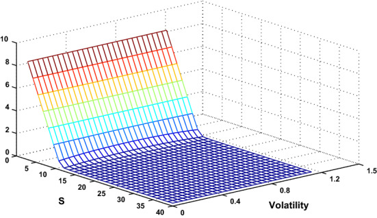
Numerical solution

In this example we study the properties of the numerical solution by studying the behavior of the first order partial derivatives $\mathrm{\Delta }=\frac{\partial \vartheta }{\partial S}$ and $\nu =\frac{\partial \vartheta }{\partial r}$. In Fig. 2, remark that when S tends to zero, $\mathrm{\Delta }$ is decreasing fast up to $-1$. On the other hand, when $S\approx K$, $\mathrm{\Delta }$ is increasing fast up to 0. As expected, the put option price tends to zero for large asset price.

Fig. 2.

The curves of $\mathrm{\Delta }=\frac{\partial \vartheta }{\partial S}$ (left) and $\nu =\frac{\partial \vartheta }{\partial r}$ (right) of the Option

Example 2

In this example we will examine the stability and the positivity of the solution to the Eq. (6.37). From Theorems 5.1 and 5.3 the solution is positive and stable if the conditions (5.22) is satisfied. The parameters considered in this example are given by:

$$\begin{array}{cc}& \gamma =0.2,T=0.25,[S_l,S_r]=[0.25,40],[r_l,r_r]=[0.002,1.2],\hfill \\ \hfill & N_t=100,K=10,\sigma =0.1,\rho =0.1,{\mu }_1={\mu }_2=1,\eta =3.\hfill \end{array}$$

In this case and using the above parameters, the condition (5.22) is as follows:

$$\begin{array}{c}\hfill \frac{\mathrm{\Delta }S}{\mathrm{\Delta }r}\le 0.0833.\end{array}$$

That means, if we take $\frac{\mathrm{\Delta }S}{\mathrm{\Delta }r}\notin \mathcal{I}=[0,0.0833]$ the solution will not be neither stable nor positive. Thus, Fig. 3 confirm this result (Figs. 4, 5 and 6).

Fig. 3.

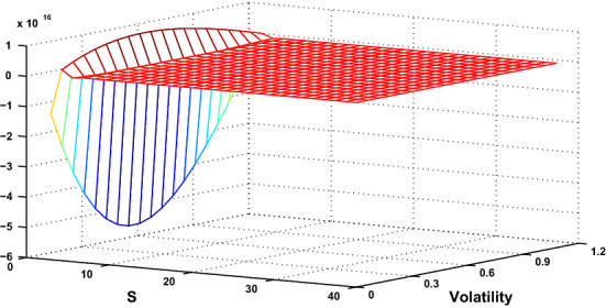
Unstable and non-positive solution for $\frac{\mathrm{\Delta }S}{\mathrm{\Delta }r}=22.1202\notin \mathcal{I}$, ($N_S=30$, $N_r=20$)

Fig. 4.

Numerical solution a$\gamma =0.2$, b$\gamma =0.5$

Fig. 5.

Numerical solution a$\gamma =0.7$, b$\gamma =0.9$

Fig. 6.

Numerical solution a$\gamma =0.99$, b$\gamma =0.9999$

Example 3

The parameters considered in this example are given by:

$$\begin{array}{cc}& T=0.25,[S_l,S_r]=[0.25,40],[r_l,r_r]=[0.002,1.2],N_S=N_r=25,N_t=100\hfill \\ \hfill & K=10,\sigma =0.9,\rho =0.9,{\mu }_1={\mu }_2=1,\eta =70.\hfill \end{array}$$

In this example, we study the numerical solution with respect the variation of $\gamma$. We plot the solution for $\gamma =0.2,0.5,0.7,0.9,0.99$.

Conclusion

The time fractional Vasicek Model is a generalized of the classical Vasicek Model. The nature of the fractional order derivative in the model makes the numerical solution more difficult to obtain than the integer order model.

In this work, we used a time splitting method to solve numerically the model. This method allowed us to obtain very satisfactory numerical results. A case with high correlation $\rho =0.9$ is considered to show the advantages of our method in controlling the perturbations coming from the mixed derivative as its well known in the literature.

Author Contributions

Each author equally contributed to this paper, and read and approved the final manuscript. All authors have read and agreed to the published version of the manuscript.

Funding

This work was funded by the Deanship of Scientific Research at Jouf University under Grant No (DSR-2021-03-03139).

Declarations

Conflict of interest

This work does not have any conflicts of interest.

References

- Ahmad B, Alsaedi A, Ntouyas SK, Tariboon J. Hadamard-type fractional differential equations inclusions and inequalities. 1. Springer; 2017. p. 414. [Google Scholar]
- Amit G, Singh J, Kumar D, Sushila An efficient analytical approach for fractional equal width equations describing hydro-magnetic waves in cold plasma. Physica A. 2019;524:563–575. doi: 10.1016/j.physa.2019.04.058. [DOI] [Google Scholar]
- Arfaoui H. Stabilization method for the Saint-Venant equations by boundary control. Transactions of the Institute of Measurement and Control. 2020;42(Issue16):3290–3302. doi: 10.1177/0142331220950033. [DOI] [Google Scholar]
- Atangana A, Baleanu D. New fractional derivatives with nonlocal and non-singular kernel: Theory and application to heat transfer model. Journal of Thermal Science. 2016;20:763–769. doi: 10.2298/TSCI160111018A. [DOI] [Google Scholar]
- Bayrak MA, Demir A, Ozbilge E. A novel approach for the solution of fractional diffusion problems with conformable derivative. Numerical Methods for Partial Differential Equations. 2021 doi: 10.1002/num.22750. [DOI] [Google Scholar]
- Benchohra M, Graef JR, Mostefai FZ. Weak solutions for boundary-value problems with nonlinear fractional differential inclusions. Nonlinear Dynamics and Systems Theory. 2011;3:227–237. [Google Scholar]
- Bensoussan A. On the theory of option pricing. Acta Applicandae Mathematicae. 1984;2:139–158. doi: 10.1007/BF00046576. [DOI] [Google Scholar]
- Black F, Scholes MS. The pricing of options and corporate liabilities. Journal of Political Economy. 1973;81:279–296. doi: 10.1086/260062. [DOI] [Google Scholar]
- Cao J, Chen Y, Wang Y, Cheng G, Barriere T, Wang L. Numerical analysis of fractional viscoelastic column based on shifted Chebyshev wavelet function. Applied Mathematical Modelling. 2021;91:374–389. doi: 10.1016/j.apm.2020.09.055. [DOI] [Google Scholar]
- Cardoso LC, Camargo RF, Dos Santos FLP, Dos Santos PC. Global stability analysis of a fractional differential system in hepatitis B. Chaos, Solitons and Fractals. 2021;143:110619. doi: 10.1016/j.chaos.2020.110619. [DOI] [Google Scholar]
- Company, R., Egorova, V. N., Jódar, L., Valls, F. F. (2020) An ETD method for American options under the Heston model. Computer Modeling in Engineering Sciences. 10.32604/cmes.2020.010208 10.32604/cmes.2020.010208. [DOI]
- Daftardar-Gejji V, Babakhani A. Analysis of a system of fractional differential equations. Journal of Mathematical Analysis and Applications. 2004;293:511–522. doi: 10.1016/j.jmaa.2004.01.013. [DOI] [Google Scholar]
- Daftardar-Gejji V, Bhalekar S. Solving multiterm linear and nonlinear diffusion wave equations of fractional order by Adomian decomposition method. Applied Mathematics and Computation. 2008;202:113–120. doi: 10.1016/j.amc.2008.01.027. [DOI] [Google Scholar]
- Dumitru B, Pshtiwan Othman M, Miguel VC, Yenny RO. Some modifications in conformable fractional integral inequalities. Advances in Difference Equations. 2020;374:1–25. [Google Scholar]
- Erdelyi, A., Magnus, W., Oberhettinger, F., Tricomi, F. G. and Research Associates (1953). In E. Robert (Ed.), Higher transcendental functions (Vol. III). Krieger Publishing Co. Inc. https://resolver.caltech.edu/CaltechAUTHORS:20140123-104529738
- Garrappa R. Exponential integrators for time-fractional partial differential equations. The European Physical Journal Special Topics. 2013;222:1915–1927. doi: 10.1140/epjst/e2013-01973-1. [DOI] [Google Scholar]
- Golub Gene H, Van Loan, Charles F. Matrix Computations. The Johns Hopkins University Press; 1996. [Google Scholar]
- Heston SL. Closed form solution for options with stochastic volatility with application to bonds and currency options. The Review of Financial Studies. 1993;6:327–343. doi: 10.1093/rfs/6.2.327. [DOI] [Google Scholar]
- Higazy M, Allehiany FM, Mahmoud EE. Numerical study of fractional order COVID-19 pandemic transmission model in context of ABO blood group. Results in Physics. 2021;22:103852. doi: 10.1016/j.rinp.2021.103852. [DOI] [PMC free article] [PubMed] [Google Scholar]
- Kilbas AA, Srivastava HM, Trujillo JJ. Theory and applications of fractional differential equations. Elsevier; 2006. [Google Scholar]
- Kaczorek T. Positive 1D and 2D systems. Springer; 2002. [Google Scholar]
- Kharrat M. Computation of conditional expectation using Malliavin Calculus under Vasicek model. Wulfenia Journal. 2014;21(4):143–152. [Google Scholar]
- Kharrat M. Closed-form solution of European option under fractional Heston model. Nonlinear Dynamics and Systems Theory. 2018;18(2):191–195. [Google Scholar]
- Kharrat M. Pricing American put option under fractional Heston model. Pramana Journal of Physics. 2021 doi: 10.1007/s12043-020-02039-z. [DOI] [Google Scholar]
- Mirrezapour SZ, Zare A, Hallaji M. A new fractional sliding mode controller based on nonlinear fractional-order proportional integral derivative controller structure to synchronize fractional-order chaotic systems with uncertainty and disturbances. Journal of Vibration and Control. 2021 doi: 10.1177/1077546320982453. [DOI] [Google Scholar]
- Moustafa M, Mohd MH, Ismail AI, Abdullah FA. Global stability of a fractional order eco-epidemiological system with infected prey. International Journal of Mathematical Modelling and Numerical Optimisation. 2021 doi: 10.1504/IJMMNO.2021.111722. [DOI] [Google Scholar]
- Owolabi KM. Numerical approach to chaotic pattern formation in diffusive predator-prey system with Caputo fractional operator. Numerical Methods for Partial Differential Equations. 2021;37:131–151. doi: 10.1002/num.22522. [DOI] [Google Scholar]
- Podlubny I. Fractional differential equations calculus. Academic Press; 1999. [Google Scholar]
- Srivastava HM, Dubey VP, Kumar R, Singh J, Kumar D, Baleanu D. An efficient computational approach for a fractional-order biological population model with carrying capacity. Chaos, Solitons & Fractals. 2020;138:109880. doi: 10.1016/j.chaos.2020.109880. [DOI] [Google Scholar]
- Vasicek O. An equilibrium characterization of the term structure. Journal of Financial Economics. 1977;5(2):177–188. doi: 10.1016/0304-405X(77)90016-2. [DOI] [Google Scholar]
- Xiaozhong Y, LifeiEmail W, Shuzhen S, Xue Z. A universal difference method for time-space fractional Black-Scholes equation. Advances in Difference Equations. 2016;2016:1–4. doi: 10.1186/s13662-016-0792-8. [DOI] [Google Scholar]
- Yu JM, Luo YW, Zhou SB, Lin XR. Existence and uniqueness for nonlinear multi-variables fractional differential equations. Nonlinear Dynamics and Systems Theory. 2011;2:213–221. [Google Scholar]
- Zhang H, Liu F, Turner I, Yang Q. Numerical solution of the time fractional Black-Scholes model governing European options. Computers and Mathematics with Applications. 2016;71(Issue 16):1772–1783. doi: 10.1016/j.camwa.2016.02.007. [DOI] [Google Scholar]