Application of hyperspectral imaging and chemometrics for variety classification of maize seeds

Abstract

Seed variety classification is important for assessing variety purity and increasing crop yield. A hyperspectral imaging system covering the spectral range of 874–1734 nm was applied for variety classification of maize seeds. A total of 12 900 maize seeds including 3 different varieties were evaluated. Spectral data of 975.01–1645.82 nm were extracted and preprocessed. Discriminant models were developed using a radial basis function neural network (RBFNN). The influence of calibration sample size on classification accuracy was studied. Results showed that with the expansion of calibration sample size, calibration accuracy varied slightly, but prediction accuracy changed from the increasing form to the stable form. Accordingly, the optimal size of the calibration set was determined. Optimal wavelength selection was conducted by loading of principal components (PCs). The RBFNN model developed on optimal wavelengths with the optimal size of the calibration set obtained satisfactory results, with calibration accuracy of 93.85% and prediction accuracy of 91.00%. Visualization of classification map of seed varieties was achieved by applying this RBFNN model on the average spectra of each sample. Besides, the procedure to determine the optimal sample quantity proposed in this study was verified by support vector machine (SVM). The overall results indicated that hyperspectral imaging was a potential technique for variety classification of maize seeds, and would help to develop a real-time detection system for maize seeds as well as other crop seeds.

Hyperspectral imaging provides an effective way for seed variety classification for assessing variety purity and increasing crop yield.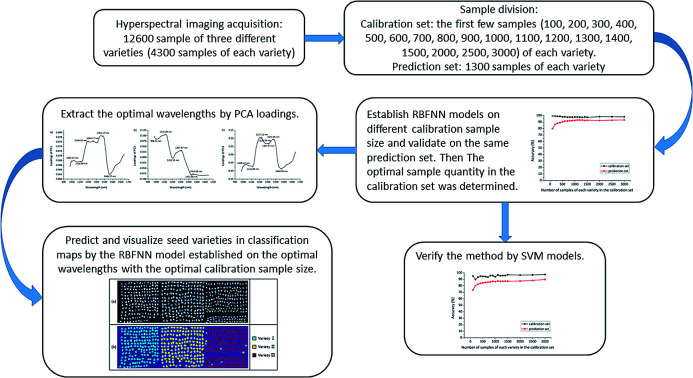

1. Introduction

Maize (Zea Mays L.), a widely cultivated crop in some parts of the world, is used for human consumption and animal feed, and can be processed into many industrial products.¹ As an essential factor for assessing the quality of maize seeds, variety purity has a profound impact on the growth and final yield of maize.² However, in the whole growth and development process, many procedures such as cultivation, harvesting, transportation, and storage, will probably result in a mixture of different varieties of maize seeds.³ And recently, this phenomenon has become increasingly aggravated because of the extensive application of seed hybrid technology. The degradation of variety purity can lead to yield loss,⁴ and will reduce farmers' economic benefits, eventually. Therefore, it is vital to strengthen purity assessment of maize seeds for quality assurance, which illustrates the great importance of variety classification of maize seeds before planting.

Several approaches have been developed and applied for variety classification of seeds, such as morphology identification, DNA molecular marker technology, and protein electrophoresis.^5–7 But most of these traditional methods have some limitations such as being time-consuming, and requiring specialized instruments and skilled operators, which restricts their application in on-line and large-scale detection in modern seed industry. To overcome these shortcomings, great focus has been put on developing fast, non-destructive and reliable methods for seed identification and classification. In this study, rapid variety discrimination based on hyperspectral imaging and chemometrics was investigated.

Hyperspectral imaging, an emerging technique that integrates both spectroscopic and imaging techniques in one system,⁸ has the advantage of providing external (surface and spatial) and internal quality information simultaneously. Each pixel within the image contains a spectrum at the spectral range of the hyperspectral imaging system. By combining the corresponding spatial distribution of each pixel, visualization of sample features (physical, chemical, and category) can be realized.⁹ Previous studies explored the possibility of applying hyperspectral imaging for variety classification of maize seeds. Zhang et al.¹⁰ employed hyperspectral imaging to differentiate 330 maize seeds, including 6 varieties, and the optimal recognition accuracy of 98.89% was achieved by the least squares-support vector machine (LS-SVM) model based on data fusion. Wang et al.¹¹ combined spectral data with textural features obtained from hyperspectral images for classifying 400 maize seeds, including 3 varieties, achieving an accuracy of 88.89%. Huang et al.⁴ employed hyperspectral imaging for classifying 2000 maize seeds, including 4 varieties that were harvested in different years, and the prediction accuracy of the LS-SVM model coupled with model updating reached 94.4%. Moreover, Huang et al.¹² applied hyperspectral imaging to classify 1632 maize seeds, including 17 varieties, and the test accuracy of the LS-SVM model based on the combination of spectral and image features coupled with feature transformation was over 90%.

The successful application of hyperspectral imaging greatly depends on the established calibration models with high accuracy and robustness, which is particularly important for real-time and on-line detection. In general, the above researches mainly focused on effective variable extraction, data fusion, and model updating to optimize the discriminant models for maize seeds. However, besides the mentioned approaches, the number of samples in the calibration set was also reported to be an essential factor affecting the accuracy and robustness of the established calibration models.¹³ Kuang¹⁴ evaluated the effect of the number of fresh soil samples in the calibration set on the prediction error considered as root mean square error of prediction (RMSEP) for farm-scale modelling of total nitrogen, organic carbon and moisture content. Results illustrated that the calibration models built by the large-size calibration set would result in lower RMSEP than those built by the small-size calibration set for all the three soil properties investigated. To our knowledge, however, there is no specific research on how the number of maize seeds in the calibration set affects the classification ability of the discriminant models. In general, a relatively large-size calibration set may be a superior option to describe sample features and may exhibit better prediction capability than a small-size one, for the wider range of variation in the calibration samples. However, the complexity of the discriminant models and the cost of analysing will be considerably higher. The balance between the expected classification accuracy and modelling complexity is worth consideration. Thus, the main purpose of this study was to evaluate the influence of calibration sample size on classification accuracy. To better carry out this work, a large number of maize seed samples should be included. Therefore, a total of 12 900 maize seed samples of 3 different varieties were collected in this research.

In all, this study was performed to achieve these objectives: (1) to assess the potential of applying hyperspectral imaging and chemometric methods for differentiating maize seeds, (2) to evaluate the influence of calibration sample size on classification accuracy, (3) to identify optimal wavelengths related to category information, (4) to develop radial basis function neural network (RBFNN) models on optimal wavelengths with the optimal size of the calibration set, and (5) to visualize the classification map of maize seeds for better purity assessment and quality monitoring.

2. Materials and methods

2.1. Sample preparation

A total of 12 900 maize seeds including 3 different varieties (4300 maize seeds of each variety) were kindly provided by a commercial seed company (Jiudingjiusheng Seed Industrial Co., Ltd, Beijing, China). Seed varieties were coded as no. 106101, no. 106100 and no. 7879 instead of their original chemical names to protect the company law. They were collected and naturally dried in 2016, and stored in kraft paper bags. And the three varieties were recorded as variety I, variety II and variety III in this study, respectively. No apparent injury was seen for all the collected samples.

2.2. Hyperspectral imaging system

Hyperspectral images of maize seeds were collected by a line-scan hyperspectral imaging system in the NIR range (874–1734 nm with 256 bands). This hyperspectral imaging system is composed of an imaging spectrograph (ImSpector N17E; Spectral Imaging Ltd., Oulu, Finland), a 320 × 256 InGaAs camera (Xeva 992; Xenics Infrared Solutions, Leuven, Belgium) with a camera lens (OLES22; Specim, Spectral Imaging Ltd.), an illumination unit of two 150 W tungsten halogen lamps (Fiber-Lite DC950 Illuminator; Dolan Jenner Industries Inc., Boxborough, MA, USA), a conveyer belt driven by a stepper motor (Isuzu Optics Corp., Taiwan, China), and a computer equipped with a matched data acquisition software (Xenics N17E; Isuzu Optics Corp., Taiwan, China). The whole system was placed in a dark room.

2.3. Image acquisition and correction

Image acquisition was carried out at room temperature. At each time, maize seeds were placed on a black plate without overlapping each other. The plate was then put on the conveyer belt for scanning. In order to obtain clear images without deformation, the height between the camera lens and the samples was set at 29 cm and the exposure time of the camera was set at 3 ms. The system scanned the samples line by line along the Y-axis. And the samples were moved along the X-axis at a constant speed of 33.8 mm s⁻¹.

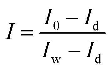
The raw hyperspectral images of the samples were corrected using two reference standards: the white reference image and the dark reference image, obtained under the same condition as sample image acquisition. The white reference image was obtained using a white Teflon bar of nearly 100% reflectance, and the dark reference image was acquired by turning off the light source and completely covering the lens with its opaque cap. Then the corrected image was calculated by the following equation:

1

where I is the corrected image, I₀ is the raw image, I_d is the dark reference image, and I_w is the white reference image.

2.4. Spectral data extraction

To extract spectral data, image segmentation was carried out first, the main purpose of which was to separate only the maize seed samples from the background. Region of interest (ROI) was defined as the entire sample region of each maize seed. So totally, 12 900 ROIs were used in extracting spectral data from the corrected hyperspectral images. The average spectra at 874–1734 nm of all pixels within each ROI were then calculated to represent the corresponding seed sample.

3. Data analysis

3.1. Principal component analysis

Principal component analysis (PCA) is a widely used multivariate statistical method for qualitative analysis of spectral data.¹⁵ The principle of PCA is to replace the original variables with a group of new variables called principal components (PCs). Each PC is a linear transformation of the original variables and PCs are arranged in descending order of explained variance. The first few PCs explaining the most variance of the original data were often used to form scores scatter plot for identifying patterns in data, especially for classification issues.^8–10 In addition, contribution of individual wavelength could be reflected by corresponding loadings of the PCs.¹⁶ Hence, loadings of the first few PCs with the greatest contribution could be used to identify important wavelengths.¹⁷ In this study, scores scatter plot was drawn to show the grouping, similarities and differences among maize seed samples of different varieties. And optimal wavelength selection was conducted according to PCA loadings.

3.2. Calibration methods

3.2.1. Radial basis function neural network

Radial basis function neural network (RBFNN) is a feed-forward network that has an input layer, a single hidden layer and an output layer. RBFNN uses radial basis function (RBF) as the activation function of the neurons in the hidden layer, and the output layer is a linear combiner.¹⁵ RBFNN is especially suitable for solving classification issues with fast convergence speed and the ability to approximate any continuous functions at arbitrary precision.^18,19 In this research, RBFNN models were established for variety discrimination of maize seeds. Model performance were evaluated in terms of classification accuracy, including calibration accuracy and prediction accuracy.

3.2.2. Support vector machine

Support vector machine (SVM) is a machine learning algorithm based on structural risk minimisation. SVM works by mapping data of low dimension space into a higher dimension space in which a separating hyperplane is constructed to realize linear classification. By introducing kernel function, the computational complexity will be effectively reduced.²⁰ In this research, SVM was used to verify whether the method to determine the optimal size of calibration set proposed from RBFNN models could be applied to other discriminant models.

3.3. Software

Extraction of spectral data and spatial information was carried out on ENVI 5.1 (ITT Visual Information Solutions, Boulder, CO, USA). Implementation of PCA and establishment of RBFNN and SVM models were conducted on MATLAB R2017b (The MathWorks, Natick, MA, USA).

3.4. Visualization of classification map

Each pixel in hyperspectral images contains a spectrum covering the whole spectral range of the hyperspectral imaging system. The advantage of acquiring spectral and spatial information simultaneously provides the feasibility of predicting chemical, physical and category information of each pixel within the samples, based on the established calibration models.²¹ However, as for variety classification of maize seeds, it was not necessary to present the category information of each pixel, so the average spectra of all pixels within the sample were used for visualization in this study. Results of visualization highly depended on the average spectra of each sample and performance of the calibration models. Random noise existing in the average spectra would cause unstable or inaccurate predicting results, so it should be reduced before visualizing. Besides, the established calibration models were supposed to be robust and reliable. Thus, the general steps of image visualization were as follows:

(1) Samples were isolated from the background and the sample region of each maize seed was defined as an ROI.

(2) Spectral data were extracted from the predefined ROI, and the average spectra of each ROI were calculated and preprocessed.

(3) Calibration models were developed on optimal wavelengths with the optimal number of samples in the calibration set.

(4) The category value of each ROI was predicted by using the corresponding average spectra and the established calibration models.

(5) By describing different varieties of maize seeds with specific colours, classification maps were formed.

Visualization of classification map made it possible to visualize category information of the samples, which was beneficial for convenient and intuitive discrimination of seed variety in crop seed industry, especially for a large quantity of samples to be classified.

4. Results and discussion

4.1. Spectral profile

Since the head and the end of the spectrum contained obvious noise, only spectra in the range of 975.01–1645.82 nm preprocessed by wavelet transform (WT) using Daubechies 8 with a decomposition level of 3 were used for further analysis to obtain reliable and accurate results.

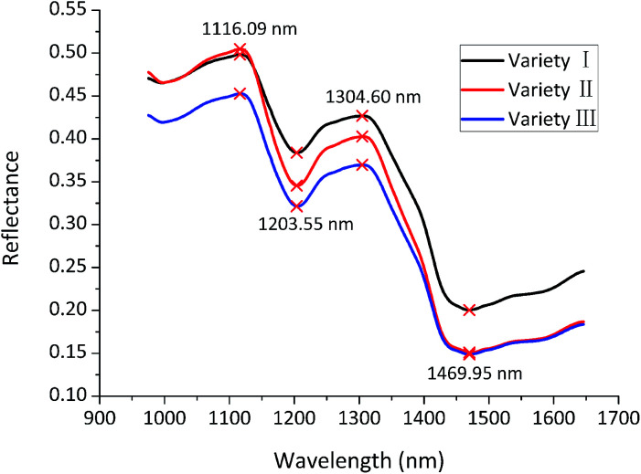
The average reflectance spectra of three varieties were calculated and presented in Fig. 1. The average spectra of three varieties exhibited quite similar trends, but differences in reflectance values could also be seen, due to different composition and physicochemical characteristics of three maize seed varieties. The peak at 1116.09 nm may correspond to the C–H groups from lipids.²² The valley at 1203.55 nm may be associated with 2nd overtone of C–H.²³ The peak at 1304.60 nm may be assigned to combination between the 1st overtone of N–H stretching with the fundamental N–H in-plane bending and C–N stretching with N–H in-plane bending vibrations.²⁴ The valley at 1469.95 nm may arise from 1st overtone of N–H.²³ However, variety classification couldn't be achieved only by the differences of the average spectra. Therefore, latent features of the average spectra needed to be excavated for variety discrimination.

Fig. 1. Average reflectance spectra of maize seeds of three varieties in the range of 975.01–1645.82 nm.

4.2. Principal component analysis

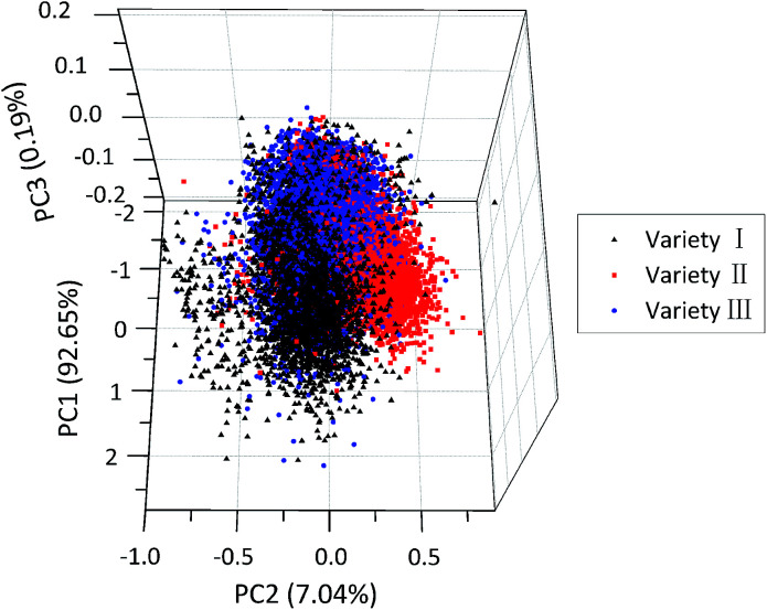
For qualitatively identifying patterns in different varieties of maize seeds, PCA was performed on the preprocessed spectra collected from all samples. Results showed that the variance explained by the first three PCs was 92.65%, 7.04% and 0.19% of the total variance, respectively. That is to say, the sum of the variance of the first three PCs accounted for 99.88% of the total variance of the spectral data, so it might be a reasonable way to recognize patterns in the tested samples. The distribution of all the samples in the new coordinate system was defined by the first three PCs. As shown in Fig. 2, maize seeds of different varieties were well grouped and had their cluster centre, respectively. However, there were overlaps among sample points of different varieties, especially between variety III and other two varieties, and some sample points were away from their corresponding cluster centre. This demonstrated that it was hard to accurately differentiate all kinds of samples in the qualitative way, especially for samples near the borders. Therefore, models for quantitative discrimination of maize seeds were needed.

Fig. 2. Scores scatter plot of the first three PCs of maize seeds of three varieties.

4.3. Influence of calibration sample size on classification accuracy

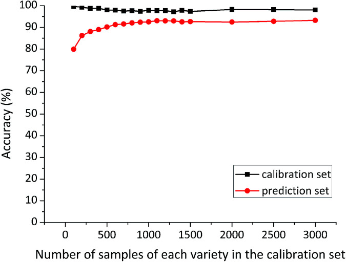
At each time, the first several samples (sample size of 100, 200, 300, 400, 500, 600, 700, 800, 900, 1000, 1100, 1200, 1300, 1400, 1500, 2000, 2500, 3000) of each variety were selected from the large sample pool into the calibration set. The number of samples in the calibration set was served as the only variable, while other factors were kept unchanged. Special attention was paid to ensuring that the prediction set was composed of the same 3900 maize seeds (1300 samples of each variety) for each model. Classification accuracy of RBFNN models developed on different size of the calibration sets is shown in Fig. 3.

Fig. 3. Classification results of RBFNN models developed on different size of the calibration sets.

Calibration accuracy of these RBFNN models varied slightly with different size of the calibration sets, but it remained over 97%. Whereas, prediction accuracy of RBFNN models presented an increasing trend from the small-size calibration set to the large-size one. In addition, prediction accuracy grew fast with the number of calibration samples of each variety rising from 100 to 600, while a slow increasing could be observed between 600 and 1100 calibration samples of each variety. Surprisingly, prediction accuracy based on calibration sets containing more than 1100 samples of each variety remained stable. This phenomenon indicated that the specific 1100 samples of each variety might contain important information for discrimination. Detailed classification results of RBFNN models based on 3000 and 1100 samples of each variety in the calibration set are shown in Table 1.

Classification results of RBFNN models based on 3000 and 1100 samples of each variety in the calibration set.

Samples of each variety in the calibration set		Calibration				Prediction
		1	2	3	Accuracy	1	2	3	Accuracy
3000	1	2931	12	57	97.70%	1180	36	84	90.77%
	2	11	2961	28	98.70%	33	1210	57	93.08%
	3	45	24	2931	97.70%	38	15	1247	95.92%
	Total				98.03%				93.26%
1100	1	1070	5	25	97.27%	1192	25	83	91.69%
	2	7	1084	9	98.55%	42	1209	49	93.00%
	3	22	6	1072	97.45%	51	21	1228	94.46%
	Total				97.76%				93.05%

For the large-size calibration model (3000 samples of each variety in the calibration set), classification accuracy was 98.03% for the calibration set and 93.26% for the prediction set. It could be explained that the abundant information related to internal quality was contained in the large number of maize seeds in the calibration set. Nevertheless, a small minority of the samples were identified as the wrong variety. In both calibration and prediction sets, samples of variety I and variety II were more likely to be misclassified as variety III, and samples of variety III were more likely to be misclassified as variety I. The small-size calibration model (1100 samples of each variety in the calibration set) obtained similar results, with accuracy of 97.76% for the calibration set and 93.05% for the prediction set, which was relatively satisfactory. It was worth noting that the misclassifying phenomenon matched with that of the large-size calibration model. The composition and physicochemical characteristics between variety III and other two varieties might be more similar.

The overall results indicated that it was feasible to use hyperspectral imaging technique combined with RBFNN models for seed variety discrimination. Additionally, classification results of RBFNN models (calibration accuracy of 98.03% and prediction accuracy of 93.26% based on 3000 samples of each variety in the calibration set, and calibration accuracy of 97.76% and prediction accuracy of 93.05% based on 1100 samples of each variety in the calibration set) demonstrated that using relatively small number of samples to establish calibration model could achieve similar prediction capability with that based on large number of samples. The reason might be that the 1100 calibration samples of each variety involved sufficient samples to explain the seed variability for discrimination. In addition, significant reduction in sample size of the calibration set helped to build a much simpler discriminant model with lower computational complexity and higher efficiency. Therefore, the optimal size of the calibration set was determined as 1100 samples of each variety.

4.4. Optimal wavelength selection

The large amount of data generated in hyperspectral images is always of high dimensions, which is considered to be a major problem in analysis and application. The contiguous wavelengths in hyperspectral images are highly correlated and may contain redundant information, which will result in high computational cost and generate relatively complex and unstable models as well. Optimal wavelength selection is a useful tool to reduce the high dimensionality of the extracted spectral data. Using the informative wavelengths could help to speed up the detection and make a simpler discriminant model. Ideally, the classification accuracy should be unchanged or degraded within an acceptable range, while the computational cost is greatly reduced.⁸ In this study, optimal wavelength selection was implemented for dimension reduction and to recognize the most relevant wavelengths for discrimination.

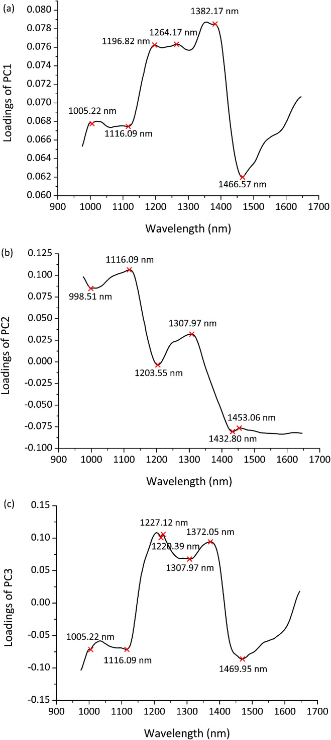
The first three PCs explained most of the total variance (PC1 = 92.65%, PC2 = 7.04%, PC3 = 0.19%). So the PCA loadings of the first three PCs were employed to identify the important wavelengths with the greatest contribution for discrimination. Fig. 4(a–c) shows the PCA loading plots of the first three PCs in the entire spectral range. Wavelengths located at peaks and valleys were chosen as the informative wavelengths of each PC. In total, 15 wavelengths (998.51, 1005.22, 1116.09, 1196.82, 1203.55, 1220.39, 1227.12, 1264.17, 1307.97, 1372.05, 1382.17, 1432.80, 1453.06, 1466.57, 1469.95 nm) were selected to represent the full spectra for further tests to identify and classify maize seeds with reduced data processing.

Fig. 4. PCA loading plots and the informative wavelengths of (a) PC1, (b) PC2, (c) PC3.

4.5. RBFNN models developed on optimal wavelengths

As a consequence of selecting optimal wavelengths by PCA loadings and average reflectance spectra, the number of wavelengths was reduced. Then these selected optimal wavelengths carrying the most important information were regarded as the input variables to build RBFNN model with the optimal number of calibration samples. Besides, to further evaluate the representativeness of the chosen optimal size of the calibration set, RBFNN model based on the optimal wavelengths with 3000 samples of each variety in the calibration set was established as a comparison. Classification results of RBFNN models developed on these optimal wavelengths with 1100 and 3000 samples of each variety in the calibration set are shown in Table 2.

Classification results of RBFNN models developed on optimal wavelengths with 3000 and 1100 samples of each variety in the calibration set.

Samples of each variety in the calibration set		Calibration				Prediction
		1	2	3	Accuracy	1	2	3	Accuracy
3000	1	2799	48	153	93.30%	1176	49	75	90.46%
	2	44	2907	49	96.90%	40	1196	64	92.00%
	3	166	65	2769	92.30%	83	37	1180	90.77%
	Total				94.17%				91.08%
1100	1	1010	20	70	91.82%	1184	49	67	91.08%
	2	19	1063	18	96.64%	46	1195	59	91.92%
	3	66	10	1024	93.09%	87	43	1170	90.00%
	Total				93.85%				91.00%

For the large-size calibration model (3000 samples of each variety in the calibration set), in comparison with RBFNN model based on the full spectra, model performance developed on optimal wavelengths was slightly worse, but classification accuracy of 94.17% for the calibration set and 91.08% for the prediction set was comparatively receivable. Surprisingly, both based on optimal wavelengths, the small-size calibration model (1100 samples of each variety in the calibration set) achieved quite approximate results with the large-size calibration model. Classification results of 93.85% for the calibration set and 91.00% for the prediction set were relatively acceptable, which further validated the representativeness of the chosen optimal size of the calibration set. And it was worth noting that the number of wavelengths reduced from 200 to 15, which only accounted for 7.50% of the total wavelengths. In this point of view, the simplified discriminant model was better than the RBFNN model developed on the full spectra. Meanwhile, the similar phenomenon was observed in Table 2 as in Table 1 that in both calibration and prediction sets, samples of variety I and variety II were more likely to be misclassified as variety III, and samples of variety III were more likely to be misclassified as variety I.

In all, simpler discriminant models were obtained with signification reduction in computational task by using the selected optimal wavelengths. Besides, the small-size RBFNN model based on these optimal wavelengths with 1100 samples of each variety in the calibration set was much simpler than all other corresponding RBFNN models, and its classification results were relatively satisfactory. The overall results indicated that it was an effective way to select optimal wavelengths to build discriminant models by PCA loadings, with great reduction in computational cost and relatively acceptable model performance.

4.6. Image visualization of seed variety

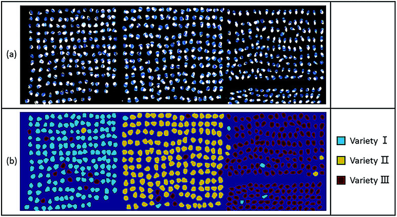
It can be very challenging to visualize the high dimensional spectral data.⁸ Since determining the optimal size of the calibration set and optimal wavelengths was proved to be useful for dimension reduction, RBFNN model developed on optimal wavelengths with 1100 samples of each variety in the calibration set was applied to predict the variety of each sample in hyperspectral images. The average spectra of ROIs extracted from the hyperspectral images were smoothed by WT using Daubechies 8 with a decomposition level of 3. In classification maps, maize seeds of variety I, variety II, and variety III were visualized in blue, yellow and red, respectively. Fig. 5(a) shows three randomly selected grayscale maps of maize seeds of three varieties, respectively, while Fig. 5(b) shows the corresponding classification maps. Maize seed samples were successfully separated from the background. However, a small number of maize seeds were misclassified, which indicated that a robust, accurate and reliable calibration model was needed. On the other hand, the visualization results were quite encouraging that most of the maize seed samples were correctly identified and could easily be differentiated as one variety from another, which illustrated the feasibility of using hyperspectral imaging for classifying and visualizing varieties of maize seeds conveniently and intuitively. Accordingly, visualization of classification map was beneficial for purity assessment and quality monitoring in modern crop seed industry, especially for a large quantity of samples to be identified. A real-time detection system could be developed for maize seeds and other crop seeds.

Fig. 5. (a) Grayscale maps and (b) classification maps of maize seeds of three varieties.

4.7. Verification by SVM models

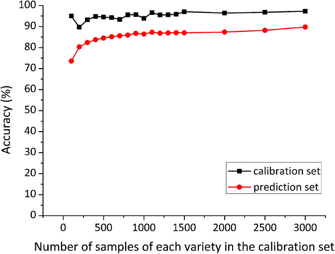
In order to explore whether the conclusion drawn from RBFNN could also be applied to other discriminant models, SVM was used to verify the repeatability of the method proposed to select the optimal number of samples in the calibration set. The composition of sample sets in SVM models was the same as that in RBFNN models. The first several samples (sample quantity of 100, 200, 300, 400, 500, 600, 700, 800, 900, 1000, 1100, 1200, 1300, 1400, 1500, 2000, 2500, 3000) of each variety constituted the calibration sets, and the prediction set was composed of the rest 3900 samples (1300 samples of each variety). Classification accuracy of SVM models developed on different size of the calibration sets is shown in Fig. 6.

Fig. 6. Classification results of SVM models developed on different size of calibration sets.

Calibration accuracy of SVM models on the full spectra remained over 90% except the model with 200 samples of each variety in the calibration set. In particular, calibration accuracy of SVM models developed on more than 1100 samples of each variety in the calibration set were higher than 95.50%. Prediction accuracy of SVM models showed a similar trend with that of RBFNN models, which improved along with the increase in the number of samples in the calibration sets, until the stable point was reached. For the discriminant model developed on 1100 samples of each variety, classification results of SVM models were a little worse than the corresponding RBFNN model, with calibration accuracy of 96.61% and prediction accuracy of 87.31%.

SVM models with 3000 and 1100 samples of each variety in the calibration set were also established on the selected optimal wavelengths, respectively. Detailed results are shown in Table 3. The simplified models were slightly worse than SVM models developed on the full spectra. But the results were acceptable since the number of input variables was greatly reduced.

Classification results of SVM models developed on optimal wavelengths with 3000 and 1100 samples of each variety in the calibration set.

Samples of each variety in the calibration set		Calibration				Prediction
		1	2	3	Accuracy	1	2	3	Accuracy
3000	1	2743	39	218	91.43%	1099	58	143	84.54%
	2	39	2906	55	96.87%	56	1162	82	89.38%
	3	181	52	2767	92.23%	117	36	1147	88.23%
	Total				93.51%				87.38%
1100	1	995	17	88	90.45%	1079	58	163	83.00%
	2	11	1072	17	97.45%	69	1156	75	88.92%
	3	83	22	995	90.45%	160	50	1090	83.85%
	Total				92.79%				85.26%

5. Discussion

Considering the techniques and methods used in this study, the great potential of applying hyperspectral imaging for variety classification of maize seeds was mainly based on the following points:

Firstly, measurement by near-infrared spectroscopy only focuses on a relatively small part of the sample being analysed to obtain the average values of quality information.²⁵ And uneven distribution of chemical constituents within the sample would cause much error. However, hyperspectral imaging obtained the spectrum of each pixel within the entire sample. Furthermore, by combining the spatial information acquired by the hyperspectral imaging system, the position of each sample could be fixed and the corresponding variety could be presented in classification maps, showing a great advantage over near-infrared spectroscopy. In a previous research, the variety of every single pixel within the sample was predicted and visualized.¹¹ However, considering that there was no need to know the exact category information of each pixel, the average spectra of the samples were more suitable for prediction and visualization. In addition, the ability of identifying and visualizing a large number of samples simultaneously further confirmed the efficacy of using hyperspectral imaging for real-time detection.

Secondly, visualization effects closely related to the performance of the developed calibration models, which were associated with the spectral features of a certain number of calibration samples. The influence of calibration sample size on classification accuracy was investigated. The trends of classification accuracy were used to identify the optimal size of the calibration set. By developing calibration models on the optimal number of calibration samples, prediction results were comparatively satisfactory and heavy computational task was avoided in the meanwhile. Besides, to explore whether the method to determine the optimal sample quantity could be applied to other calibration methods, SVM was used for verification. Note that although 1100 samples of each variety were considered to be appropriate for building calibration models in this study, it is recommended to identify the number of calibration samples in terms of required accuracy in practical tests.

Thirdly, a major problem was that the spectral data extracted from hyperspectral images were quite large, and were suffered from collinearity and redundancy. Dealing with such data generated heavy cost of computation and had high requirements of analysing hardware. Optimal wavelength selection was a useful tool to reduce the amount and redundancy of data, and helped to build a robust and simple model. Moreover, the computational cost was also reduced, corresponding to lower requirements of analysing.

Visualization of seed variety was based on the robust and representative calibration model developed on the optimal size of calibration samples and optimal wavelengths. Satisfactory performance of visualization verified the feasibility of using hyperspectral imaging to differentiate and visualize varieties of maize seeds, providing an efficient way for seed purity assessment and quality monitoring in maize seed industry. In addition, by combining assessment of chemical composition, viability, germination ability, insect damage and diseases, it was possible to develop a real-time system for comprehensive quality monitoring for maize seeds in the future, as well as for other crop seeds.

6. Conclusions

In this study, a hyperspectral imaging system covering the spectral range of 874–1734 nm was applied to achieve rapid and non-destructive variety classification of maize seeds. A total of 12 900 maize seeds of 3 different varieties were investigated. By evaluating the influence of calibration sample size on classification accuracy, the optimal size of the calibration set was determined as 1100 samples of each variety. The optimal wavelengths selected by the loadings of the first three PCs were used to build RBFNN models. Based on the optimal wavelengths, the small-size calibration model (1100 samples of each variety in the calibration set) obtained similar results with the large-size calibration model (3000 samples of each variety in the calibration set), with calibration accuracy of 93.85% and prediction accuracy of 91.00%. The classification results were comparatively satisfactory, in terms of reducing modelling complexity and maintaining acceptable classification accuracy. Besides, the procedure to determine the optimal sample quantity was verified by SVM method. But for the discriminant models developed on the optimal sample quantity with 1100 samples of each variety in the calibration set, RBFNN model performed better than the corresponding SVM model. Thus, the variety of each maize seed in the hyperspectral images was predicted by the simplified RBFNN model and was intuitively visualized in the classification maps, providing a quite simple way for real-time detection of seed varieties, especially for a large quantity of samples to be classified. The overall results indicated that using hyperspectral imaging and chemometrics for variety classification was promising, but further improvement needs to be explored to obtain better classification performance, and additional attention should be paid on applying this technique in on-line detection at industrial scale. Furthermore, quantitative analysis in biochemical compositions of maize seeds and further reduction and validation of informative wavelengths may be beneficial for further research on variety identification mechanism.

Conflicts of interest

There are no conflicts to declare.

References

- Ambrose A. Kandpal L. M. Kim M. S. Lee W. H. Cho B. K. Infrared Phys. Technol. 2016;75:173–179. [Google Scholar]
- Rahman A. Cho B. K. Seed Sci. Res. 2016;26:285–305. doi: 10.1017/S0960258516000234. [DOI] [Google Scholar]
- Yang X. Hong H. You Z. Cheng F. Sensors. 2015;15:15578–15594. doi: 10.3390/s150715578. [DOI] [PMC free article] [PubMed] [Google Scholar]
- Huang M. Tang J. Yang B. Zhu Q. Comput. Electron. Agric. 2016;122:139–145. doi: 10.1016/j.compag.2016.01.029. [DOI] [Google Scholar]
- Zhao T. Wang Z. T. Branford-white C. J. Xu H. Wang C. H. Plant Biol. 2011;13:940–947. doi: 10.1111/j.1438-8677.2011.00455.x. [DOI] [PubMed] [Google Scholar]
- Ye S. Wang Y. Huang D. Li J. Gong Y. Xu L. Liu L. Sci. Hortic. 2013;155:92–96. doi: 10.1016/j.scienta.2013.03.016. [DOI] [Google Scholar]
- Shuaib M. Zeb A. Ali Z. Ali W. Ahmad T. Khan I. Afr. J. Biotechnol. 2007;6:497–500. [Google Scholar]
- Kamruzzaman M. Barbin D. Elmasry G. Sun D. W. Allen P. Innovative Food Sci. Emerging Technol. 2012;16:316–325. doi: 10.1016/j.ifset.2012.07.007. [DOI] [Google Scholar]
- Zhang C. Guo C. Liu F. Kong W. He Y. Lou B. J. Food Eng. 2016;179:11–18. doi: 10.1016/j.jfoodeng.2016.01.002. [DOI] [Google Scholar]
- Zhang X. Liu F. He Y. Li X. Sensors. 2012;12:17234–17246. doi: 10.3390/s121217234. [DOI] [PMC free article] [PubMed] [Google Scholar]
- Wang L. Sun D. W. Pu H. Zhu Z. Food Analytical Methods. 2016;9:225–234. doi: 10.1007/s12161-015-0160-4. [DOI] [Google Scholar]
- Huang M. He C. Zhu Q. Qin J. Appl. Sci. 2016;6:183. doi: 10.3390/app6060183. [DOI] [Google Scholar]
- Kuang B. Mouazen A. M. Eur. J. Soil Sci. 2011;62:629–636. doi: 10.1111/j.1365-2389.2011.01358.x. [DOI] [Google Scholar]
- Kuang B. Mouazen A. M. Eur. J. Soil Sci. 2012;63:421–429. doi: 10.1111/j.1365-2389.2012.01456.x. [DOI] [Google Scholar]
- Zhang C. Wang C. Liu F. He Y. J. Spectrosc. 2016;2016:1–7. [Google Scholar]
- Serranti S. Gargiulo A. Bonifazi G. J. Near Infrared Spectrosc. 2012;20:573–581. doi: 10.1255/jnirs.1016. [DOI] [Google Scholar]
- Kamruzzaman M. Elmasry G. Sun D. W. Allen P. J. Food Eng. 2011;104:332–340. doi: 10.1016/j.jfoodeng.2010.12.024. [DOI] [Google Scholar]
- del Moral F. G. Guillén A. del Moral L. G. O'Valle F. Martínez L. del Moral R. G. J. Food Eng. 2009;90:540–547. doi: 10.1016/j.jfoodeng.2008.07.027. [DOI] [Google Scholar]
- Li X. Wu M. Lu G. Yan Y. Liu S. IET Renew. Power Gener. 2015;9:323–330. doi: 10.1049/iet-rpg.2013.0392. [DOI] [Google Scholar]
- Dong J. J. Li Q. L. Yin H. Zhong C. Hao J. G. Yang P. F. Tian Y. H. Jia S. R. Food Chem. 2014;161:376–382. doi: 10.1016/j.foodchem.2014.04.006. [DOI] [PubMed] [Google Scholar]
- Zhang C. Jiang H. Liu F. He Y. Food Bioprocess Technol. 2017;10:213–221. doi: 10.1007/s11947-016-1809-8. [DOI] [Google Scholar]
- Marques A. S. Castro J. N. F. Costa F. J. Neto R. M. Lima K. M. G. Microchem. J. 2016;124:306–310. doi: 10.1016/j.microc.2015.09.006. [DOI] [Google Scholar]
- Ribeiro J. S. Ferreira M. M. Salva T. J. Talanta. 2011;83:1352–1358. doi: 10.1016/j.talanta.2010.11.001. [DOI] [PubMed] [Google Scholar]
- Daszykowski M. Wrobel M. S. Czarnik-Matusewicz H. Walczak B. Analyst. 2008;133:1523–1531. doi: 10.1039/B803687J. [DOI] [PubMed] [Google Scholar]
- Zhang C. Wang Q. Liu F. He Y. Xiao Y. Measurement. 2017;97:149–155. doi: 10.1016/j.measurement.2016.10.058. [DOI] [Google Scholar]