Reflection on modern methods: combining weights for confounding and missing data

Abstract

Inverse probability weights are increasingly used in epidemiological analysis, and estimation and application of weights to address a single bias are well discussed in the literature. Weights to address multiple biases simultaneously (i.e. a combination of weights) have almost exclusively been discussed related to marginal structural models in longitudinal settings where treatment weights (estimated first) are combined with censoring weights (estimated second). In this work, we examine two examples of combined weights for confounding and missingness in a time-fixed setting in which outcome or confounder data are missing, and the estimand is the marginal expectation of the outcome under a time-fixed treatment. We discuss the identification conditions, construction of combined weights and how assumptions of the missing data mechanisms affect this construction. We use a simulation to illustrate the estimation and application of the weights in the two examples. Notably, when only outcome data are missing, construction of combined weights is straightforward; however, when confounder data are missing, we show that in general we must follow a specific estimation procedure which entails first estimating missingness weights and then estimating treatment probabilities from data with missingness weights applied. However, if treatment and missingness are conditionally independent, then treatment probabilities can be estimated among the complete cases.

Key Messages.

• Inverse probability weighting can be used to address multiple sources of bias simultaneously if the weights are constructed and combined appropriately.

• To address confounding and missing data bias, weights are constructed as the product of two components: (i) a missingness probability; and (ii) a treatment probability.

• Neither component typically includes the outcome, so estimation of the combined weights when only outcome data are missing is straightforward.

• When confounder data are missing, treatment probabilities must generally be estimated using data weighted to correct for missingness, unless it is assumed that missingness and treatment are conditionally independent.

Introduction

Inverse probability weighted (IPW) estimators are commonly used in epidemiological analysis.¹ Historically developed for population sampling,² IPW has since been extended to address confounding,^3–5 censoring (i.e. selection),^6,7 missing data^8–10 and generalizability.^11–13 Estimation and application of weights to address a single bias are well discussed in the literature^6,10,12,14; however, guidance on the construction of weights to account for multiple biases simultaneously, such as the order in which weights should be estimated, is more limited. Most examples of combining weights come from time-varying settings, ^e.g.1,15 where treatment weights to address confounding are combined with weights to address potentially informative censoring (a type of missingness weight). In these examples, the treatment weights are estimated before estimating the missingness weights. In this work, we show that the order of estimation of weights (i.e. whether missingness weights should be estimated before or after treatment weights) requires careful consideration of the underlying causal structure and, in some settings, the missingness weights must be used in the estimation of the treatment weights to avoid bias. We examine two examples in which we construct weights that account for both confounding and missing data in a time-fixed setting and the required order for estimating the weights differs.

Notation and estimand

In a cohort study of subjects randomly selected from a target population, let index $i$ denote subjects, $X_i$ denote a time-fixed categorical treatment assessed at baseline and $Y_i$ denote a binary or continuous outcome observed by the end of follow-up. We assume subjects are independent and identically distributed and, for notational simplicity, we drop the subject-level index. The estimand (i.e. parameter of interest) is the marginal expectation of the outcome under different treatments, $E\left[Y^x\right]$, where $Y^x$ is the potential outcome that would occur if the treatment were set to $x$.^14,16 For many epidemiological studies, the estimand is a contrast of the mean potential outcomes under two treatments (e.g. $E\left[Y^1\right]-E\left[Y^0\right]$). We focus here on estimation of the marginal mean outcome under a fixed treatment (e.g. $E\left[Y^1\right]$), as any contrast of marginal mean outcomes between treatments will be valid when $E\left[Y^x\right]$ is valid for each value of $X$.

Identification

First, we discuss identification of the estimand when confounding is present and all data are fully observed (i.e. no missing data). To estimate causal effects, it is necessary to assume that a set of untestable identification conditions holds.¹⁷ One sufficient set of conditions comprises conditional exchangeability with positivity and causal consistency. Conditional exchangeability^3,14 means that, conditional on a set of measured common causes of treatment and outcome ($\mathit{Z}$), the potential outcomes are independent of treatment (i.e. $Y^x\coprod X|\mathit{Z}$) such that $E\left[Y^x|\mathit{Z}\right]=E\left[Y^x|X=x,\mathit{Z}\right].$ Unmeasured confounding is a threat to conditional exchangeability and is present when there are unaccounted-for common causes of the treatment and outcome such that the potential outcomes are not conditionally independent of treatment and thus $E\left[Y^x|\mathit{Z}\right]\ne E\left[Y^x|X=x,\mathit{Z}\right]$. Positivity means that we observe subjects under each treatment in all observed strata of $\mathit{Z}$.^3,14,18 Causal consistency means that when the observed exposure is $X=x,$ the observed outcome $Y$ is equal to the potential outcome $Y^x$.^14,19 Applying these conditions, we have:

$$\begin{array}{c}E\left[Y^x\right]=E\left[E\left[Y^x|\mathit{Z}\right]\right]\\ =E\left[E\left[Y^x|X=x,\mathit{Z}\right]\right]\\ =E\left[E\left[Y|X=x,\mathit{Z}\right]\right].\end{array}$$

The first equality holds by the law of iterated expectations, the second by conditional exchangeability with positivity and the last by causal consistency. With these assumptions, we have expressed our estimand $E\left[Y^x\right]$, in terms that can be estimated from observed data, $E\left[E\left[Y|X=x,\mathit{Z}\right]\right]$.

However, if the data are not fully observed, we may only be able to estimate $E\left[E\left[Y|X=x,\mathit{Z},R=1\right]\right]$, where $R$ is a subject-level indicator of whether data are missing (for a given subject, $R=1$ when all variables are measured, i.e. a complete case, and $R=0$ if any values of variables are missing). When data are missing, we require additional identification conditions.²⁰ The exact additional conditions needed are dependent on the specific causal structure and what data are missing.

Inverse probability weighting

A common IPW formula that addresses confounding and missing data is:

$$E\left[\frac{I\left(X=x,R=1\right)Y}{\mathrm{Pr}\left(R=1|X=x,\mathit{Z}\right)\mathrm{Pr}\left(X=x|\mathit{Z}\right)}\right],$$ (1)

where $I(·)$ is the indicator function that takes the value 1 when $(·)$ is true and 0 otherwise (see the Supplementary material, available as Supplementary data at IJE online, for proof of identification).²¹ Identification of this IPW formula relies on the conditional exchangeability, positivity, and causal consistency conditions described above as well as on conditional exchangeability for missingness—that the outcome is conditionally independent of missingness (i.e. $Y\coprod R|X,\mathit{Z}$). The numerator of the IPW formula is the outcome only among complete cases ($R=1$) with $X=x$. The denominator is a weight, obtained as the inverse of the product of a missingness probability $\mathrm{Pr}\left(R=1|X=x,\mathit{Z}\right)$, and a treatment probability, $\mathrm{Pr}\left(X=x|\mathit{Z}\right)$. Of note, the treatment probability is not conditional on $R=1$ and thus reflects the treatment probability in the full cohort. Because these probabilities are usually unknown in observational studies, they must be estimated from the data.

Figure 1 displays two causal diagrams that depict possible scenarios where outcome data are missing (1A) or confounder data are missing (1B) (see the Supplementary material for narrative examples of such scenarios). In these diagrams, the missingness indicator $R$ includes a subscript to denote which variable has missingness. In Figure 1B, the set of confounders $\mathit{Z}$ is partitioned into a set of fully observed confounders, ${\mathit{Z}}_1$, and a single confounder that is not fully observed, $Z_2$ (for simplicity, we consider missingness of a single confounder, though the principles presented here can be applied when multiple confounders are not fully observed). Notably, the absence and direction of arrows in the diagrams correspond to assumptions regarding the causal structure which may potentially be used to identify the estimand.²⁰

Figure 1.

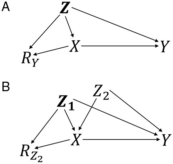
Causal diagrams for missing outcome data (A) and missing confounder data (B). Treatment, $X$; outcome, $Y$; confounders, $Z$, $Z_1$, $Z_2$; indicator of missing outcome data, $R_Y$; indicator of missing confounder $Z_2$ data, $R_{Z_2}$. In Figure 1B, if $Z_2$ is measured prior to assignment/receipt of $X$, the diagram may be altered to include an unmeasured common cause of $X$ and $R_{Z_2}$ without change to assumptions of conditional exchangeability or construction of weights

When outcome data are missing as in Figure 1A, conditioning on the confounders and treatment is required for conditional exchangeability for missingness (i.e. $Y$ and $R_Y$ are d-separated conditional on $\mathit{Z}$ and $X)$ and this exchangeability condition is equivalent to the missing at random (MAR) assumption (conditional on observed data, missingness is independent of unobserved data).²² In this example, the process of estimating formula (1) is straightforward because the variable with missingness, the outcome, is not included in the weight. Recall that the probability of treatment is not conditional on $R_Y=1$ (i.e. the probability of treatment is among all subjects regardless of whether the outcome is observed). Because only the outcome is missing, we can estimate the probability of treatment unconditional on $R_Y=1$ before or after estimating the probability of missingness.

When confounder data are missing as in Figure 1B, $\mathit{Z}$ can be partitioned into fully observed confounders, ${\mathit{Z}}_1$, and a confounder that is not fully observed, $Z_2$; in formula (1), the denominator is now $\mathrm{Pr}\left(R_{Z_2}=1|X=x,{\mathit{Z}}_1,Z_2\right)\mathrm{Pr}\left(X=x|{\mathit{Z}}_1,Z_2\right)$. In the diagram, conditioning on all fully observed confounders and treatment is required for conditional exchangeability for missingness (i.e. $Y$ and $R_{Z_2}$ are d-separated conditional on ${\mathit{Z}}_1$ and $X).\mathrm{ }$Because the variable with missingness, $Z_2$, is included in the weight, estimation is less straightforward than when only outcome data are missing. First, in the missingness probability, we can remove $Z_2$ from the right side of the conditioning bar because $Z_2\coprod R_{Z_2}|X,{\mathit{Z}}_1$, so $\mathrm{Pr}\left(R_{Z_2}=1|X=x,{\mathit{Z}}_1,Z_2\right)=\mathrm{Pr}(R_{Z_2}=1|X=x,{\mathit{Z}}_1)$. This conditional independence ($Z_2\coprod R_{Z_2}|X,{\mathit{Z}}_1$) is a MAR assumption and is an additional condition needed for identification in this example. Second, the treatment probability, $\mathrm{Pr}\left(X=x|{\mathit{Z}}_1,Z_2\right)$, cannot be directly estimated because it is not conditional on $R_{Z_2}=1$ and $Z_2$ is not fully observed. However, this treatment probability can be estimated among the complete cases weighted to correct for missingness, i.e. weighted by the inverse of $\mathrm{Pr}(R_{Z_2}=1|X=x,{\mathit{Z}}_1)$ (see the Supplementary material for proof that relies on the MAR assumption). Therefore, the missingness weights must be estimated prior to estimation of the treatment probabilities. Intuitively, confounder data are missing and we need to recover the distribution of the confounders (using weighting) in order to estimate the treatment probabilities without bias.

If, alternatively, missingness is independent of treatment conditional on confounders (i.e. $X\coprod R|\mathit{Z}$), then the treatment probabilities can be estimated among complete cases because $\mathrm{Pr}\left(X=x|\mathit{Z}\right)=\mathrm{Pr}\left(X=x|R=1,\mathit{Z}\right)$. However, assuming that missingness is independent of treatment is often not appropriate.

Application to simulated data

To illustrate application of the IPW estimator in these examples, we simulated a superpopulation (n = 5 000 000) under the two scenarios depicted in Figure 1 (see the Supplementary material for data generation and code for simulation).

In the first scenario (Figure 1A), missingness of the outcome was caused by a single confounder and treatment. In the second scenario (Figure 1B), missingness of a confounder, $Z_2$, was caused by another confounder$,Z_1$, and treatment, $X$. Treatment and confounders were binary and outcome was continuous. We estimated the weighted marginal counterfactual risks using weights estimated two ways. Approach A used the estimator shown in formula (1). In the example where confounder data were missing, the treatment probabilities were estimated using the missingness weights and then the two weights were combined. In the example where outcome data were missing, the weights were estimated separately and then combined. Approach B used weights constructed as the inverse of the product of the treatment probability conditional on $R=1$ (i.e. estimating the treatment weights among the complete cases) and the missingness probability conditional on $X$ and $Z$, ${\left[\mathrm{Pr}\left(X=x|\mathit{Z},R=1\right)\mathrm{Pr}\left(R=1|X=x,\mathit{Z}\right)\right]}^{-1}$.

Table 1 shows the point estimates of each analysis. We observe that using the weights constructed following formula (1) (approach A) produces consistent estimates. However, estimating the treatment probability among the complete cases (approach B) was biased because treatment was not conditionally independent of missingness. In the absence of careful consideration of formula (1), an investigator may accidentally implement this latter biased approach when confounder data are missing, by estimating the treatment weights without using the missingness weights (see the Supplementary material for proof).

Table 1.

True and estimated marginal expectation of the outcome

				Inverse probability weighted mean
		Truth	Crude	Formula 1a		Treatment probability conditional on $\mathit{R}=1$b
Outcome missingc
Treated ($X=1$)		20.0	24.4	20.0		17.2
Untreated $(X=0$)		20.0	15.7	20.0		22.5
Confounder missingd
Treated ($X=1$)		20.0	16.0	20.0		21.2
Untreated $(X=0$)		20.0	21.8	20.0		18.6

^aWeight when outcome missing: ${\left[\widehat{\mathrm{Pr}}\left(X=x|Z\right)\widehat{\mathrm{Pr}}\left(R=1|X=x,Z\right)\right]}^{-1};\mathrm{ }$weight when confounder ($Z_2$) missing: ${\left[\widehat{\mathrm{Pr}}\left(X=x|Z_1,Z_2\right)\widehat{\mathrm{Pr}}\left(R=1|X=x,Z_1\right)\right]}^{-1}$ where $\widehat{\mathrm{Pr}}\left(X=x|Z_1,Z_2\right)$ was estimated by logistic regression weighted by $\widehat{\mathrm{Pr}}\left(R=1|X=x,Z_1\right)$.

^bWeight when outcome missing:$\mathrm{ }{\left[\widehat{\mathrm{Pr}}\left(X=x|R=1,Z\right)\widehat{\mathrm{Pr}}\left(R=1|X=x,Z\right)\right]}^{-1}$; weight when confounder ($Z_2$) missing: .${\left[\widehat{\mathrm{Pr}}\left(X=x|R=1,Z_1,Z_2\right)\widehat{\mathrm{Pr}}\left(R=1|X=x,Z_1\right)\right]}^{-1}$.

^cCausal diagram Figure 1A.

^dCausal diagram Figure 1B.

Discussion

This work illustrated that IPW can effectively address confounding and missing data biases simultaneously if weights are constructed appropriately. Importantly, we showed that appropriate construction must consider the assumed causal structure and the conditions encoded in the structure that may be leveraged for identification. In the settings examined, the weights could not be constructed using the treatment probabilities estimated from the complete cases. And in the example in which confounder data were missing, estimating the treatment probabilities required use of the missingness weights.

Marginal structural models in longitudinal settings are typically weighted to address confounding and censoring (missing outcome)^1,15 and the treatment weights are usually estimated prior to the censoring weights. Since the treatment probability for the weights does not use outcome data, all individuals are included regardless of censoring status, thus obviating the need to first correct for missingness. However, for our estimand, estimating treatment weights before missingness weights is not valid generally. In the example illustrated above, when confounder data were missing, missingness weights were estimated first and then used in estimation of treatment weights.

For illustration, we have used a simple cohort study design with a time-fixed exposure. The intuition that we need to recover the distribution of missing confounders before estimating treatment weights is applicable to other study designs leveraging IPW, including case-control studies^23,24 and longitudinal studies with time-varying exposures.²⁵ However, the exact form of the estimator and the weights will vary in these settings as the causal structure varies (e.g. outcome directly causes missingness in a case-control setting). Previous work has examined combining weights for missing confounder data and treatments weights in the setting with time-varying treatment.^26,27 However, in most simulated scenarios, treatment and missingness were conditionally independent, thus missingness weights were not needed for estimation of the treatment weights. In real data, it is likely more common that there is missingness in multiple confounders than in a single confounder as in our example. When multiple confounder variables have missingness, the pattern may be uniform, monotone or non-monotone, and the estimation procedure for the missingness weights will vary depending on the pattern.^10,28 Regardless of how the missingness weights are estimated, careful consideration of the causal structure is needed to determine the appropriate form of the estimator and construction of the weights.

This work focuses on the use of weights to address missingness; however, other approaches exist (e.g. multiple imputation) and the choice of a particular approach depends on the specific situation.^{8–10,29–31} A complete case analysis (i.e. dropping records with any missing data) will be unbiased in some settings such as when data are missing completely at random (MCAR), and in even some scenarios when data are MAR or missing not at random (MNAR).^29,32–34 In our examples, consistency of IPW estimates relied on untestable assumptions including conditional exchangeability with positivity, causal consistency, conditional exchangeability for missingness and that data were MAR (these latter two conditions were equivalent when outcome data were missing). However, the conditions for identification are context specific. Sensitivity of conclusions to violations of these assumptions can be explored in quantitative bias analysis or by estimating bounds.^35–37

IPW is an important epidemiological tool that can be used to address systematic biases. When estimating weights, it is important to consider the assumed causal structure, particularly when estimating and combining weights to address multiple biases.

Supplementary data

Supplementary data are available at IJE online.

Funding

R.K.R. was supported by the National Institute on Aging (R01 AG056479) and National Institute of Child Health and Development (T32 HD52468).

Conflict of interest

None declared.

References

- 1. Cole SR, Hernán MA. Constructing inverse probability weights for marginal structural models. Am J Epidemiol 2008;168:656–64. [DOI] [PMC free article] [PubMed] [Google Scholar]
- 2. Horvitz DG, Thompson DJ. A generalization of sampling without replacement from a finite universe. J Am Stat Assoc 1952;47:663–85. [Google Scholar]
- 3. Hernán MA, Robins JM. Estimating causal effects from epidemiological data. J Epidemiol Community Health 2006;60:578–86. [DOI] [PMC free article] [PubMed] [Google Scholar]
- 4. Rogawski ET, Meshnick SR, Becker-Dreps S et al. Reduction in diarrhoeal rates through interventions that prevent unnecessary antibiotic exposure early in life in an observational birth cohort. J Epidemiol Community Health 2016;70:500–05. [DOI] [PMC free article] [PubMed] [Google Scholar]
- 5. Cole SR, Hernán MA. Adjusted survival curves with inverse probability weights. Comput Methods Programs Biomed 2004;75:45–49. [DOI] [PubMed] [Google Scholar]
- 6. Robins JM, Finkelstein DM. Correcting for noncompliance and dependent censoring in an AIDS clinical trial with inverse probability of censoring weighted (IPCW) log-rank tests. Biometrics 2000;56:779–88. [DOI] [PubMed] [Google Scholar]
- 7. Weuve J, Tchetgen Tchetgen EJ, Glymour MM et al. Accounting for bias due to selective attrition; the example of smoking and cognitive decline. Epidemiology 2012;23:119–28. [DOI] [PMC free article] [PubMed] [Google Scholar]
- 8. Seaman SR, White IR. Review of inverse probability weighting for dealing with missing data. Stat Methods Med Res 2013;22:278–95. [DOI] [PubMed] [Google Scholar]
- 9. Perkins NJ, Cole SR, Harel O et al. Principled approaches to missing data in epidemiologic studies. Am J Epidemiol 2018;187:568–75. [DOI] [PMC free article] [PubMed] [Google Scholar]
- 10. Sun BL, Perkins NJ, Cole SR et al. Inverse-probability-weighted estimation for monotone and nonmonotone missing data. Am J Epidemiol 2018;187:585–91. [DOI] [PMC free article] [PubMed] [Google Scholar]
- 11. Cole SR, Stuart EA. Generalizing evidence from randomized clinical trials to target populations, the ACTG 320 trial. Am J Epidemiol 2010;172:107–15. [DOI] [PMC free article] [PubMed] [Google Scholar]
- 12. Westreich D, Edwards JK, Lesko CR, Stuart EA, Cole SR. Transportability of trial results using inverse odds of sampling weights. Am J Epidemiol 2017;186:1010–14. [DOI] [PMC free article] [PubMed] [Google Scholar]
- 13. Lesko CR, Buchanan AL, Westreich D, Edwards JK, Hudgens MG, Cole SR. Generalizing study results: a potential outcomes perspective. Epidemiology 2017;28:553–61. [DOI] [PMC free article] [PubMed] [Google Scholar]
- 14. Westreich D. Epidemiology by Design: A Causal Approach to the Health Sciences. New York, NY: Oxford University Press, 2020. [Google Scholar]
- 15. Hernán MA, Brumback B, Robins JM. Marginal structural models to estimate the causal effect of zidovudine on the survival of HIV-positive men . Epidemiology 2000;11:561–70. [DOI] [PubMed] [Google Scholar]
- 16. Little RJ, Rubin DB. Causal effects in clinical and epidemiological studies via potential outcomes: concepts and analytical approaches. Annu Rev Public Health 2000;21:121–45. [DOI] [PubMed] [Google Scholar]
- 17. Pearl J. Causal inference in statistics: an overview. Stat Surv 2009;3:96–146. [Google Scholar]
- 18. Westreich D, Cole SR. Invited commentary: positivity in practice. Am J Epidemiol 2010;171:674–77. [DOI] [PMC free article] [PubMed] [Google Scholar]
- 19. Cole SR, Frangakis CE. The consistency statement in causal inference: a definition or an assumption? Epidemiology 2009;20:3–5. [DOI] [PubMed] [Google Scholar]
- 20. Mohan K, Pearl J. Graphical models for processing missing data. J Am Stat Assoc 2021;116:1023–37. [Google Scholar]
- 21. Hernán MA, Robins JM. Causal Inference: What If. Boca Raton, FL: Chapman & Hall/CRC, 2020. [Google Scholar]
- 22. Little RJA, Rubin DB. Statistical Analysis with Missing Data. 2nd edn. Hoboken, NJ: Wiley, 2002. [Google Scholar]
- 23. Lee H, Hudgens MG, Cai J, Cole SR. Marginal structural Cox models with case-cohort sampling. Stat Sin 2016;26:509–26. [DOI] [PMC free article] [PubMed] [Google Scholar]
- 24. Cole SR, Hudgens MG, Tien PC et al. Marginal structural models for case-cohort study designs to estimate the association of antiretroviral therapy initiation with incident AIDS or death. Am J Epidemiol 2012;175:381–90. [DOI] [PMC free article] [PubMed] [Google Scholar]
- 25. Robins JM, Hernán MA. Estimation of the causal effects of time-varying exposures. In: Fitzmaurice G, Davidian M, Verbeke G, Molenbergsh G (eds). Longitudinal Data Analysis. Boca Raton, FL: Chapman & Hall/CRC, 2008, pp. 553–97. [Google Scholar]
- 26. Moodie EEM, Delaney JAC, Lefebvre G, Platt RW. Missing confounding data in marginal structural models: a comparison of inverse probability weighting and multiple imputation. Int J Biostat 2008;4:Article 13. [DOI] [PubMed] [Google Scholar]
- 27. Vourli G, Touloumi G. Performance of the marginal structural models under various scenarios of incomplete marker’s values: a simulation study. Biom J 2015;57:254–70. [DOI] [PubMed] [Google Scholar]
- 28. Sun BL, Tchetgen Tchetgen EJ. On inverse probability weighting for nonmonotone missing at random data. J Am Stat Assoc 2018;113:369–79. [DOI] [PMC free article] [PubMed] [Google Scholar]
- 29. Bartlett JW, Harel O, Carpenter JR. Asymptotically unbiased estimation of exposure odds ratios in complete records logistic regression. Am J Epidemiol 2015;182:730–36. [DOI] [PMC free article] [PubMed] [Google Scholar]
- 30. Harel O, Mitchell EM, Perkins NJ et al. Multiple imputation for incomplete data in epidemiological studies. Am J Epidemiol 2018;187:576–84. [DOI] [PMC free article] [PubMed] [Google Scholar]
- 31. Seaman SR, White IR, Copas AJ, Li L. Combining multiple imputation and inverse-probability weighting. Biometrics 2012;68:129–37. [DOI] [PMC free article] [PubMed] [Google Scholar]
- 32. Daniel RM, Kenward MG, Cousens SN, De Stavola BL. Using causal diagrams to guide analysis in missing data problems. Stat Methods Med Res 2012;21:243–56. [DOI] [PubMed] [Google Scholar]
- 33. Ross RK, Breskin A, Westreich D. When is a complete-case approach to missing data valid? The importance of effect-measure modification. Am J Epidemiol 2020;189:1583–89. [DOI] [PMC free article] [PubMed] [Google Scholar]
- 34. Westreich D. Berksons bias, selection bias, and missing data. Epidemiology 2012;23:159–64. [DOI] [PMC free article] [PubMed] [Google Scholar]
- 35. Lash TL, Fox MP, Fink AK. Applying Quantitative Bias Analysis to Epidemiological Data. New York, NY: Springer, 2009. [Google Scholar]
- 36. Lash TL, Fox MP, Maclehose RF, Maldonado G, Mccandless LC, Greenland S. Good practices for quantitative bias analysis. Int J Epidemiol 2014;43:1969–85. [DOI] [PubMed] [Google Scholar]
- 37. Breskin A, Westreich D, Cole SR, Edwards JK. Using bounds to compare the strength of exchangeability assumptions for internal and external validity. Am J Epidemiol 2019;188:1355–60. [DOI] [PMC free article] [PubMed] [Google Scholar]
Associated Data
This section collects any data citations, data availability statements, or supplementary materials included in this article.