Abstract
Cement production is one of the most energy-intensive manufacturing industries, and the milling circuit of cement plants consumes around 4% of a year's global electrical energy production. It is well understood that modeling and digitalizing industrial-scale processes would help control production circuits better, improve efficiency, enhance personal training systems, and decrease plants' energy consumption. This tactical approach could be integrated using conscious lab (CL) as an innovative concept in the internet age. Surprisingly, no CL has been reported for the milling circuit of a cement plant. A robust CL interconnect datasets originated from monitoring operational variables in the plants and translating them to human basis information using explainable artificial intelligence (EAI) models. By initiating a CL for an industrial cement vertical roller mill (VRM), this study conducted a novel strategy to explore relationships between VRM monitored operational variables and their representative energy consumption factors (output temperature and motor power). Using SHapley Additive exPlanations (SHAP) as one of the most recent EAI models accurately helped fill the lack of information about correlations within VRM variables. SHAP analyses highlighted that working pressure and input gas rate with positive relationships are the key factors influencing energy consumption. eXtreme Gradient Boosting (XGBoost) as a powerful predictive tool could accurately model energy representative factors by R-square ever 0.80 in the testing phase. Comparison assessments indicated that SHAP-XGBoost could provide higher accuracy for VRM-CL structure than conventional modeling tools (Pearson correlation, Random Forest, and Support vector regression.
Subject terms: Energy science and technology, Engineering
Introduction
As one of the most energy-intensive industries, cement plants consume around 100 kWh of electrical energy for each ton of their production. This can be counted yearly as over 6% of global energy consumption. More than 60% of this tremendous energy has been used in the comminution units (crushers and mills) to reduce the size of raw materials and clinker1–3. In the mid-1990s, the vertical roller mill (VRM) was introduced to the cement industry to reduce this energy usage. Besides lowering power consumption, VRMs may improve process capacity and simplify it since VRMs can simultaneously implement milling and drying processes. However, controlling VRM performances and understanding relationships within their operational variables need serious attention4–7.
In the cement plant, the conventional VRM controlling systems mainly rely on the field staff to manually adjust the few process parameters based on their experience. These adjustments generally lead to having an unstable system, increasing power consumption, and reducing plant productivity8. For filling these gaps and having a long-term stable operation, it would be essential to provide a complete picture of relationships within VRM elements. Understanding these correlations and their magnitude would help develop models for generating robust controlling systems. Generating such systems and assessing the VRM process operational parameters would help to optimize power consumption, improve maintenance, reduce environmental issues, and make the process sustainable.
A few investigations have been conducted to model VRM performance. Fernandes et al.9 used the back-propagation neural network (BPNN) to model size products of a raw VRM mill. They indicated RMSprop as an optimizer for modeling raw meal residual values would generate a lower error than the Adagrad and Adam optimizers. Their results showed that BPNN algorithms could accurately predict raw meal residue product quality in the cement industry. The population balance model for simulation of a VRM in a cement clinker grinding circuit was investigated by Fatahi and Barani11. They reported that the clinker particle spent a short time inside the VRM, and the mean residence time is about 67 s. The tanks-in series model compared to the Weller model was more proper to describe the residence time distributions in the VRM11. Extreme learning as an artificial intelligence (AI) method was used for modeling online measurement quality parameters of a raw material VRM. Results showed that the proposed model effectively achieved the online estimation of the key indicator parameters for the VRM process, laying the foundation for online parameter optimization11. However, no published study has been modeled and examined inter-correlations between VRM energy consumption indicative factors and plant operational parameters. Using “conscious lab (CL)” and constructing models based on operational data originated from industrial VRM could be an innovative way to tackle these gaps.
CL as a new model vision constructs based on datasets that have been generated by monitoring operational parameters within industrial plants12–15. CL is exploring relationships between these parameters by using AI systems and highlighting the effectiveness of each variable on the key process factors16,17. CL can be upgraded using explainable artificial intelligence (EAI) models as an innovative concept. EAI systems are emerging approaches of modeling that translate big complicated datasets into know-how information and relieve considerable transparency by converting complex relationships into human basis structures18,19. In other words, EAIs can change black box AI systems into white-box ones. CL constructed using EAI models and real processing datasets can be a powerful tool for ranking operational variables based on their importance, reducing time, cost, and possible laboratory and scale-up errors, and can be considered for training operating person based on the plant reality.
As a strategic approach, for the first time, this investigation is going to develop a CL based on over 3000 records monitored from a cement VRM circuit by using the most recent generated EAI models called "SHAP" (SHapley Additive exPlanations). Based on the game-theoretic approach, SHAP explores relationships within variables (linearly and nonlinearly), ranks them based on their importance, and marks their magnitude. SHAP illustrates these correlations for every record of variables and develops a complete explanation between the global average and the model output20–23. Besides SHAP, a sophisticated CL system would be required to predict the output variables accurately. Thus, XGBoost (eXtreme Gradient Boosting), a comprehensive predictive tool, has been employed to model motor power and outlet temperature as representative energy consumption factors of the VRM circuit. XGBoost is a flexible AI predictor tool with high performance and accuracy22,24–27. One of the main advantages of XGBoost over other typical machine learning methods is its more significant set of hyperparameters, which makes it capable of being better tuned. For comparison purposes, random forest28–31 and support vector regression32–35 as conventional AI methods have also been used to assess the SHAP-XGBoost ability to develop CL of VRM.
Materials and methods
Database
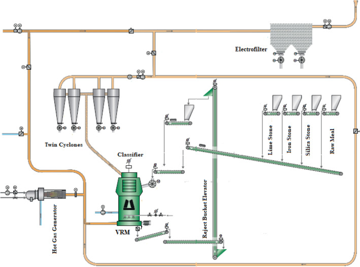
The provided data were collected from a cement plant (Fig. 1) located in Ilam, west of Iran. The plant has two cement production lines which in total produces 5300 t/day cement. The raw materials (lime, silica, and iron ore) enter the circuit through two apron feeders. The raw materials are crushed in a hammer crusher to D95 80 mm. The raw materials were mixed in a certain proportion and fed into a vertical roller mill (LOESCHE mill). The raw vertical roller mill has four rollers, 3000 KW main drive, 4.8 m table diameter, 2.16 m roller diameter with 330 t/h capacity (made by LOESCHE Company from Germany). The table mill's rotation speeds are mainly constant, and there is approximately a fixed one-year period of changing liners of the mill body and hardfacing operations of wear rollers. For constructing a CL dedicated to the VRM circuit and predicting motor power and outlet temperature (as indicative energy factors), a dataset was collected from one of the vertical roller raw mill circuits (line 2) in the Ilam cement plant. The critical operating parameters gathered during the standard operation are summarized in Table 1. Variables were monitored hourly and were taken into account. In general, over 3000 records were prepared and used for the modeling.
Figure 1.
Schematic of raw vertical roller mill circuit in the Ilam cement plant.
Table 1.
Monitoring variables in the Ilam cement plant (STD: Standard deviation).
| Description of variables | Variables | Min | Max | Mean | STD |
|---|---|---|---|---|---|
| The load of mill feed | Feed rate (ton/h) | 250 | 307 | 297.16 | 7.11 |
| The applied pressure for grinding by roller | Working pressure (bar) | 68 | 80 | 72.76 | 1.92 |
| The required hot gas for drying and transportation of raw material | Input gas flow (m3/h) | 60,000 | 890,000 | 600,559 | 90,434 |
| The speed of classifiers rotor | Classifier speed (rpm) | 48 | 59 | 52.47 | 1.03 |
| The vibration of mill body due to operational parameters | Mill body vibrating (mm/s) | 2.30 | 36.90 | 4.16 | 1.13 |
| The temperature of the mill inlet | Input temperature (°C) | 21 | 2132 | 204.50 | 61.26 |
| The differential pressure between inlet and outlet of mill | ΔP (mbar) | 9 | 97 | 85.37 | 3.45 |
| The pressure of the mill inlet | Input pressure (mbar) | − 6 | 4 | − 2.27 | 0.88 |
| The temperature of the mill outlet | Output temperature (°C) | 7 | 98 | 66.99 | 9.82 |
| The power drawing of the main motor | Motor power (kW) | 138 | 2370 | 1845.76 | 397.32 |
In the LOESCHE mill, the rollers are hydraulically pressed against a disc table, and the feed would be crushed and pulverized between the rollers and the disc table. The motor power running all four rollers was calculated based on Eq. (1). In other words, the rollers are hydraulically pressed by working pressure against a table, and the feed is ground between the rollers and the table36–38. Therefore, working pressure would affect the size distribution of products. The main motor power is related to the rollers' applied pressure (working pressure) and the feed rate of raw materials on the grinding table. The hot gas was produced by kiln and preheater7. For drying, ground materials are transported to the separator by hot gas that is introduced into the mill. Thus, the difference between the input and output pressures of the mill (ΔP) would be essential. Dried material will be transferred for size classification37. Unground material would stay over the classifier, and they have to be kept inside the mill to meet the desired size. One of the critical factors through the process is controlling the mill body vibrating as a result of the working pressure of the rollers on the crushing table39. After the grinding, drying, transportation, and separation process inside the mill, the product is transferred as cement kiln feed to a storage silo.
| 1 |
where Cos (Cos is 0.88 for the Ilam cement production) is the power factor, I is the current, V is the voltage, and P is the power.
Modeling
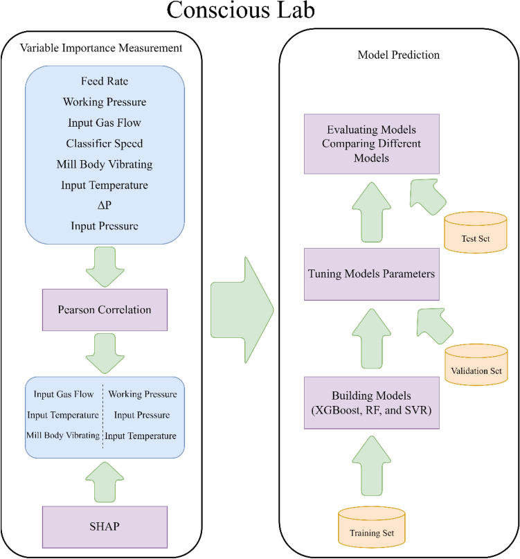
After removing the missing data, the provided dataset was processed by different AI models. SHAP and Pearson correlation were initially considered to assess the relationship between variables. After that, the dataset was randomly split into three sections: training (70%), validation (15%), and testing (15%). Similar dataset sections were considered for constructing all the proposed models for comparison purposes. The procedure was based on the following diagram (Fig. 2).
Figure 2.
Constructing a conscious lab for a vertical roller mill.
SHapley Additive exPlanations (SHAP)
SHAP stands for "SHapley Additive exPlanations", a machine learning (ML) approach to explain models predictions and provide interpretability of an ML model. First presented by Lloyd Shapley, it uses Shapley values to interpret the model's output16,23,40,41. The Shapley value of a feature is equal to the difference between the average prediction value of samples with and without this feature42. It measures the feature's importance in the model43,44. Shapley value for the model can be computed as follows:
| 2 |
where represents the set of all input variables, denotes a subset of with the th feature excluded from , and is the marginal feature contribution of the th variable45–48.
Extreme Gradient Boosting (XGBoost)
Extreme Gradient Boosting (XGBoost), proposed by Chen and Guestrin49, is an efficient and scalable ensemble algorithm based on gradient boosted trees16,50. XGBoost has been used in a wide range of engineering fields, resulting in outstanding performance due to the advantages of parallel tree boosting and using various regularization techniques13,51,52. XGBoost is a stable algorithm with low bias and variance, handling outliers24,53. It adds a regularization term to the objective function as follows:
| 3 |
where is a convex loss function and is a regularization function used to avoid overfitting by controlling the model's complexity54. is calculated as follows:
| 4 |
where denotes the number of leaf nodes, and is the weight of each leaf. and are regularization parameters that determine the relative weight of each penalty term24,55–57.
Random forest
Random forest (RF) is an ensemble learning technique that combines the bagged integrated learning theory58 with the random subspace approach59,60. RF is a nonparametric method, robust to outliers, and can handle missing values in data16,61,62. RF is a collection of decision trees that are grown independently. The predictions of these trees are aggregated by averaging to generate the final output. This ensures that the overall variance is reduced24,56,63. Mathematically speaking, RF generates an ensemble of decision trees. Using these trees, the final output of an input feature vector is computed as follows:
| 5 |
Support vector regression
Support vector regression (SVR) is a nonparametric supervised machine learning approach proposed by Drucker67. Vapnik's support vector concept was the inspiration for Drucker to develop SVR67. An important feature of SVR is its powerful capability for nonlinear predictions68, which results from the nonlinear transformation it uses. SVR maps observations into a higher-dimensional feature space via nonlinear transformation and then solves the problem24,69,70. Given a training dataset with samples , , , the following linear function can formulate non-linear relation between input and output:
| 6 |
where denotes the estimated output and is a mapping function. and (i.e., bias) are two parameters that can be determined by optimizing the following objective function:
| 7 |
where is the penalty parameter or regularization constant, and denote slack variables that represent the upper and lower constraints on the output variable13,24,71–73.
Evaluation
Coefficient of determination (R2), Root mean square error (RMSE), and the differences between actual and predicted values in different stages of modeling (training, validating, and testing) were used to assess the model's accuracy.
| 8 |
where denotes the sum of squares of residuals and is the total sum of squares that can be computed as follows:
| 9 |
where and represent the observed data and mean of the observed data, respectively. RMSE can be calculated as follows:
| 10 |
where and denote the predicted and observed values, respectively, and represents the number of samples. Moreover, to assess whether the performance of the XGBoost is statistically significant, a two-tailed Welch’s t-test with a significance level was applied for RMSE and R2 between the XGBoost and other methods, and the obtained p-value was reported. Welch’s t-test is a nonparametric univariate statistical test used to test the hypothesis that two samples have equal means74.
Results and discussions
Relationship assessments
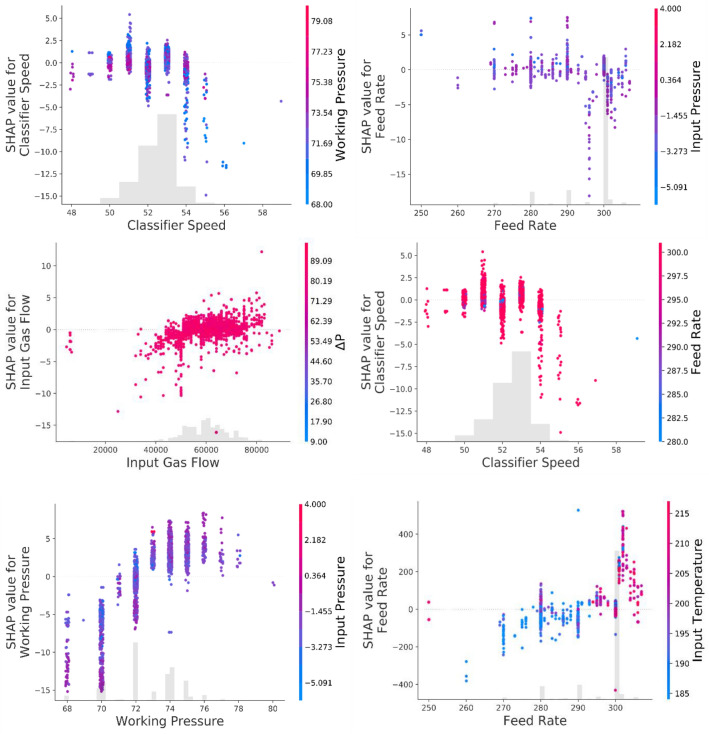
Exploring correlations and ranking variables based on their effectiveness on key parameters would help operate heavy machines such as VRMs accurately, make the process sustainable and reduce energy consumption. For drawing insights about relationships with the VRM variables, Pearson correlation (as a typical correlation assessment method) and SHAP assessment were conducted through the entire recorded data from the plant. SHAP (Fig. 3) showed the complexity of relationships between VRM operational variables. Ranking variables (Figs. 4, 5) based on their importance (SHAP values) illustrated that working pressure and input gas flow had the highest effectiveness on output temperature and motor power, respectively. Their correlations were positive. Working pressure (grinding pressure) could be considered the most effective variable through the VRM size reduction process. Increasing working pressure enhances the energy applied to the material, and more fines are offered to the classifier, leaving the circuit faster37. Altun et al.6 indicated a strong correlation coefficient between and product rate. In other words, increasing the work pressure would enhance energy consumption6,7,37,75.
Figure 3.
SHAP assessed the complexity of inter-correlations between VRM operational variables.
Figure 4.
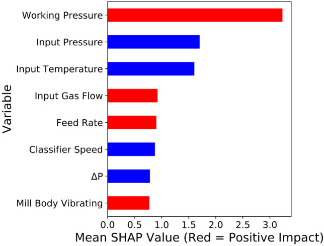
Ranking SHAP values and magnitude of relationships between VRM monitoring variables and output temperature.
Figure 5.
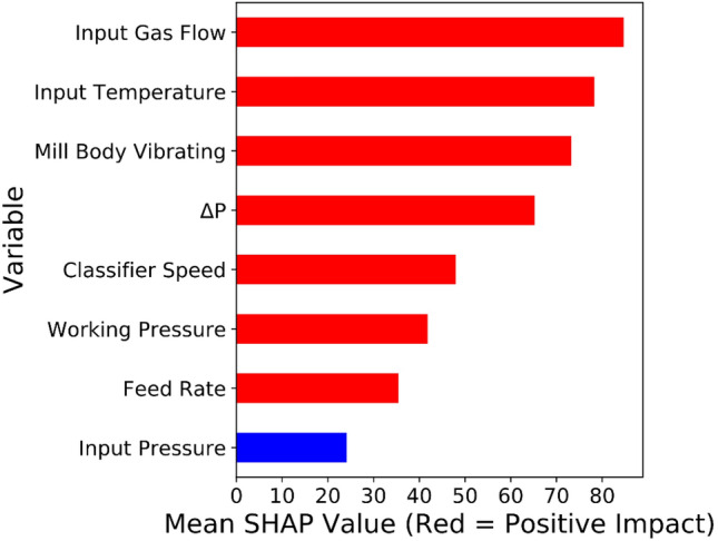
Ranking SHAP values and magnitude of relationships between VRM monitoring variables and motor power.
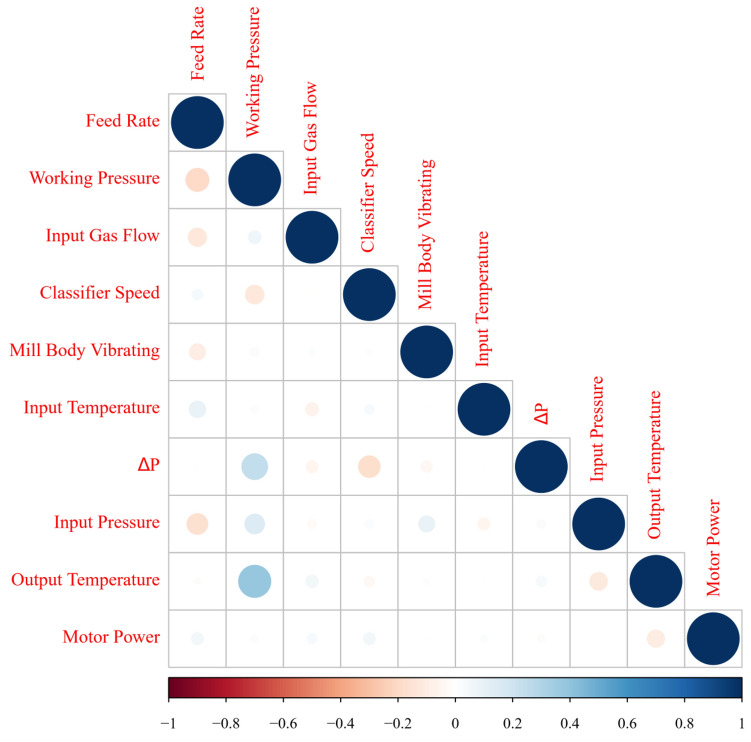
There is a good agreement between SHAP and Pearson correlation outcomes (Fig. 6); however, SHAP could model relationships much more accurately. It was well documented that Pearson correlation can only examine one by one linear relationship and show their magnitude. While, SHAP would develop a multi-linear-nonlinear interaction assessment among the recorded variables, rank them based on their importance, and highlight the magnitude of the multivariable relationships. For example, while linear relationship examination by Pearson correlation showed no significant interactions between input pressure or temperature and VRM indicative energy consumption factors, SHAP placed it within the most influential variables. Obviously, input temperature would affect the output temperature of products. Moreover, input pressure could commendably affect the process energy consumption since too low negative inlet pressure influences the steady gas flow within the system and disturbs the grinding procedure6,37,75. Pearson correlation showed a positive relationship between motor power, while multivariable assessment by SHAP illustrated a negative correlation. VRMs are very prone to vibration if their operational variables marginally are varied. It was reported that slight vibration could enhance particle transportation and improve energy consumption7. Apart from linear assessment (Fig. 5), gas flow also influences energy consumption factors, as SHAP illustrated (Fig. 4). Gas flow through the mill helps ensure constant lift for the internal circulating material and keeps separator performance constant to ensure a consistent product size distribution6,76.
Figure 6.
Pearson correlation assessments between VRM monitoring variables.
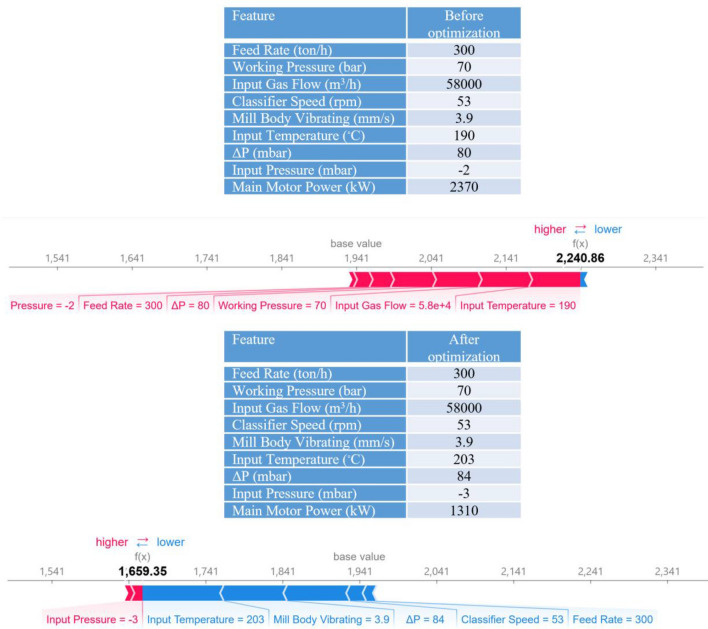
It was reported that only the mill input material feed rate has a decisive influence on the mill differential pressure (ΔP) while gas flow rate, grinding pressure, and classifier speed are maintained at the similar condition according to the pre-adjustments during operation unless the characteristics of the raw material such as the grind ability of the material have been changed6,76. However, SHAP results showed by increasing the ΔP, the power consumption was increased (Fig. 4). This correlation can be explained by the fact that variations in the ΔP when the grinding pressure and the hot air circulation are constant directly reflect the amount of material inside the mill. In other words, when the ΔP decreases, the amount of input material is less than the discharge material, causing the material bed to be thinner. Thus, as the ΔP increases, the material bed becomes thicker. VRM vibrates when the material bed is too thin or thick and trips or stops when the vibration limit is exceeded. For these reasons, the total feed amount must be adjusted so that the ΔP is within the correct range6,76. Based on these facts, SHAP analyses indicated (Fig. 7) that keeping the most effective parameter constant and changing other variables for the same size production makes it possible to reduce energy consumption. These results demonstrated that CL can model motor power and output temperature.
Figure 7.
Possible optimization for the motor power consumption based on the SHAP results.
Predictive models
For constructing predictive AI models (XGBoost, RF, and SVR), from the entire provided dataset, 70% of records were randomly used for the training step, 15% for the validation and the rest were considered for the testing step. Many XGBoost features were explored and adjusted during the training step for finding the most accurate models and tuning process (Table 2). The XGBoost validation and testing stage outcomes (Table 3) demonstrated that the generated model could quite accurately predict the energy consumption indicative essential factors based on the plant monitored variables. A comparison between various models' outcomes (Table 3) highlighted that the XGBoost model resulted in higher accuracy than these two conventional AI models for the prediction (Fig. 8). A two-tailed Welch’s t-test with a significance level was applied for R2 and RMSE between the XGBoost and other methods, and the obtained p-value was reported in Table 3. As can be seen, in all comparisons, the null hypothesis is rejected based on the statistical tests with a 95% confidence level, and the results are considered statistically significant.
Table 2.
The XGBoost parameter settings for predicting VRM indicative energy parameters.
| Parameter | Value (output temperature) | Value (motor power) |
|---|---|---|
| Base learner | Gradient boosted tree | Gradient boosted tree |
| Tree construction algorithm | Exact greedy | Exact greedy |
| Learning objective | Regression with squared loss | Regression with squared loss |
| Learning rate () | 0.260 | 0.225 |
| Lagrange multiplier () | 6.53 | 1 |
| Number of gradients boosted trees | 60 | 81 |
| Maximum depth of trees | 16 | 7 |
| The minimum sum of instance weight (Hessian) needed in a child | 1 | 1 |
| L2 regularization term on weights | 1 | 1 |
| The initial prediction score of all instances (global bias) | 0.5 | 0.5 |
| Subsample ratio of the training instances | 1 | 1 |
| Maximum delta step, we allow each leaf output to be | 0 (there is no constraint) | 0 (there is no constraint) |
Table 3.
Outcomes of various models in the validation and testing stages.
| Method | Output temperature | |||||
|---|---|---|---|---|---|---|
| R2 | RMSE | |||||
| Validation | Test | p-value | Validation | Test | p-value | |
| Random forest | ||||||
| Avg | 0.88 | 0.83 | 3.69E − 09 | 2.42 | 2.56 | 6.58E − 14 |
| std | (0.02) | (0.07) | (0.19) | (0.50) | ||
| Support vector regression | 0.49 | 0.39 | 1.82E − 168 | 4.88 | 4.94 | 3.78E − 185 |
| XGBoost | 0.99 | 0.99 | – | 0.36 | 0.41 | – |
| Motor power | ||||||
|---|---|---|---|---|---|---|
| Random forest | ||||||
| Avg | 0.71 | 0.62 | 1.53E − 25 | 186.11 | 217.65 | 3.30E − 25 |
| std | (0.01) | (0.01) | (2.54) | (3.59) | ||
| Support vector regression | 0.17 | 0.19 | 1.33E − 168 | 313.47 | 313.22 | 1.95E − 214 |
| XGBoost | 0.80 | 0.80 | – | 151.66 | 155.60 | – |
Figure 8.
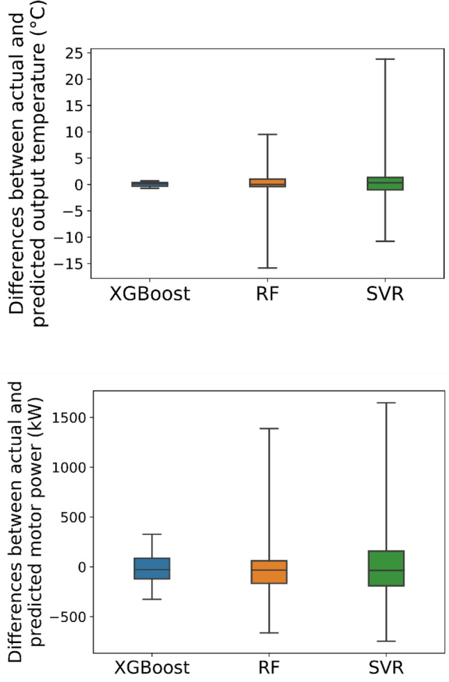
Differences between actual and predicted energy consumption indicative variables generated by various models in the testing phase.
By comparing different machine learning methods used in this research, it is crucial noting that RF and XGBoost are both ensemble techniques, whereas SVR is not. XGBoost is a boosting method that builds on weak learners to train the next learner to enhance the already trained ensemble. RF is a bagging method that uses a random subset of features to train each weak learner independently. XGBoost and SVR have a low computational cost, but RF does not. SVR takes advantage of the kernel trick, and XGBoost uses parallel processing to reduce the computational cost. All three methods are getting little impact from outliers. XGBoost and RF are performed well with missing data in the dataset, but SVR does not. SVR has low bias and high variance in terms of bias and variance, while XGBoost and RF have low bias and variance24,53,77–80. These outcomes illustrated that SHAP-XGBoost could effectively construct a CL for a VRM circuit as an impressive EAI structure. Moreover, these results showed that using EAI can highlight the reality of relationships between operating variables on the industrial scale. Therefore, besides controlling the system regarding the process variables, it would be possible to predict the performance of existing machines based on the new feed materials, reduce penalties and keep the circuit sustainable. The robust capability of such a system depicted the potential of industrial digitalization for understanding, predicting, and maintaining various powder technology processes and controlling their energy consumption.
Conclusion
Understanding relationships among operational variables can effectively help to improve control systems and reduce energy consumption in the cement plant as one of the most intensive energy consumer industries. Digitalization and constructing a conscious lab for exploring correlations between operational variables of a vertical roller mill and its indicative energy factors would potentially enhance its maintenance and efficiency. SHAP-XGBoost, as one of the most recently developed explainable artificial intelligence systems, would be a novel approach for developing a conscious lab and converting industrial datasets to understandable human basis pictures. SHAP-XGBoost could accurately depict correlations among operational parameters of an industrial vertical roller mill. SHAP assessment indicated that working pressure and input gas flow had the highest effectiveness (positive correlations) on output temperature and motor power, respectively. Pearson correlation and SHAP could highlight a negative inter-correlation between classifier speed and working pressure. Moreover, results showed that increasing the input gas flow would decrease the input temperature. XGBoost has accurately estimated the vertical roller mill's output temperature and motor power based on the plant monitoring variables (R-square over 0.99, and 0.80 for the output temperature and motor power, respectively). In the validation and testing stages, a comparison between results of SHAP-XGBoost and the other examined conventional models (Pearson correlation, random forest, and support vector regression) indicated that SHAP-XGBoost as a powerful method could be applied for generating conscious labs which dedicated to the energy sector factors within powder production technologies.
Author contributions
S.C.C. and H.N.: Conceptualization, methodology, software, validation, formal analysis, investigation, writing—original draft, writing—review and editing. E.D. and R.F.: Conceptualization, methodology, validation, formal analysis, resources.
Data availability
The dataset used to support the findings of this study is available from the corresponding author upon request.
Competing interests
The authors declare no competing interests.
Footnotes
Publisher's note
Springer Nature remains neutral with regard to jurisdictional claims in published maps and institutional affiliations.
Contributor Information
Hamid Nasiri, Email: h.nasiri@aut.ac.ir.
Saeed Chehreh Chelgani, Email: saeed.chelgani@ltu.se.
References
- 1.Atmaca A, Kanoglu M. Reducing energy consumption of a raw mill in cement industry. Energy. 2012;42:261–269. doi: 10.1016/j.energy.2012.03.060. [DOI] [Google Scholar]
- 2.Cantini A, et al. Technological energy efficiency improvements in cement industries. Sustainability. 2021;13:3810. doi: 10.3390/su13073810. [DOI] [Google Scholar]
- 3.Kermeli K, et al. The scope for better industry representation in long-term energy models: Modeling the cement industry. Appl. Energy. 2019;240:964–985. doi: 10.1016/j.apenergy.2019.01.252. [DOI] [Google Scholar]
- 4.Schaefer HU. Loesche vertical roller mills for the comminution of ores and minerals. Miner. Eng. 2001;14:1155–1160. doi: 10.1016/S0892-6875(01)00133-9. [DOI] [Google Scholar]
- 5.Reichert M, Gerold C, Fredriksson A, Adolfsson G, Lieberwirth H. Research of iron ore grinding in a vertical-roller-mill. Miner. Eng. 2015;73:109–115. doi: 10.1016/j.mineng.2014.07.021. [DOI] [Google Scholar]
- 6.Altun D, Benzer H, Aydogan N, Gerold C. Operational parameters affecting the vertical roller mill performance. Miner. Eng. 2017;103:67–71. doi: 10.1016/j.mineng.2016.08.015. [DOI] [Google Scholar]
- 7.Pareek P, Sankhla VS. Review on vertical roller mill in cement industry and its performance parameters. Mater. Today Proc. 2021;44:4621–4627. doi: 10.1016/j.matpr.2020.10.916. [DOI] [Google Scholar]
- 8.Meng, Q., Wang, Y., Xu, F. & Shi, X. Control strategy of cement mill based on bang-bang and fuzzy PID self-tuning. in 2015 IEEE International Conference on Cyber Technology in Automation, Control, and Intelligent Systems (CYBER) 1977–1981 (2015).
- 9.Fernandes, H., Halim, A. & Wahab, W. Modeling Vertical Roller Mill Raw Meal Residue by Implementing Neural Network. in 2019 IEEE International Conference on Innovative Research and Development (ICIRD) 1–6 (2019).
- 10.Fatahi R, Barani K. Modeling and simulation of vertical roller mill using population balance model. Physicochem. Probl. Miner. Process. 2020;56(01):24–33. [Google Scholar]
- 11.Lin, X. & Liang, J. Modeling based on the extreme learning machine for raw cement mill grinding process. in Proceedings of the 2015 Chinese Intelligent Automation Conference 129–138 (2015).
- 12.Tohry A, Yazdani S, Hadavandi E, Mahmudzadeh E, Chelgani SC. Advanced modeling of HPGR power consumption based on operational parameters by BNN: A “Conscious-Lab” development. Powder Technol. 2021;381:280–284. doi: 10.1016/j.powtec.2020.12.018. [DOI] [Google Scholar]
- 13.Chehreh Chelgani S, Nasiri H, Tohry A. Modeling of particle sizes for industrial HPGR products by a unique explainable AI tool—A “Conscious Lab” development. Adv. Powder Technol. 2021;32:4141–4148. doi: 10.1016/j.apt.2021.09.020. [DOI] [Google Scholar]
- 14.Alidokht M, Yazdani S, Hadavandi E, Chelgani SC. Modeling metallurgical responses of coal Tri-Flo separators by a novel BNN: A “Conscious-Lab” development. Int. J. Coal Sci. Technol. 2021;8(6):1436–1446. doi: 10.1007/s40789-021-00423-7. [DOI] [Google Scholar]
- 15.Chelgani SC, Jorjani E. Artificial neural network prediction of Al2O3 leaching recovery in the Bayer process—Jajarm alumina plant (Iran) Hydrometallurgy. 2009;97:105–110. doi: 10.1016/j.hydromet.2009.01.008. [DOI] [Google Scholar]
- 16.Chelgani SC, Nasiri H, Alidokht M. Interpretable modeling of metallurgical responses for an industrial coal column flotation circuit by XGBoost and SHAP—A “conscious-lab” development. Int. J. Min. Sci. Technol. 2021;31:1135–1144. doi: 10.1016/j.ijmst.2021.10.006. [DOI] [Google Scholar]
- 17.Fatahi R, et al. Ventilation prediction for an Industrial Cement Raw Ball Mill by BNN—A “Conscious Lab” approach. Materials (Basel). 2021;14:3220. doi: 10.3390/ma14123220. [DOI] [PMC free article] [PubMed] [Google Scholar]
- 18.Chakraborty D, et al. Scenario-based prediction of climate change impacts on building cooling energy consumption with explainable artificial intelligence. Appl. Energy. 2021;291:116807. doi: 10.1016/j.apenergy.2021.116807. [DOI] [Google Scholar]
- 19.Akhlaghi YG, et al. Hourly performance forecast of a dew point cooler using explainable Artificial Intelligence and evolutionary optimisations by 2050. Appl. Energy. 2021;281:116062. doi: 10.1016/j.apenergy.2020.116062. [DOI] [Google Scholar]
- 20.Chelgani SC. Estimation of gross calorific value based on coal analysis using an explainable artificial intelligence. Mach. Learn. with Appl. 2021;6:100116. doi: 10.1016/j.mlwa.2021.100116. [DOI] [Google Scholar]
- 21.Manojlović V, Kamberović Ž, Korać M, Dotlić M. Machine learning analysis of electric arc furnace process for the evaluation of energy efficiency parameters. Appl. Energy. 2022;307:118209. doi: 10.1016/j.apenergy.2021.118209. [DOI] [Google Scholar]
- 22.Feng Y, Duan Q, Chen X, Yakkali SS, Wang J. Space cooling energy usage prediction based on utility data for residential buildings using machine learning methods. Appl. Energy. 2021;291:116814. doi: 10.1016/j.apenergy.2021.116814. [DOI] [Google Scholar]
- 23.Wen X, Xie Y, Wu L, Jiang L. Quantifying and comparing the effects of key risk factors on various types of roadway segment crashes with LightGBM and SHAP. Accid. Anal. Prev. 2021;159:106261. doi: 10.1016/j.aap.2021.106261. [DOI] [PubMed] [Google Scholar]
- 24.Nasiri H, Homafar A, Chehreh Chelgani S. Prediction of uniaxial compressive strength and modulus of elasticity for Travertine samples using an explainable artificial intelligence. Results Geophys. Sci. 2021;8:100034. [Google Scholar]
- 25.Patnaik B, Mishra M, Bansal RC, Jena RK. MODWT-XGBoost based smart energy solution for fault detection and classification in a smart microgrid. Appl. Energy. 2021;285:116457. doi: 10.1016/j.apenergy.2021.116457. [DOI] [Google Scholar]
- 26.Wang Z, Hong T, Piette MA. Building thermal load prediction through shallow machine learning and deep learning. Appl. Energy. 2020;263:114683. doi: 10.1016/j.apenergy.2020.114683. [DOI] [Google Scholar]
- 27.Alsahaf A, Petkov N, Shenoy V, Azzopardi G. A framework for feature selection through boosting. Expert Syst. Appl. 2022;187:115895. doi: 10.1016/j.eswa.2021.115895. [DOI] [Google Scholar]
- 28.Shahbazi B, Chelgani SC, Matin SS. Prediction of froth flotation responses based on various conditioning parameters by Random Forest method. Colloids Surfaces A Physicochem. Eng. Asp. 2017;529:936–941. doi: 10.1016/j.colsurfa.2017.07.013. [DOI] [Google Scholar]
- 29.Nazari S, et al. Flotation of coarse particles by hydrodynamic cavitation generated in the presence of conventional reagents. Sep. Purif. Technol. 2019;220:61–68. doi: 10.1016/j.seppur.2019.03.033. [DOI] [Google Scholar]
- 30.Tohry A, Chelgani SC, Matin SS, Noormohammadi M. Power-draw prediction by random forest based on operating parameters for an industrial ball mill. Adv. Powder Technol. 2020;31:967–972. doi: 10.1016/j.apt.2019.12.012. [DOI] [Google Scholar]
- 31.Chelgani SC, Matin SS. Study the relationship between coal properties with Gieseler plasticity parameters by random forest. Int. J. Oil Gas Coal Technol. 2018;17:113–127. doi: 10.1504/IJOGCT.2018.089345. [DOI] [Google Scholar]
- 32.Chelgani SC, Shahbazi B, Hadavandi E. Support vector regression modeling of coal flotation based on variable importance measurements by mutual information method. Measurement. 2018;114:102–108. doi: 10.1016/j.measurement.2017.09.025. [DOI] [Google Scholar]
- 33.Hadavandi E, Hower JC, Chelgani SC. Modeling of gross calorific value based on coal properties by support vector regression method. Model. Earth Syst. Environ. 2017;3:1–7. doi: 10.1007/s40808-017-0270-7. [DOI] [Google Scholar]
- 34.Hadavandi E, Chelgani SC. Estimation of coking indexes based on parental coal properties by variable importance measurement and boosted-support vector regression method. Measurement. 2019;135:306–311. doi: 10.1016/j.measurement.2018.11.068. [DOI] [Google Scholar]
- 35.Chelgani SC, Hadavandi E, Hower JC. Study relationship between the coal thermoplastic factor with its organic and inorganic properties by the support vector regression method. Int. J. Coal Prep. Util. 2020;40:743–754. doi: 10.1080/19392699.2017.1409215. [DOI] [Google Scholar]
- 36.Chatterjee AK. Cement Production Technology: Principles and Practice. CRC Press; 2018. [Google Scholar]
- 37.Altun D. Mathematical Modelling of Vertical Roller Mills. Fen Bilimleri Enstitüsü; 2017. [Google Scholar]
- 38.Simmons M, Gorby L, Terembula J. Operational experience from the United States’ first vertical roller mill for cement grinding. Conf. Rec. Cement Ind. Tech. Conf. 2005;2005:241–249. [Google Scholar]
- 39.Pareek P, Sankhla VS. Increase productivity of vertical roller mill using seven QC tools. IOP Conf. Series Mater. Sci. Eng. 2021;1017:12035. doi: 10.1088/1757-899X/1017/1/012035. [DOI] [Google Scholar]
- 40.Mao H, et al. Driving safety assessment for ride-hailing drivers. Accid. Anal. Prev. 2021;149:105574. doi: 10.1016/j.aap.2020.105574. [DOI] [PubMed] [Google Scholar]
- 41.Mangalathu S, Shin H, Choi E, Jeon J-S. Explainable machine learning models for punching shear strength estimation of flat slabs without transverse reinforcement. J. Build. Eng. 2021;39:102300. doi: 10.1016/j.jobe.2021.102300. [DOI] [Google Scholar]
- 42.Liang M, et al. Interpretable Ensemble-Machine-Learning models for predicting creep behavior of concrete. Cem. Concr. Compos. 2022;125:104295. doi: 10.1016/j.cemconcomp.2021.104295. [DOI] [Google Scholar]
- 43.Jones EJ, et al. Identifying causes of crop yield variability with interpretive machine learning. Comput. Electron. Agric. 2022;192:106632. doi: 10.1016/j.compag.2021.106632. [DOI] [Google Scholar]
- 44.Zheng X, et al. Using machine learning to predict atrial fibrillation diagnosed after ischemic stroke. Int. J. Cardiol. 2022;347:21–27. doi: 10.1016/j.ijcard.2021.11.005. [DOI] [PubMed] [Google Scholar]
- 45.Wang D, et al. Towards better process management in wastewater treatment plants: Process analytics based on SHAP values for tree-based machine learning methods. J. Environ. Manage. 2022;301:113941. doi: 10.1016/j.jenvman.2021.113941. [DOI] [PubMed] [Google Scholar]
- 46.Bussmann N, Giudici P, Marinelli D, Papenbrock J. Explainable machine learning in credit risk management. Comput. Econ. 2021;57:203–216. doi: 10.1007/s10614-020-10042-0. [DOI] [Google Scholar]
- 47.García MV, Aznarte JL. Shapley additive explanations for NO2 forecasting. Ecol. Inform. 2020;56:101039. doi: 10.1016/j.ecoinf.2019.101039. [DOI] [Google Scholar]
- 48.Adland R, Jia H, Lode T, Skontorp J. The value of meteorological data in marine risk assessment. Reliab. Eng. Syst. Saf. 2021;209:107480. doi: 10.1016/j.ress.2021.107480. [DOI] [Google Scholar]
- 49.Chen, T. & Guestrin, C. Xgboost: A scalable tree boosting system. in Proceedings of the 22nd ACM SIGKDD International Conference on Knowledge Discovery and Data Mining 785–794 (2016).
- 50.Yun KK, Yoon SW, Won D. Prediction of stock price direction using a hybrid GA-XGBoost algorithm with a three-stage feature engineering process. Expert Syst. Appl. 2021;186:115716. doi: 10.1016/j.eswa.2021.115716. [DOI] [Google Scholar]
- 51.Shehadeh A, Alshboul O, Al Mamlook RE, Hamedat O. Machine learning models for predicting the residual value of heavy construction equipment: An evaluation of modified decision tree, LightGBM, and XGBoost regression. Autom. Constr. 2021;129:103827. doi: 10.1016/j.autcon.2021.103827. [DOI] [Google Scholar]
- 52.Nasiri H, Alavi SA. A novel framework based on deep learning and ANOVA feature selection method for diagnosis of COVID-19 cases from chest X-ray images. Comput. Intell. Neurosci. 2022;2022:4694567. doi: 10.1155/2022/4694567. [DOI] [PMC free article] [PubMed] [Google Scholar]
- 53.Huang J-C, et al. Predictive modeling of blood pressure during hemodialysis: A comparison of linear model, random forest, support vector regression, XGBoost, LASSO regression and ensemble method. Comput. Methods Programs Biomed. 2020;195:105536. doi: 10.1016/j.cmpb.2020.105536. [DOI] [PubMed] [Google Scholar]
- 54.Hasani S, Nasiri H. COV-ADSX: An automated detection system using X-ray images, deep learning, and XGBoost for COVID-19. Softw. Impacts. 2022;11:100210. doi: 10.1016/j.simpa.2021.100210. [DOI] [PMC free article] [PubMed] [Google Scholar]
- 55.Jiang, F. et al. An aging-aware soc estimation method for lithium-ion batteries using xgboost algorithm. in 2019 IEEE International Conference on Prognostics and Health Management (ICPHM) 1–8 (2019).
- 56.Zhang W, Wu C, Zhong H, Li Y, Wang L. Prediction of undrained shear strength using extreme gradient boosting and random forest based on Bayesian optimization. Geosci. Front. 2021;12:469–477. doi: 10.1016/j.gsf.2020.03.007. [DOI] [Google Scholar]
- 57.Nasiri H, Hasani S. Automated detection of COVID-19 cases from chest X-ray images using deep neural network and XGBoost. Radiography. 2022 doi: 10.1016/j.radi.2022.03.011. [DOI] [PMC free article] [PubMed] [Google Scholar]
- 58.Kwok SW, Carter C. Multiple decision trees. In: Shachter RD, Levitt TS, Kanal LN, Lemmer JF, editors. Machine Intelligence and Pattern Recognition. Elsevier; 1990. pp. 327–335. [Google Scholar]
- 59.Ho TK. The random subspace method for constructing decision forests. IEEE Trans. Pattern Anal. Mach. Intell. 1998;20:832–844. doi: 10.1109/34.709601. [DOI] [Google Scholar]
- 60.Liu Z, Shi Y. A hybrid IDS using GA-based feature selection method and random forest. Int. J. Mach. Learn. Comput. 2022;12(02):43–50. [Google Scholar]
- 61.Hou S, Liu Y, Yang Q. Real-time prediction of rock mass classification based on TBM operation big data and stacking technique of ensemble learning. J. Rock Mech. Geotech. Eng. 2022;14(01):123–143. doi: 10.1016/j.jrmge.2021.05.004. [DOI] [Google Scholar]
- 62.Srinivasan S, et al. Physics-informed machine learning for backbone identification in discrete fracture networks. Comput. Geosci. 2020;24:1429–1444. doi: 10.1007/s10596-020-09962-5. [DOI] [Google Scholar]
- 63.Carranza C, Nolet C, Pezij M, Van Der Ploeg M. Root zone soil moisture estimation with Random Forest. J. Hydrol. 2021;593:125840. doi: 10.1016/j.jhydrol.2020.125840. [DOI] [Google Scholar]
- 64.Abellán-García J, Guzmán-Guzmán JS. Random forest-based optimization of UHPFRC under ductility requirements for seismic retrofitting applications. Constr. Build. Mater. 2021;285:122869. doi: 10.1016/j.conbuildmat.2021.122869. [DOI] [Google Scholar]
- 65.Zhou J, et al. Random forests and cubist algorithms for predicting shear strengths of rockfill materials. Appl. Sci. 2019;9:1621. doi: 10.3390/app9081621. [DOI] [Google Scholar]
- 66.Jafrasteh B, Fathianpour N, Suárez A. Comparison of machine learning methods for copper ore grade estimation. Comput. Geosci. 2018;22:1371–1388. doi: 10.1007/s10596-018-9758-0. [DOI] [Google Scholar]
- 67.Drucker H, et al. Support vector regression machines. Adv. Neural Inf. Process. Syst. 1997;9:155–161. [Google Scholar]
- 68.Tang R, Fan C, Zeng F, Feng W. Data-driven model predictive control for power demand management and fast demand response of commercial buildings using support vector regression. Build. Simul. 2022;15:317–331. doi: 10.1007/s12273-021-0811-x. [DOI] [Google Scholar]
- 69.Roy A, Chakraborty S. Reliability analysis of structures by a three-stage sequential sampling based adaptive support vector regression model. Reliab. Eng. Syst. Saf. 2022;219:108260. doi: 10.1016/j.ress.2021.108260. [DOI] [Google Scholar]
- 70.Miranda T, Sousa LR, Gomes AT, Tinoco J, Ferreira C. Geomechanical characterization of volcanic rocks using empirical systems and data mining techniques. J. Rock Mech. Geotech. Eng. 2018;10:138–150. doi: 10.1016/j.jrmge.2017.11.003. [DOI] [Google Scholar]
- 71.He J, Mattis SA, Butler TD, Dawson CN. Data-driven uncertainty quantification for predictive flow and transport modeling using support vector machines. Comput. Geosci. 2019;23:631–645. doi: 10.1007/s10596-018-9762-4. [DOI] [Google Scholar]
- 72.Paryani S, Neshat A, Pourghasemi HR, Ntona MM, Kazakis N. A novel hybrid of support vector regression and metaheuristic algorithms for groundwater spring potential mapping. Sci. Total Environ. 2022;807:151055. doi: 10.1016/j.scitotenv.2021.151055. [DOI] [PubMed] [Google Scholar]
- 73.Wei J, Dong G, Chen Z. Remaining useful life prediction and state of health diagnosis for lithium-ion batteries using particle filter and support vector regression. IEEE Trans. Ind. Electron. 2018;65:5634–5643. doi: 10.1109/TIE.2017.2782224. [DOI] [Google Scholar]
- 74.Haeri MA, Ebadzadeh MM, Folino G. Improving GP generalization: A variance-based layered learning approach. Genet. Program. Evolvable Mach. 2015;16:27–55. doi: 10.1007/s10710-014-9220-6. [DOI] [Google Scholar]
- 75.Joergensen, S. W. Cement grinding vertical roller mills versus ball mills. in 13th Arab-International Cement Conference and Exhibition 26 (2004).
- 76.Yan-yan, N., Guang, Z., Ming-zhe, Y. & Zhuo, W. Design of intelligent control system for Vertical Roller Mill. in 2011 2nd International Conference on Intelligent Control and Information Processing1, 315–318 (2011).
- 77.Harode B, Jain A. Adaptive approaches for IDS: A review. Int. J. Res. Anal. Rev. 2018;5:361–363. [Google Scholar]
- 78.Boccard J, Rudaz S. Mass spectrometry metabolomic data handling for biomarker discovery. In: Issaq HJ, Levitt TD, editors. Proteomic and Metabolomic Approaches to Biomarker Discoveryn. Elsevier; 2013. pp. 425–445. [Google Scholar]
- 79.Fan J, et al. Comparison of Support Vector Machine and Extreme Gradient Boosting for predicting daily global solar radiation using temperature and precipitation in humid subtropical climates: A case study in China. Energy Convers. Manag. 2018;164:102–111. doi: 10.1016/j.enconman.2018.02.087. [DOI] [Google Scholar]
- 80.Lee Y, Han D, Ahn M-H, Im J, Lee SJ. Retrieval of total precipitable water from Himawari-8 AHI data: A comparison of random forest, extreme gradient boosting, and deep neural network. Remote Sens. 2019;11:1741. doi: 10.3390/rs11151741. [DOI] [Google Scholar]
Associated Data
This section collects any data citations, data availability statements, or supplementary materials included in this article.
Data Availability Statement
The dataset used to support the findings of this study is available from the corresponding author upon request.


