Nationwide and Regional PM_2.5‐Related Air Quality Health Benefits From the Removal of Energy‐Related Emissions in the United States

Abstract

Clean energy policy can provide substantial health benefits through improved air quality. As ambitious clean energy proposals are increasingly considered and adopted across the United States (US), quantifying the benefits of removal of such large air pollution emissions sources is crucial to understanding potential societal impacts of such policy. In this study, we estimate health benefits resulting from the elimination of emissions of fine particulate matter (PM_2.5), sulfur dioxide, and nitrogen oxides from the electric power, transportation, building, and industrial sectors in the contiguous US. We use EPA's CO‐Benefits Risk Assessment screening tool to estimate health benefits resulting from the removal of PM_2.5‐related emissions from these energy‐related sectors. We find that nationwide efforts to eliminate energy‐related emissions could prevent 53,200 (95% CI: 46,900–59,400) premature deaths each year and provide $608 billion ($537–$678 billion) in benefits from avoided PM_2.5‐related illness and death. We also find that an average of 69% (range: 32%–95%) of the health benefits from emissions removal remain in the emitting region. Our study provides an indication of the potential scale and distribution of public health benefits that could result from ambitious regional and nationwide clean energy and climate mitigation policy.

Key Points

• Eliminating air pollutant emissions from energy‐related sectors could prevent more than 50,000 deaths each year in the United States

• The elimination of these emissions sources would provide over $600 billion in health benefits from avoided death and illness each year

• Much of the benefit from removing emissions remains in the region where emissions were removed, indicating local benefits of local action

1. Introduction

There is a clean energy transition underway in the United States (US). Since 2015, about a dozen states and the District of Columbia (DC) and Puerto Rico have set targets requiring that all their electricity production come from clean or carbon‐free sources, in many cases by between 2040 and 2050, and other states have set similar non‐binding goals (Paulos et al., 2021). Such ambitious clean energy proposals are most common in the electric power sector, but others focus on transportation. In 2020, California set a goal through executive action requiring that all new passenger vehicles sold by 2035 be zero‐emission (California Executive Order N‐79‐20, 2020). Some pledges are even starting to extend to the whole of the economy. Governors in California, Louisiana, and Michigan have issued executive orders calling for economy‐wide carbon neutrality, and in 2021 Massachusetts became the first state to pass legislation aimed at reaching net‐zero GHG emissions statewide (Paulos et al., 2021). There is also renewed interest in climate and clean energy policy at the federal level. The Biden administration has called for 100% carbon‐free electricity nationwide by 2035, a 50%–52% reduction from 2005 levels in economy‐wide GHG emissions by 2030, and net‐zero emissions economy‐wide by no later than 2050 (The White House, 2021).

Despite these promising goals, the current pace of decarbonization in the US is still incompatible with a world in which global warming is limited to 1.5°C or 2°C above preindustrial levels, the targets set in the Paris Agreement (United Nations Environment Programme, 2020). Climate change poses health risks ranging from increases in heatwave mortality and vector‐ and water‐borne diseases to respiratory illness from allergens and wildfires, injuries and mental health stress from flooding and storms, and malnutrition and population displacement from severe drought (Patz et al., 2014). Deep and rapid cuts in GHG emissions are needed in all energy‐related sectors—including electric power, transportation, buildings, and industry—if states and the country as a whole are to achieve reductions consistent with avoiding the worst impacts of climate change (Intergovernmental Panel on Climate Change, 2018).

Many of the same activities and processes that emit planet‐warming GHGs also release health‐harming air pollutant emissions; the current air quality‐related health burden associated with fossil fuels is substantial. Fossil fuel combustion is a significant source of particulate matter (PM) pollution (Klimont et al., 2017; Weagle et al., 2018). Exposure to ambient fine PM_2.5 pollution is among the largest environmental risk factors for disease in the US and is associated with premature mortality from chronic obstructive pulmonary disease (COPD); lower respiratory infections (LRIs); tracheal, bronchus, and lung cancer; diabetes; ischemic heart disease (IHD); and stroke (Institute for Health Metrics and Evaluation, 2022). Ambient PM_2.5 exposure from all sources led to 131,000 premature deaths in the US in 2015 (Tessum et al., 2019), though other studies that use updated evidence of the association between PM_2.5 exposure and mortality suggest the toll may be as high as 283,000 (Lelieveld et al., 2019).

Transitioning energy production away from fossil fuels and toward cleaner sources can produce health benefits from improved air quality in the near term while also providing climate benefits in the longer term (Haines & Ebi, 2019; Patz et al., 2020). Cost‐effectiveness and cost‐benefit analyses increasingly include estimates of health benefits of clean energy policy proposals (Grab et al., 2019). Studies of the air quality health benefits of climate and clean energy policy tend to focus on the electric power and transportation sectors (Gallagher & Holloway, 2020). Many previous studies have shown the substantial health benefits of expanding renewable energy production in the US (Barbose et al., 2016; Buonocore et al., 2016, 2019; Dimanchev et al., 2019; McCubbin & Sovacool, 2013; Millstein et al., 2017; Wiser et al., 2016). Barbose et al. (2016) estimate that reductions in emissions of PM_2.5, sulfur dioxide (SO₂), and nitrogen oxides (NO_x) resulting from the deployment of renewable energy capacity to replace fossil fuel electricity generation in 2013 and meet targets set by state renewable portfolio standards provided $2.6–$9.9 billion (2013 dollars) in health benefits from avoided premature mortality and morbidity, including non‐fatal heart attacks and work loss days. Millstein et al. (2017) found that US wind and solar deployment from 2007 to 2015 resulted in a cumulative $29.7–$112.8 billion (2015 dollars) in air‐quality benefits and prevented 3,000–12,700 premature deaths because of reduced PM_2.5, SO₂, and NO_x emissions.

The relative contribution of nearby and distant emissions sources to health harms can differ by pollutant type and emissions source. Previous work has estimated health harms attributable to air pollution emissions from distant and out‐of‐state sources (Dedoussi et al., 2020; Goodkind et al., 2019; Penn et al., 2017; Sergi et al., 2020). Goodkind et al. (2019), for example, found that 33% of monetized health damages resulting from the emission of primary PM_2.5, SO₂, NO_x, ammonia (NH₃), and volatile organic compounds in the contiguous US in 2011 occurred within 8 km of an emission source but 25% occurred more than 256 km downwind of a source. Dedoussi et al. (2020) found that 41%–53% of the PM_2.5‐ and ozone‐related premature mortality from a state's combustion emissions from 2005 to 2018 occurred outside the emitting state. Similarly, Sergi et al. (2020) found that about 70% of health damages from PM_2.5 exposure in the US in 2008, 2011, and 2014 were due to emissions from counties other than the county in which damages occurred and 32% were due to emissions from states other than the state in which damages occurred in 2014.

Research on the regional and interstate transport of air pollution and associated health effects can provide useful information for decision makers given existing regulatory frameworks and organizational structures. The National Ambient Air Quality Standards (NAAQS), set by the US Environmental Protection Agency (EPA), limit the allowable ambient concentration of six criteria air pollutants—including PM (i.e., PM_2.5 and coarse PM₁₀), SO₂, and nitrogen dioxide (NO₂)—with primary standards intended to protect human health (U.S. EPA, 2021c). The “good neighbor” provision of the Clean Air Act requires that states consider the effect of their emissions on the ability of downwind states to satisfy the NAAQS (U.S. EPA, 2022b). The Cross‐State Air Pollution Rule requires that 27 states reduce emissions from fossil fuel–fired electricity generating units (EGUs) to help downwind areas meet PM_2.5 and/or ozone NAAQS (U.S. EPA, 2022c). Much of the work of EPA is executed by its 10 regional offices, each of which serves several states and territories (U.S. EPA, 2021f), and there are regional organizations that facilitate collaboration on air quality issues at regional scales (U.S. EPA, 2021g).

In this study, we provide an assessment of the health benefits of the elimination of PM_2.5‐related emissions in the US energy system. We calculate avoided air pollution damages that would result from the elimination of primary PM_2.5, SO₂, and NO_x emissions from six energy‐related sectors: electricity fuel use, residential/commercial fuel use, industrial fuel use, on‐road vehicles, non‐road vehicles, and oil and gas production and refining. While emissions in these sectors are predominantly the result of fossil fuel use, a substantial portion of primary PM_2.5 emissions comes from wood and bark burning in residential and industrial settings and a small portion comes from non‐combustion sources. Ambient PM_2.5 concentration changes and associated health benefits are measured using the US EPA's CO‐Benefits Risk Assessment (COBRA) screening tool (U.S. EPA, 2021b). Though our analysis includes no energy system modeling, our results provide a suggestion of the scale of annual benefits that could result from a strict zero‐emission energy system decarbonization scenario. The sectors analyzed here constitute nearly 90% of 2016 US CO₂‐equivalent GHG emissions (U.S. EPA, 2022a). Our analysis also presents a novel use of COBRA for understanding the regional and interstate transfer of air‐quality health benefits from emissions reductions in energy‐related sectors. We report the portion of health benefits resulting from emissions removal in an EPA region that would accrue in the source region and all other regions (U.S. EPA, 2021f).

Quantifying the air‐quality health benefits of emissions reductions can be time‐ and resource‐intensive, often requiring the use of sophisticated analytic methods (Fann et al., 2012; U.S. EPA, 2020). However, reduced‐complexity models (RCMs) like COBRA have been shown to reliably reproduce results from “state‐of‐the‐science” chemical transport models (CTMs) and can be useful in initial research and policy scoping (Gilmore et al., 2019; Industrial Economics, Inc., 2019). RCMs commonly used in the literature include the Estimating Air pollution Social Impact Using Regression (EASIUR) model, Intervention Model for Air Pollution (InMAP), and Air Pollution Emissions Experiments and Policy (APEEP), the last of which has the same core air‐quality modeling framework as COBRA (Gilmore et al., 2019). In a report prepared for the EPA, researchers found that AP3, a version of APEEP, provided nationwide estimates of avoided PM_2.5‐related mortality that were 1.0 and 1.1 those produced by the Comprehensive Air Quality Model with Extensions (CAMx) combined with the Environmental Benefits Mapping and Analysis Program (BenMAP) for a modeled emissions scenario of the Clean Power Plan (Industrial Economics, Inc., 2019). AP3 performed worse when estimating avoided mortality from an emissions scenario of the Tier 3 Emission and Fuel Standard, reporting totals that were 2.7 and 4.3 times those from CAMx with BenMAP (Industrial Economics, Inc., 2019). While CTMs are more suitable for use in cost‐effectiveness and cost‐benefit analysis, RCMs can offer insight into the benefits of policies at the early stages of development and are generally practicable by a wide user base, including legislators, public health officials, and civil society groups. The use of COBRA in this analysis also allows us to model emissions changes and associated health benefits for many more regions and sectors than would be practical using a CTM.

2. Materials and Methods

Avoidable PM_2.5‐related health burdens are estimated based on reduced emissions of primary PM_2.5, SO₂, and NO_x. This framework uses a reduced‐complexity air quality and health impact modeling tool to provide comparable and rapid order‐of‐magnitude estimates of benefits that would be useful during the early stages of policy development. Limitations and advantages of reduced‐form modeling are outlined in the Discussion. All dollar amounts are listed in 2020 US dollars unless otherwise noted. All calculations are performed with unrounded estimates.

2.1. Air Quality Modeling

We use version 4.0 of EPA's COBRA screening tool to estimate ambient PM_2.5 concentration changes resulting from the removal of PM_2.5, SO₂, and NO_x emissions in energy‐related sectors in the US (U.S. EPA, 2021b). We use default 2016 model year parameters for baseline emissions and for the source‐receptor (S‐R) matrix and adjustment factors. Baseline county‐level emissions are derived from 2016 base year emissions inventory compiled by the 2016v1 Emissions Modeling Platform, a product of the National Emissions Inventory (NEI) Collaborative (National Emissions Inventory Collaborative, 2019).

COBRA uses the Phase II S‐R Matrix, which estimates the contribution of primary PM_2.5 and its precursors, including SO₂ and NO_x (which can form secondary PM_2.5 upon release into the atmosphere), from each emission source to annual average PM_2.5 concentrations. Emissions from ground‐level mobile and area sources, as well as elevated point sources with effective stack heights of 0–500 m, are modeled as originating from a hypothetical source at the county centroid, and elevated point sources with effective stack heights greater than 500 m use true latitude and longitude coordinates (U.S. EPA, 2020). The S‐R matrix is based on the Climatological Regional Dispersion Model, which includes terms for wet and dry deposition of primary and secondary PM_2.5 species and uses annual average mixing heights and joint frequency distributions of wind speed and direction based on 1990 meteorology data. COBRA estimates the transport of directly emitted PM_2.5 and secondary organic aerosols, SO₂, NO₂, and NH₃. For each of these pollutant types, a matrix of S‐R transfer coefficients was developed for each unique combination of source and receptor sites (i.e., counties) in the contiguous US. Chemical conversion of secondary species is assumed to occur at the receptor site. The S‐R matrix provides representative estimates of changes in ambient PM_2.5 concentrations resulting from increases or decreases in emissions, but it does not fully account for atmospheric transport mechanisms or nonlinearities in atmospheric chemistry that lead to secondary PM_2.5 formation (e.g., SO₂‐to‐sulfate and NO_x‐to‐nitrate chemistry). COBRA returns a point estimate of PM_2.5 for each county, so it is not possible to determine the contribution of speciated PM_2.5 components to overall concentrations, at least with available model outputs.

We model emissions removal for six energy‐related Tier 1 emissions categories: electric utility fuel combustion, industrial fuel combustion, other fuel combustion, highway vehicles, off‐highway, and petroleum and related industries. For ease of understanding, we refer to these emissions sectors as such: electric utility fuel combustion as “electricity fuel use,” industrial fuel combustion as “industrial fuel use,” other fuel combustion as “residential/commercial fuel use,” highway vehicles as “on‐road vehicles,” off‐highway as “non‐road vehicles,” and petroleum and related industries as “oil and gas production and refining.” The Tier 2 and 3 emissions sources included in each of these six Tier 1 categories are listed in Table S1 in Supporting Information S1. We estimate that the vast majority of SO₂ (94%) and NO_x (95%) emissions and about half (51%) of primary PM_2.5 emissions in these sectors are from fossil fuel use. Almost the entirety of the remainder of primary PM_2.5 emissions are the result of residential wood burning (34%) and the combustion of wood/bark waste by industry (12%).

Some emissions sources included in these sectors are not strictly related to energy production and use. For example, asphalt manufacturing comprises 8%, 3%, and 0.5% of primary PM_2.5, SO₂, and NO_x emissions from oil and gas production and refining (0.21%, 0.11%, and 0.03% from all six Tier 1 sectors). Non‐exhaust vehicle PM_2.5 emissions from brake wear and tire wear, which would not be abated in a shift to zero‐emission vehicles, cannot be disaggregated from total vehicle emissions in the COBRA emissions profile. The inclusion of these sources in our analysis means that results for on‐ and non‐road vehicles are likely an overestimate. For calendar year 2016, brake wear and tire wear from light‐duty gasoline and diesel vehicles emitted roughly similar amounts of PM_2.5 as vehicle exhaust on a per‐mile basis, slightly less from motorcycles and light‐duty gasoline trucks, and much less from light‐duty diesel trucks and heavy‐duty diesel vehicles (Bureau of Transportation Statistics, 2021). That said, NO_x emissions from vehicle exhaust still contribute relatively more to PM_2.5‐related health burdens than primary PM_2.5 emissions from transportation, whether from vehicle exhaust or brake wear and tire wear (Choma et al., 2021; Goodkind et al., 2019). PM_2.5 emissions from the suspension of dust from paved and unpaved roads are included in another source category in the emissions inventory and do not affect our results.

For each model run, we zero out (i.e., reduce by 100%) emissions of primary PM_2.5, SO₂, and NO_x from the relevant sectors. We model nationwide (i.e., 48 contiguous states and DC) emissions removal for all sectors simultaneously, then nationwide emissions removal for each sector independently, and finally statewide emissions removal for all sectors simultaneously. We report uncertainty in our mortality estimates as the 95% confidence intervals of the standard error of the mean beta coefficients used in the health impact modeling. This approach does not characterize uncertainty from other sources, most notably the choice of value of a statistical life (VSL), which other studies have shown to be the largest potential source of uncertainty in monetized estimates (Goodkind et al., 2019). Since COBRA returns point estimates for modeled PM_2.5 concentration changes, we cannot determine uncertainty resulting from the air quality modeling.

For validation, we evaluate how well COBRA reproduces observed concentrations by comparing baseline COBRA PM_2.5 concentrations to 2016 county‐level annual average PM_2.5 monitor data from the EPA Air Quality System (U.S. EPA, 2021e). Relevant data are for parameter code 88101 (i.e., “PM_2.5–Local Conditions”) and metric used “Daily Mean.” Duplicate values are removed. For counties with multiple monitor sites or measurement instruments, we average reported values to create a single estimate for each county.

2.2. Health Impact Modeling

We run COBRA using default health impact functions for all morbidity and mortality endpoints. The health impact modeling component of COBRA relies on evidence from the epidemiological literature about the relationship between PM_2.5 exposure and adverse health effects. This information is combined with county‐level population counts and baseline incidence rates for health effects including premature all‐cause mortality, infant mortality, non‐fatal heart attacks, and respiratory hospital admissions (U.S. EPA, 2020). For some health outcomes, such as asthma exacerbation, prevalence data are used in place of incidence data.

We calculate avoided premature mortality using four concentration‐response functions (CRFs). The first two CRFs, from PM_2.5–mortality relationships described by Krewski et al. (2009) and Lepeule et al. (2012), are the default mortality functions included in COBRA. They rely on evidence from follow‐ups of the American Cancer Society (ACS) and Harvard Six Cities studies, respectively, long‐term US cohort studies of air pollution exposure. These studies found relative risks of all‐cause mortality of 1.06 (95% CI: 1.04–1.08) and 1.14 (95% CI: 1.07–1.22), respectively, for a 10 μg/m³ increase in PM_2.5. (Findings from epidemiological studies, often reported as relative risk for a specific change in PM_2.5 [e.g., 10 or 20 μg/m³], are used to calculate coefficients that can be used to estimate health effects for any change in concentration.) The third CRF, the Global Exposure Mortality Model (GEMM) reported by Burnett et al. (2018), relies on data from 41 cohort studies from 16 countries to estimate the shape of the association between ambient PM_2.5 exposure and non‐accidental mortality. The GEMM function is supralinear at lower concentrations, near‐linear at higher concentrations, and applies a counterfactual threshold of 2.4 μg/m³, the lowest concentration observed in any of the cohort studies. It is assumed that PM_2.5 exposure has no effect on health below this level. The fourth CRF is from Tessum et al. (2019) and is based on the relationship described by Nasari et al. (2016) and Burnett et al. (2018) but is derived from the ACS cohort instead of the full list of 41 cohorts.

Following COBRA model runs, we apply the GEMM function to outputted county‐level changes in PM_2.5 concentrations. We report estimates of mortality using the GEMM function as our central estimate and include results from COBRA's default mortality functions as sensitivities. The CRF described by Tessum et al. (2019) is also included as a sensitivity and to allow for comparison to other work, which is further detailed in Section 2.4. The fraction of deaths attributable to a given PM_2.5 exposure level for the mortality functions used in this study are shown in Figure S1 in Supporting Information S1.

The GEMM function produces mortality estimates that are much higher than those from the Integrated Exposure Response (IER) model used in Global Burden of Disease studies (Burnett et al., 2018; Hystad et al., 2020). The IER function reports mortality attributable to five causes of death: IHD, stroke, COPD, lung cancer, and LRIs (Cohen et al., 2017). Burnett et al. (2018) provide versions of the GEMM function that estimate mortality from these same causes of death (i.e., GEMM 5‐COD), but the primary GEMM function estimates non‐accidental mortality (i.e., noncommunicable diseases [NCDs] and LRIs, abbreviated as GEMM NCD + LRI). Hystad et al. (2020) argue that the use of the GEMM function for global disease burden estimation warrants caution since much of the global population is exposed to PM_2.5 concentrations above the ranges observed in the cohort studies that inform the GEMM function, but we consider it an appropriate choice for this analysis since the US is well represented in PM_2.5 cohort studies included in the GEMM function.

We use the primary GEMM NCD + LRI function since this produces mortality estimates more similar to those from the default mortality functions in COBRA, which estimate all‐cause mortality, than would cause‐specific functions. There are versions of the GEMM function that are parameterized differently depending on whether the function is segmented by age and whether a cohort of Chinese men with a wider PM_2.5 exposure range than the other studies is included. The version we use applies a single function to estimates of non‐accidental mortality for all ages >25 and includes the Chinese male cohort. This function takes the form:

$$\mathrm{H}\mathrm{R}\left(\mathsf{x}\right)=e^{0.143\left(\frac{\ln \left(\frac{\max (0,\mathsf{x}-2.4)}{1.6}+1\right)}{1+e^{\frac{-\max (0,\mathsf{x}-2.4)-15.5}{36.8}}}\right)}$$

where $\mathrm{H}\mathrm{R}\left(\mathsf{x}\right)$ is the hazard ratio of mortality incidence at PM_2.5 concentration $\mathsf{x}$. The attributable fraction (AF) of deaths from PM_2.5 exposure is then calculated as:

$$\mathrm{A}\mathrm{F}=\frac{\mathrm{H}\mathrm{R}\left(\mathsf{x}\right)-1}{\mathrm{H}\mathrm{R}\left(\mathsf{x}\right)}$$

The number of deaths for a given PM_2.5 concentration is then estimated by:

$$M=\mathrm{A}\mathrm{F}·y·\mathrm{p}\mathrm{o}\mathrm{p}$$

where M is the number of deaths, y is the non‐accidental mortality rate, and pop is the population count. We then calculate the number of deaths that could be avoided by eliminating an emissions source using the “subtraction method” described by Kodros et al. (2016):

$$M_{\mathrm{s}\mathrm{o}\mathrm{u}\mathrm{r}\mathrm{c}\mathrm{e}}=M_{\mathrm{b}\mathrm{a}\mathrm{s}\mathrm{e}}-M_{\mathrm{s}\mathrm{c}\mathrm{e}\mathrm{n}}$$

where M _base is the number of deaths from all PM_2.5 sources, M _scen is the number of deaths with the emissions source of interest removed, and M _source is the number of deaths that could be avoided by eliminating the emissions source of interest.

Since the GEMM function is strongly non‐linear, the order in which emissions sources are removed affects the number of avoided deaths attributed to a source. Therefore, for model runs in which emissions sources are removed independently (i.e., sector‐level nationwide removal and all‐sector statewide removal), we apportion avoided deaths from an emissions source according to its contribution to the total PM_2.5 concentration using the “attribution method” described by Kodros et al. (2016):

$$M_{\mathrm{s}\mathrm{o}\mathrm{u}\mathrm{r}\mathrm{c}\mathrm{e}}=M_{\mathrm{b}\mathrm{a}\mathrm{s}\mathrm{e}}·\frac{x_{\mathrm{b}\mathrm{a}\mathrm{s}\mathrm{e}}-x_{\mathrm{s}\mathrm{c}\mathrm{e}\mathrm{n}}}{x_{\mathrm{b}\mathrm{a}\mathrm{s}\mathrm{e}}}$$

where x _base is the ambient PM_2.5 concentration from all emissions sources and x _scen is the concentration with the source of interest removed. The summed mortality total from independent emissions removal for each sector using the attribution method differs from the estimate assuming simultaneous emissions removal from all sectors using the subtraction method. This is because PM_2.5 concentrations are nonlinearly related to precursor emissions and subsequent mortality is nonlinear as described above. Depending on characteristics of atmospheric chemistry and population exposure, the first emissions eliminated may be more or less impactful than the last emissions eliminated and the sum may be more or less than from simultaneous removal.

Age‐specific population counts and non‐accidental mortality rates are extracted from version 1.5.8 of the Environmental Benefits Mapping and Analysis Program Community Edition, an EPA program that estimates the human health impacts of changes in ambient air quality (U.S. EPA, 2021d). (Note: while we do not use BenMAP for our analysis, the program uses the same underlying population and incidence data sources as COBRA; extracting preformatted files from BenMAP removes the need to download, clean, and format files from the original data sources before using them in our analysis.) We then calculate the number of avoided premature deaths for each modeled scenario using the GEMM function and county‐level, age‐specific population counts and non‐accidental mortality rates. Population data used in this analysis are ultimately based on 2010 US Census data projected to 2016 using forecasting models developed by Woods & Poole (Woods & Poole Economics, Inc., 2015). Non‐accidental mortality data are based on 2012–2014 mortality rate data from CDC WONDER projected to 2015 (U.S. CDC, 2022).

2.3. Economic Valuation

Values used in economic valuation functions represent a combination of willingness‐to‐pay and cost‐of‐illness methods applied to modeled health outcomes. We assume a 3% discount rate for all model runs, which the EPA recommends (U.S. EPA, 2020). With a 3% discount rate, the VSL used in COBRA to monetize the benefits of avoided premature mortality is $11.2 million when adjusted to 2020 dollars and accounting for income elasticity. We apply this same value to estimates produced using the GEMM function. Our central monetized benefit totals are represented by the sum of the monetized mortality estimate from the GEMM function and monetized morbidity estimates from the high COBRA estimate.

Following common practice in EPA benefits analysis, COBRA distributes avoided premature deaths over a 20‐year period beginning the year of the PM_2.5 exposure change. It is assumed that 30% of avoided premature deaths occur in the first year, 50% occur evenly over years 2–5, and 20% occur evenly over years 6–20. This distribution is meant to reflect the reality of deaths from acute exposure in the first year and the latency of cardiopulmonary and lung cancer deaths that occur in later years. Benefits from all other health endpoints (i.e., infant mortality and all morbidity endpoints) are assumed to occur in the same year as the exposure change, with the exception of non‐fatal heart attacks, for which medical costs and opportunity costs due to lost wages are assumed to accrue over a 5‐year period following the exposure change (U.S. EPA, 2020).

2.4. Sensitivity Analysis and Comparison to Other Studies

As discussed above, we include mortality estimates using default COBRA mortality functions as sensitivities. We also recalculate avoided mortality estimates using the CRF from Tessum et al. (2019) to allow for comparison of our results to those from Thakrar et al. (2020), who used this CRF to calculate mortality attributable to anthropogenic sources of primary and secondary PM_2.5 in the US using two RCMs: InMAP and EASIUR. (They use a third RCM, AP2, but estimates from this model use the same CRF as our low mortality estimate.) This function takes the form:

$$\mathrm{H}\mathrm{R}\left(\mathsf{x}\right)=e^{\left(\frac{0.0478·\ln (\mathsf{x}+1)}{1+e^{\frac{-\mathsf{x}-6.94}{3.37}}}\right)}$$

where $\mathrm{H}\mathrm{R}\left(\mathsf{x}\right)$ is the hazard ratio of mortality incidence at PM_2.5 concentration x. Resulting hazard ratios are then applied in the equations for AF and avoided mortality in the manner described in Section 2.2.

Using the same CRF as Thakrar et al. (2020) means we can better isolate differences in mortality totals that are due to differences in the air‐quality modeling assumptions of the RCMs used, though the effects of other methodological differences remain (e.g., emissions totals, age ranges, population counts, and incidence rates). For example, Thakrar et al. (2020) use 2014 NEI version 1 emissions scaled to 2015 whereas our emissions totals are from the 2016 NEI Collaborative. They use 2014 all‐age population counts for their 2015 estimates while we use 2016 population counts for ages 25 and up for all mortality functions except the low estimate, which is for ages 30 and up. Thakrar et al. (2020) apply a county‐average all‐cause baseline mortality rate for the total population in a county whereas we use age‐specific all‐cause mortality rates for each age group.

We sum 2015 mortality totals reported by Thakrar et al. (2020) for the emissions sectors and PM_2.5 chemical components analyzed in the present study. We include mortality estimates from primary PM_2.5, sulfate, and nitrate but exclude ammonium and secondary organic aerosols. The relevant sectors (as described by the authors) are “agricultural machinery use”; “aircraft use”; “electricity generation”; “garden equipment use”; “industrial equipment use”; “industrial fuel use”; “light commercial truck use”; “long‐haul truck use”; “marine vessel use”; “municipal vehicle use”; “oil, gas, and petroleum”; “passenger vehicle use”; “railroad use”; “residential fuel use”; and “short‐haul truck use.” Some of these sectors do not align completely with the Tier 1 sources we analyze. For example, industrial equipment includes emissions that would be categorized as waste disposal and recycling in our study and are thus excluded from our analysis. To account for this imperfect overlap, we additionally provide high estimates of mortality totals reported by Thakrar et al. (2020) that include deaths from any sector that overlaps the emissions sources analyzed in our study. This full list includes the sectors listed above and the following: “construction,” “industrial solvents,” “industrial waste disposal,” “materials production,” and “other.”

3. Results

The six energy‐related sectors included in our analysis account for 18%, 81%, and 84% of primary PM_2.5, SO₂, and NO_x emissions in the COBRA 2016 baseline, respectively. (Excluding forest wildfires and biogenic sources, these values increase to 20%, 83%, and 93%.) Emissions within COBRA's modeling domain (i.e., the contiguous US) constitute 96%, 79%, and 96% of all 2016 US emissions of primary PM_2.5, SO₂, and NO_x (U.S. EPA, 2021a). Unless otherwise noted, mortality totals and monetized health benefits described here are based on our central estimate.

3.1. Ambient PM_2.5 Concentration Changes and Model Evaluation

Emissions removal from all six sectors results in substantial reductions in PM_2.5 concentrations across the country. Large and widespread decreases are evident across the Midwest and Northeast with more concentrated decreases in populous counties in the rest of the country (Figure 1). Concentration changes resulting from the independent removal of emissions from each sector are shown in Figure 2. We report a baseline nationwide population‐weighted PM_2.5 concentration of 7.42 μg/m³. Assuming simultaneous emissions removal from all six sectors, this decreases to 5.52 μg/m³, a change of 1.90 μg/m³. On‐road vehicles contribute most to this decrease (0.45 μg/m³), followed by residential/commercial fuel use (0.40 μg/m³) and non‐road vehicles (0.35 μg/m³). The full list of PM_2.5 concentration changes from modeled scenarios is available in Table S2 in Supporting Information S1. PM_2.5 concentrations changes resulting from simultaneous emissions removal and the sum of independent emissions removal are essentially identical (i.e., differ by less than 1%) in 3,068 of 3,108 counties (Figure S2 in Supporting Information S1).

Figure 1.

County‐level decrease in ambient PM_2.5 concentrations from the simultaneous removal of PM_2.5, SO₂, and NO_x emissions in six energy‐related sectors.

Figure 2.

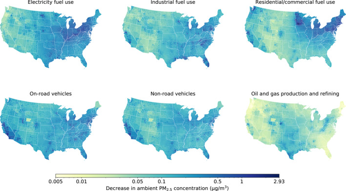
County‐level decrease in ambient PM_2.5 concentrations from the independent removal of PM_2.5, SO₂, and NO_x emissions in each of the six energy‐related sectors. Incongruous results for Sweetwater County, WY, in the on‐road vehicle, non‐road vehicle, and oil and gas production and refining sectors are likely the result of a model artifact.

We find a strong positive linear relationship between COBRA baseline PM_2.5 concentrations and AQS county‐average monitoring data from 2016 (r = 0.83, n = 604; Figure S3 in Supporting Information S1). For the 604 counties with AQS monitors, COBRA reported a slightly lower average baseline concentration (6.94 μg/m³) than the monitor average (7.27 μg/m³).

3.2. Total Attributable Mortality

We find that PM_2.5 exposure from all emissions sources led to 205,000 (95% CI: 180,000–230,000) premature deaths in the US in 2016. The mean value from this central estimate falls within the uncertainty range of results using COBRA's high estimate (247,000 [95% CI: 186,000–306,000]) and is well above results using COBRA's low estimate (112,000 [95% CI: 93,700–130,000]). Our central estimate is toward the higher end of the range of totals reported in previous studies. Figure 3 compares our mortality estimates to those from other recent studies using various air quality models, model years, and mortality functions. We discuss these results in more detail in Section 4 and more information is available in Table S3 in Supporting Information S1.

Figure 3.

Comparison of attributable mortality estimates from this and other studies using various air quality models and concentration‐response functions. Models and mortality functions used are detailed in Table S3 in Supporting Information S1.

3.3. Nationwide Health Benefits

We find that nationwide elimination of PM_2.5‐related emissions from energy‐related sources would prevent 53,200 (95% CI: 46,900–59,400) premature deaths and provide $608 billion ($537–$678 billion) in annual benefit from avoided PM_2.5‐related illness and death each year (Table 1). Other benefits include the prevention of 2,810–25,600 non‐fatal heart attacks, 15,000 asthma‐related emergency room visits, and 3.68 million days of work lost due to illness. Avoided premature mortality accounts for more than 98% of the total monetized benefits.

Table 1.

Health Benefits From Nationwide Elimination of Energy‐Related Emissions Sources

Health endpoint		Avoided impact
Premature adult mortality a	Central (age 25–99)	53,200 (46,900–59,400)
	High (age 25–99)	64,300 (48,100–80,500)
	Low (age 30–99)	28,600 (23,900–33,300)
Mortality and morbidity, total	Central	$608 billion ($537–$678 billion)
	High	$733 billion ($550–$914 billion)
	Low	$327 billion ($274–$380 billion)
Infant mortality, all‐cause (age <1)		175
Non‐fatal heart attacks (age 18–99)		2,810–25,600
Respiratory hospital admissions	Direct (age 65–99)	4,290
	Asthma (age 0–17)	575
	Chronic lung disease (age 18–64)	1,620
	Total	6,490
Cardiovascular hospital admissions, except heart attacks (age 18–99)		6,550
Acute bronchitis (age 8–12)		39,000
Upper respiratory symptoms (age 9–11)		727,000
Lower respiratory symptoms (age 7–14)		500,000
Asthma‐related emergency room visits (age 0–99)		15,000
Minor restricted‐activity days (age 18–64)		21.8 million
Work loss days (age 18–64)		3.68 million
Asthma exacerbation (age 6–18)		757,000

Note. Dollar values are for 2020. Values may not sum to total due to rounding. Ranges reflect 95% confidence intervals based on the beta coefficient of the standard error of the mean in the concentration‐response relationships.

^a The central estimate is calculated using the concentration‐response function from Burnett et al. (2018) and is for non‐accidental mortality; the low and high estimates, from Krewski et al. (2009) and Lepeule et al. (2012), respectively, are for all‐cause mortality.

The contribution of each sector to avoided mortality is shown in Table 2. Emissions removal in the on‐road vehicle sector prevents the most deaths (11,700), followed by residential/commercial fuel use (11,100) and electricity fuel use (9,260). Eliminating emissions from industrial fuel use prevents 8,990 premature deaths, the non‐road vehicle sector prevents 8,910 deaths, and oil and gas production and refining prevents 1,480 deaths. The summed avoided mortality count from independent emissions removal in the six sectors totals 51,400 premature deaths, which is 3.41% lower than from simultaneous emissions removal in all sectors. This slight discrepancy is due to differences in estimated PM_2.5 concentration changes in select counties between scenarios and the different method used to calculate avoided mortality from each sector independently versus simultaneously, as is discussed in Section 2.

Table 2.

Sector‐Level Breakdown of Avoided Premature Deaths and Total Monetized Health Benefits From Independent Emissions Removal

Sector	Avoided premature deaths			Monetized benefit (billion)
	Central	High	Low	Central	High	Low
Electricity fuel use	9,260	11,600	5,130	$106	$132	$59
Industrial fuel use	8,990	11,300	4,990	$103	$129	$57
Residential/commercial fuel use	11,100	13,900	6,160	$127	$159	$70
On‐road vehicles	11,700	14,700	6,490	$133	$168	$74
Non‐road vehicles	8,910	11,200	4,960	$102	$128	$57
Oil and gas production and refining	1,480	1,880	828	$17	$21	$9.5
Total	51,400	64,700	28,500	$588	$698	$327
All simultaneous	53,200	64,300	28,600	$608	$694	$327
Difference (%)	−3.41	0.55	−0.06	−3.35	0.55	−0.06

Note. Values may not sum to total due to rounding. Differences are the percent difference between the sum of sector‐level and total simultaneous emissions removal.

3.4. Regional and Interstate Flow of Health Benefits

We aggregate results from state‐level emissions removal scenarios by EPA region to determine the extent to which emissions removal in each region contributes to the accrual of health benefits in other regions. The states comprising each region are listed in Table S4 in Supporting Information S1, and a map of these regions is shown in Figure S4 in Supporting Information S1. Figure 4 shows the regional distribution of health benefits resulting from simultaneous emissions removal in all six sectors in each region. On average, slightly more than two‐thirds (69%) of the health benefits from emissions removal in a region—represented by our central estimate of avoided mortality—remain in the emitting region. Five of the 10 regions retain more than three‐quarters of the benefits from emissions removal in their region; just two retain less than half. The Southwest retains 95% of the health benefits from its own emissions removal while the Mountain region retains just 32% of the benefits from its own emissions removal. In fact, the Mountain region provides a greater combined portion of benefits to three other regions: the Midwest (14%), South Central (14%), and Southeast (12%).

Figure 4.

The distribution of health benefits by Environmental Protection Agency region. Values represent the portion of benefits, represented by the central mortality estimate, that accrue within a given region (columns) resulting from emissions removal from all six sectors in each region (rows). Darker colors indicate regions where higher portions of benefits accrue.

The range of portion of benefits remaining in an individual emitting state are even wider than when state results are summed by region. For example, just 3% of the benefits from emissions removal in Wyoming remain in Wyoming while 94% of benefits from emissions removal in California remain in California. On average, slightly less than half (45%) of the health benefits from emissions removal in a state remain in that state. A total of 8 states retain less than 25% of the benefits from in‐state emissions removal, 21 retain 25%–50%, 17 retain 50%–75%, and just 3 retain more than 75% of the benefits from their own emissions removal. States that retain a greater portion of benefits from their own emissions removal tend to have higher populations. The full breakdown of benefits by state is detailed in Table S5 in Supporting Information S1.

While the portion of health benefits that remain in an emitting region varies, the number of avoided deaths within an emitting region is substantial in all regions (Figure 5, dark blue bars). These values range from a low of 568 avoided premature deaths in the Mountain region to a high of 8,490 in the Midwest. All regions receive more benefit from nationwide action than independent regional action; the ratio of the light and dark blue bars in Figure 5 indicates the additional benefit a region would receive from nationwide efforts to eliminate emissions. The Southwest (1.07) and Northwest (1.13) see less than 25% more benefit from nationwide action. Four regions get between 25% and 50% more benefit from nationwide action: South Central (1.28), Midwest (1.31), Southeast (1.34), and Mountain (1.36). The Mid‐Atlantic (1.56), NY/NJ (1.76), and New England (1.87) see between 50% more and two times as much benefit. Only the Great Plains (2.17) gets more than two times as much benefit from nationwide action as from regional action. The full list of benefits by region is available in Table S6 in Supporting Information S1.

Figure 5.

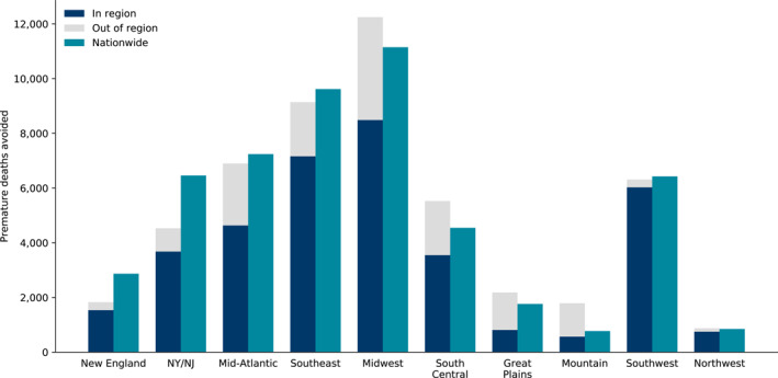
Avoided premature deaths resulting from emissions removal from all sectors in each region. Dark blue bars indicate the benefit a region would retain from independent emissions removal in that region, gray bars indicate the benefit that a region would pass on to all other regions from independent emissions removal in that region, and light blue bars indicate the benefit a region would receive from nationwide emissions removal.

As with results at the region level, all states see more benefit from nationwide action to eliminate emissions than state‐level action (average of 2.55 times as much), but the ratio of benefits varies more widely for states than for regions. California (1.07), for example, gets just 7% more benefit from nationwide action as it does from independent state‐level action while South Dakota (6.70) gets nearly seven times as much benefit from nationwide action. Three states get less than 25% more benefit from nationwide action as state‐level action. Five states get between 25% and 50% more benefit, eight states get between 50% more and two times as much benefit, and 19 see between two and three times as much benefit. Ten states get between three and four times as much benefit, and four states see more than four times as much benefit from nationwide action as state‐level action.

3.5. Comparison to Other Studies

We find strong agreement between our estimates of avoidable premature mortality and estimates of attributable mortality reported by Thakrar et al. (2020). As shown in Figure 6, our adjusted mortality estimate of 47,200 differs by just 4% and 2%, respectively, from the totals using InMAP (49,300) and EASIUR (46,400) reported by Thakrar et al. (2020). Our low mortality estimate (28,600) is 23% lower than the value reported by Thakrar et al. (2020) using AP2 (37,100).

Figure 6.

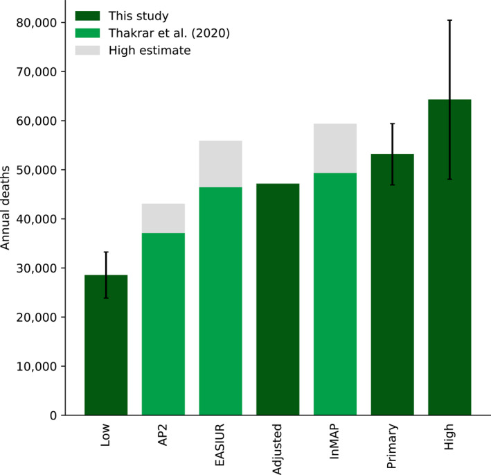
Comparison of mortality estimates for all six energy‐related sector using CO‐Benefits Risk Assessment, AP2, Estimating Air pollution Social Impact Using Regression (EASIUR), and Intervention Model for Air Pollution (InMAP). Error bars reflect ranges as represented by 95% confidence intervals based on the beta coefficient of the standard error of the mean in the concentration‐response relationships.

4. Discussion

We find that eliminating energy‐related sources of PM_2.5 pollution in the US would provide substantial health benefits from improved air quality. Removing emissions of primary PM_2.5, SO₂, and NO_x from the electric power, transportation, building, and industrial sectors nationwide in the US could prevent 53,200 (95% CI: 46,900–59,400) premature deaths and yield $608 billion ($537–$678 billion) in air quality‐related health benefits each year. We also explore the regional distribution of health benefits from regional and nationwide action to eliminate emissions. Between 32% and 95% of the health benefits from emissions removal that occur in a region remain in that region. All regions receive more benefit from nationwide emissions removal than they do from regional action, but the amounts range from just 1.07 times as much in the Southwest to 2.17 times as much in the Great Plains. These patterns are even more pronounced at the state level. States see an average of 2.55 times as much benefit (range: 1.07–6.70) from nationwide action as state‐level action. These findings indicate that some regions and states would be best served by concerted nationwide actions to reduce emissions given how much benefit is the result of emissions reductions in other places. Some regions and states, however, can get nearly as much benefit from removing emissions sources within their jurisdiction as they do from nationwide efforts. In any case, all regions can prevent hundreds or thousands of deaths by eliminating energy‐related emissions sources within the region, which shows the local benefits of local action to mitigate air quality issues.

Our estimates of total attributable mortality from PM_2.5 exposure from all emissions sources in the US falls within the range of estimates reported in previous studies. Estimates reported in the literature vary widely, in large part because of the choice of mortality function. Burnett et al. (2018) estimated 213,000 deaths from PM_2.5 exposure in 2015, within our reported range of 205,000 (95% CI: 180,000–230,000), using the same mortality function. (Note: the Burnett et al. (2018) total is for the US and Canada.) Using the mortality function described by Nasari et al. (2016) and parameterized by Tessum et al. (2019), we estimate 143,000 deaths from PM_2.5, Tessum et al. (2019) estimated 131,000 deaths, and Thakrar et al. (2020) estimated 99,900 deaths (InMAP) and 107,000 deaths (EASIUR), though estimates from Thakrar et al. (2020) are for human‐caused emissions, not all emissions sources as in this study.

We find that our estimates of avoidable mortality from the removal of energy‐related emissions sources agree closely with studies of source‐specific mortality that employ other RCMs used extensively in the literature (Figure 5). Using the same mortality function, our estimate of nationwide avoidable PM_2.5 deaths is within 2% and 4% of those reported by Thakrar et al. (2020) using EASIUR and InMAP. These results bolster the case for using COBRA in health impact assessments, particularly when reporting health effects at the national or regional level. However, other models such as InMAP can provide information about pollutant concentrations and associated health effects at finer spatial scales in populated areas than COBRA can given that COBRA reports results at the county level (Tessum et al., 2017). In nearly every sector we analyze, emissions of PM_2.5, SO₂, and NO_x have declined in the years since the emissions inventory used in this analysis was developed, so it is likely that some portion of the potential benefits we describe have already been realized (U.S. EPA, 2021a).

Our results on the regional flow of health benefits of energy‐related emissions removal reveal important similarities and differences with other work. Sergi et al. (2020) found that for all EPA regions, the majority of deaths from PM_2.5 exposure from all emissions sources in 2014 were the result of emissions within the same region. Compared to damages remaining in an emitting region reported by Sergi et al. (2020), we find that New England and NY/NJ retain higher portions of benefits from the removal of their energy‐related emissions sources; the Great Plains, Midwest, Mountain, and South Central regions retain lower portions; and the Mid‐Atlantic, Northwest, Southeast, and Southwest retain similar portions. Table S7 in Supporting Information S1 provides a comparison by region. While we cannot fully determine the reasons for these differences, it is likely that since Sergi et al. (2020) estimate death from all emissions sources and we calculate totals for energy‐related sources, their results are influenced more by emissions from ground‐level area sources not included in our analysis. Emissions from these types of sources tend to travel shorter distances and thus have greater health effects nearby the emission source than elevated point sources such as EGUs, which represent a greater share of emissions in our study. Penn et al. (2017), for example, found that an average of 22% of premature deaths from EGUs occurred in the emitting state, compared to 38% on average for residential fuel combustion, a ground‐level area source. They attribute this difference to the fact that most deaths from residential combustion are due to primary PM_2.5, whereas secondary PM_2.5 formed from SO₂ plays a larger role for EGUs. Dedoussi et al. (2020) find similar trends showing that SO₂ and NO_x caused a greater portion of deaths outside the emitting state than primary PM_2.5.

4.1. Limitations and Advantages

The S‐R matrix used in COBRA makes simplifying assumptions about the transport and chemical conversion of PM_2.5 components. These limitations are evidenced by the nearly identical PM_2.5 concentration changes from simultaneous emissions removal from all sectors and the sum of independent emissions removal from each of the six sectors in almost all counties. Past studies can help to illustrate the potential magnitude and direction of bias of our results stemming from this limitation. Dedoussi and Barrett (2014), for example, found notable differences in estimates of sector‐specific PM_2.5 mortality in the US in 2005 when comparing results from the Community Multiscale Air Quality (CMAQ) Modeling System, a state‐of‐the‐science CTM, to those from the GEOS‐Chem adjoint. They found that the mortality estimate from combustion sources from GEOS‐Chem was 13.9% higher than that from CMAQ. The largest difference occurred in the road transportation sector, for which GEOS‐Chem was 42.2% higher. Differences in other sectors were more modest: GEOS‐Chem was slightly higher for industrial combustion (12.9%) and commercial and residential combustion (10.6%), slightly lower for rail transportation (−4.9%) and marine transportation (−13.3%), and nearly identical for electric power generation (0.2%). The authors attribute some of the difference in sector‐level results to the fact that SO₂‐to‐sulfate chemistry, which dominates electric power sector impacts, is relatively linear compared to NO_x‐ and NH₃‐to‐nitrate chemistry, which play a greater role in transportation sectors. In another study, Dedoussi et al. (2020) found that modeling changes in emissions in primary PM_2.5, SO₂, NO_x, and NH₃ from all anthropogenic sources in the US simultaneously—to account for nonlinearities in interactions between emitted chemicals—produced a mortality estimate 30%–34% lower than when modeling each source independently. These studies suggest that our findings may slightly overestimate the health benefits of emissions removal, particularly in the on‐road vehicle sector, but that they likely differ by less than a factor of two.

Other studies report modest losses in fidelity when comparing RCMs to CTMs. Gilmore et al. (2019) determined that the marginal social cost of one ton of PM_2.5 emissions and its precursors reported by AP2, EASIUR, and InMAP were similar to those from the Weather Research and Forecasting model coupled with Chemistry (WRF‐Chem). The authors find that differences in marginal changes are not large or cancel out among different pollutants and locations, which is part of why we restrict our analysis to the national, regional, and state levels even though COBRA reports county‐level results. Tessum et al. (2017) found that COBRA performed similarly to InMAP in reproducing WRF‐Chem estimates of PM_2.5 concentration changes for 11 emissions scenarios in which total PM_2.5 concentrations changed by about 1%. These studies, however, examined much smaller emissions perturbations and resulting changes in PM_2.5 concentrations than those reported in our study. Buonocore et al. (2021) reported trends in agreement between RCMs over time and found that AP2, EASIUR, and InMAP produced more similar mortality estimates in 2008 than in 2017 for seven of eight emissions sources studied. The authors attribute this divergence in model results over time to changing emissions profiles. Coal combustion for electricity generation, for which the three models had good agreement, was the largest contributor to health impacts in 2008, mostly from SO₂ emissions. By 2017, however, emissions from coal had decreased and other sources, fuels, and pollutant types contributed greater shares of health impacts. This and other studies have found that models tend to have better agreement for SO₂ than for other PM_2.5 components (Buonocore et al., 2019; Gilmore et al., 2019).

While the choice of air quality model and limitations inherent within a given model can lead to important differences in modeled ambient PM_2.5 changes and resulting health effects, methodological choices related to health impact modeling can also produce large differences in health effects estimates resulting from changes in air quality. Foremost among these methodological inputs is the choice of mortality function. The choice and shape of the mortality function used in health impact assessments has considerable bearing on results. Nasari et al. (2016) conducted an illustrative analysis in which linear and non‐linear mortality functions were used to estimate the number of deaths attributable to changes in ambient PM_2.5 concentrations in the US and Canada between 2000 and 2010. The mortality functions draw on evidence from two large cohort studies: the ACS Cancer Prevention Study II and the Canadian Census Health and Environment Cohort (Crouse et al., 2015; Pope et al., 2015). The combined effect of the choice and shape of the mortality function resulted in differences in mortality estimates as large as 39% in Canada and 67% in the US, assuming identical changes in PM_2.5 concentrations in all scenarios for each country. The population‐weighted PM_2.5 concentration change in the US was 3.7 μg/m³, nearly two times the 1.90 μg/m³ decrease we estimate from the removal of emissions from all six sectors in this study. Dedoussi and Barrett (2014) note that the differences in mortality estimates resulting from their choice to use CMAQ or the GEOS‐Chem adjoint, which we describe above, were within the uncertainty range of the CRF used. The low and high all‐cause mortality functions used in this study, in fact, produce mortality estimates that differ by more than a factor of two. Our central mortality estimate, likewise, is 86% higher than the low estimate, which is based on the CRF derived from Krewski et al. (2009) and is used extensively in the health‐air quality literature.

Other health impact modeling assumptions that bear on results include the effects of population growth and changing baseline mortality rates. In a study of the health benefits associated with reductions in on‐road emissions in the US from 2008 to 2017, Choma et al. (2021) found that applying 2017 population characteristics to a 2008 emissions scenario increased non‐accidental mortality totals by 13% compared to using 2008 population characteristics. Slightly more than half of this increase (6.9%) was due to population growth and the remainder was the result of higher mortality rates, which is due to population aging. Other work has characterized the net change in PM_2.5 mortality attributable to population growth, population aging, mortality rates, and exposure change in the US and elsewhere (Cohen et al., 2017). Our analysis does not account for changing population characteristics since it models the effects of instantaneous emissions removal. However, since emissions changes on the scale of those modeled here are likely to occur over decades, population characteristics will affect observed outcomes. The population and mortality datasets we use for our GEMM estimates (i.e., 2016 population counts and 2015 non‐accidental mortality rates) project growth in all age groups by 2050 and decreases in baseline mortality rates for all age groups. Incorporating the effect of population growth would increase our avoidable mortality estimates while including mortality rate changes would decrease our estimates; these factors would together result in a net increase in avoidable mortality estimates.

The sensitivity of study findings to health impact modeling choices should be considered as important as the choice of air quality model, particularly for analyses primarily concerned with estimating health effects of air quality improvements. We use the GEMM function described by Burnett et al. (2018) as our central estimate for several reasons. First, the GEMM function includes direct evidence of the relationship between PM_2.5 exposure and mortality down to concentrations as low as 2.4 μg/m³ and suggests that the per‐unit change in attributable mortality at low levels is much greater than is assumed by other functions. Second, GEMM provides estimates of mortality risk over nearly the entire global PM_2.5 exposure range, which makes our results more comparable to benefit assessments in other world regions using the same function. Finally, the functional form and uncertainty characterization method that GEMM uses is readily applied in health impact assessment tools.

The methods described here offer important advantages. They are not computationally intensive, use publicly available data and software, and are accessible to a wide range of users. Additionally, by modeling the effect of full removal of emissions sources, we do not need to determine where and by how much emissions would be reduced, which would be necessary for emissions reductions of less than 100% since emissions reductions vary regionally and do not scale linearly with fossil fuel capacity displacement (Millstein et al., 2017). Modeling instantaneous emissions removal allows us to isolate the effect of removal from other temporally varying confounders such as meteorology, patterns of baseline energy use, and the size, distribution, and underlying health of populations.

4.2. Implications for Policy and Future Research

Across the US, regions vary in terms of the proportion of health benefits that accrue in an emitting region, versus the proportion of benefits accruing to other regions. Localized health benefits may support state‐level decision‐making to advance climate and clean energy policy, while distributed health benefits highlight the potential for federal action to maximize health benefits of clean energy. However, even regions that retain as little as one‐third of benefits within the region can prevent close to 600 premature deaths each year. There are also regions and states for which coordinated nationwide efforts would yield much greater health benefits than could be realized by acting independently; 33 states get at least two times as much benefit from nationwide action as state‐level efforts. Our findings highlight the importance of promoting emissions reduction initiatives at all spatial scales and the role of regional cooperation in maximizing public health benefits, particularly for efforts that could bring dual benefits for climate change mitigation.

Our work shows that multi‐pollutant control efforts, including CO₂‐reduction initiatives, could bring substantial PM_2.5‐related health benefits. These benefits could be realized through state‐level policies, wider regional agreement, and/or national‐scale initiatives. There is evidence that messages about the near‐term public health benefits of climate and clean energy policy can increase support for it among the public (Maibach et al., 2010; Petrovic et al., 2014; Stokes & Warshaw, 2017), and clean air is often touted by advocates as a benefit of clean energy policies. Our results characterize the spatial relationships between energy system change and air‐quality health benefits. By quantifying how an individual state or regional benefits from their own emissions reductions, compared to nationwide actions, energy and environmental policies can be designed in ways that engage stakeholders and advance public health across spatial scales.

While our analysis does not disaggregate health effects by race, ethnicity, or income, disparities in air pollution exposure across lines of race and class are well documented (Bell & Ebisu, 2012; Jbaily et al., 2022; Kravitz‐Wirtz et al., 2016; Tessum et al., 2019, 2021; Woo et al., 2019). Tessum et al. (2021), for example, found that people of color in the US are exposed to higher‐than‐average PM_2.5 levels from most emissions sources. These disparities were evident across income and exposure levels as well as within individual states, urban areas, and rural areas. Other work has found that higher levels of racial segregation in residential housing is associated with higher levels of air pollution exposure for many racial and ethnic minority groups (Woo et al., 2019). Understanding and addressing the underlying sociopolitical and economic factors that contribute to these differences are important for advancing environmental justice.

Our analysis highlights important directions for future research. The transition to a clean energy economy will take place over decades. Combining health impact modeling with sector‐specific energy system modeling would allow for a clearer understanding of the relative timing and scale of health benefits by sector and provide insight into the cumulative benefits accrued over the lifetime of decarbonization efforts.

Overall, our study reinforces and expands on findings from previous studies showing the substantial health benefits associated with energy‐related emissions reductions, evaluates the regional and state flow of benefits, and provides a suggestion of the scale of air quality‐related health benefits that could accompany deep decarbonization efforts. These results offer a clear rationale for mitigating climate change on public health grounds, showing that the sooner the US acts to reduce emissions, the more preventable death and disease from energy‐related air pollution can be avoided.

Conflict of Interest

The authors declare no conflicts of interest relevant to this study.

Supporting information

Supporting Information S1

Mailloux, N. A. , Abel, D. W. , Holloway, T. , & Patz, J. A. (2022). Nationwide and regional PM_2.5‐related air quality health benefits from the removal of energy‐related emissions in the United States. GeoHealth, 6, e2022GH000603. 10.1029/2022GH000603

Data Availability Statement

CO‐Benefits Risk Assessment is available for download at https://www.epa.gov/cobra. EPA AQS PM_2.5 monitor data are available at https://aqs.epa.gov/aqsweb/airdata/download_files.html. Environmental Benefits Mapping and Analysis Program Community Edition, from which population and mortality incidence data were extracted, is available for download at https://www.epa.gov/benmap.

References

- Barbose, G. , Wiser, R. , Heeter, J. , Mai, T. , Bird, L. , Bolinger, M. , et al. (2016). A retrospective analysis of benefits and impacts of U.S. renewable portfolio standards. Energy Policy, 96, 645–660. 10.1016/j.enpol.2016.06.035 [DOI] [Google Scholar]
- Bell, M. L. , & Ebisu, K. (2012). Environmental inequality in exposures to airborne particulate matter components in the United States. Environmental Health Perspectives, 120(12), 1699–1704. 10.1289/ehp.1205201 [DOI] [PMC free article] [PubMed] [Google Scholar]
- Buonocore, J. J. , Hughes, E. J. , Michanowicz, D. R. , Heo, J. , Allen, J. G. , & Williams, A. (2019). Climate and health benefits of increasing renewable energy deployment in the United States. Environmental Research Letters, 14(11), 114010. 10.1088/1748-9326/ab49bc [DOI] [Google Scholar]
- Buonocore, J. J. , Luckow, P. , Norris, G. , Spengler, J. D. , Biewald, B. , Fisher, J. , & Levy, J. I. (2016). Health and climate benefits of different energy‐efficiency and renewable energy choices. Nature Climate Change, 6(1), 100–105. 10.1038/nclimate2771 [DOI] [Google Scholar]
- Buonocore, J. J. , Salimifard, P. , Michanowicz, D. R. , & Allen, J. G. (2021). A decade of the U.S. energy mix transitioning away from coal: Historical reconstruction of the reductions in public health burden of energy. Environmental Research Letters, 16, 054030. 10.1088/1748-9326/abe74c [DOI] [Google Scholar]
- Bureau of Transportation Statistics . (2021). National Transportation Statistics 2021, 50th anniversary edition. U.S. Department of Transportation. Retrieved from https://www.bts.gov/topics/national-transportation-statistics [Google Scholar]
- Burnett, R. , Chen, H. , Szyszkowicz, M. , Fann, N. , Hubbell, B. , Pope, C. A. , et al. (2018). Global estimates of mortality associated with long‐term exposure to outdoor fine particulate matter. Proceedings of the National Academy of Sciences, 115(38), 9592–9597. 10.1073/pnas.1803222115 [DOI] [PMC free article] [PubMed] [Google Scholar]
- California Executive Order N‐79‐20 . (2020). Retrieved from https://www.gov.ca.gov/wp-content/uploads/2020/09/9.23.20-EO-N-79-20-Climate.pdf
- Choma, E. F. , Evans, J. S. , Gómez‐Ibáñez, J. A. , Di, Q. , Schwartz, J. D. , Hammitt, J. K. , & Spengler, J. D. (2021). Health benefits of decreases in on‐road transportation emissions in the United States from 2008 to 2017. Proceedings of the National Academy of Sciences, 118(51), e2107402118. 10.1073/pnas.2107402118 [DOI] [PMC free article] [PubMed] [Google Scholar]
- Cohen, A. J. , Brauer, M. , Burnett, R. , Anderson, H. R. , Frostad, J. , Estep, K. , et al. (2017). Estimates and 25‐year trends of the global burden of disease attributable to ambient air pollution: An analysis of data from the Global Burden of Disease Study 2015. The Lancet, 389, 1907–1918. 10.1016/s0140-6736(17)30505-6 [DOI] [PMC free article] [PubMed] [Google Scholar]
- Crouse, D. L. , Peters, P. A. , Hystad, P. , Brook, J. R. , van Donkelaar, A. , Martin, R. V. , et al. (2015). Ambient PM2.5, O3, and NO2 exposures and associations with mortality over 16 years of follow‐up in the Canadian Census Health and Environment Cohort (CanCHEC). Environmental Health Perspectives, 123(11), 1180–1186. 10.1289/ehp.1409276 [DOI] [PMC free article] [PubMed] [Google Scholar]
- Dedoussi, I. C. , & Barrett, S. R. H. (2014). Air pollution and early deaths in the United States. Part II: Attribution of PM2.5 exposure to emissions species, time, location and sector. Atmospheric Environment, 99, 610–617. 10.1016/j.atmosenv.2014.10.033 [DOI] [Google Scholar]
- Dedoussi, I. C. , Eastham, S. D. , Monier, E. , & Barrett, S. R. H. (2020). Premature mortality related to United States cross‐state air pollution. Nature, 578(7794), 261–265. 10.1038/s41586-020-1983-8 [DOI] [PubMed] [Google Scholar]
- Dimanchev, E. G. , Paltsev, S. , Yuan, M. , Rothenberg, D. , Tessum, C. W. , Marshall, J. D. , & Selin, N. E. (2019). Health co‐benefits of sub‐national renewable energy policy in the US. Environmental Research Letters, 14(8), 085012. 10.1088/1748-9326/ab31d9 [DOI] [Google Scholar]
- Fann, N. , Lamson, A. D. , Anenberg, S. C. , Wesson, K. , Risley, D. , & Hubbell, B. J. (2012). Estimating the national public health burden associated with exposure to ambient PM2.5 and ozone. Risk Analysis, 32(1), 81–95. 10.1111/j.1539-6924.2011.01630.x [DOI] [PubMed] [Google Scholar]
- Gallagher, C. L. , & Holloway, T. (2020). Integrating air quality and public health benefits in U.S. decarbonization strategies. Frontiers in Public Health, 8, 563358. 10.3389/fpubh.2020.563358 [DOI] [PMC free article] [PubMed] [Google Scholar]
- Gilmore, E. A. , Heo, J. , Muller, N. Z. , Tessum, C. W. , Hill, J. D. , Marshall, J. D. , & Adams, P. J. (2019). An inter‐comparison of the social costs of air quality from reduced‐complexity models. Environmental Research Letters, 14(7), 074016. 10.1088/1748-9326/ab1ab5 [DOI] [Google Scholar]
- Goodkind, A. L. , Tessum, C. W. , Coggins, J. S. , Hill, J. D. , & Marshall, J. D. (2019). Fine‐scale damage estimates of particulate matter air pollution reveal opportunities for location‐specific mitigation of emissions. Proceedings of the National Academy of Sciences, 116(18), 8775–8780. 10.1073/pnas.1816102116 [DOI] [PMC free article] [PubMed] [Google Scholar]
- Grab, D. A. , Paul, I. , & Fritz, K. (2019). Opportunities for valuing climate impacts in U.S. state electricity policy. Institute for Policy Integrity, New York University School of Law. Retrieved from https://policyintegrity.org/publications/detail/opportunities-for-valuing-climate-impacts-in-u.s.-state-electricity-policy [Google Scholar]
- Haines, A. , & Ebi, K. (2019). The imperative for climate action to protect health. New England Journal of Medicine, 380(3), 263–273. 10.1056/nejmra1807873 [DOI] [PubMed] [Google Scholar]
- Hystad, P. , Yusuf, S. , & Brauer, M. (2020). Air pollution health impacts: The knowns and unknowns for reliable global burden calculations. Cardiovascular Research, 116, 1794–1796. 10.1093/cvr/cvaa092 [DOI] [PMC free article] [PubMed] [Google Scholar]
- Industrial Economics, Inc . (2019). Evaluating reduced‐form tools for estimating air quality benefits. Retrieved from https://www.epa.gov/sites/default/files/2020-09/documents/iec_rft_report_9.15.19.pdf [Google Scholar]
- Institute for Health Metrics and Evaluation . (2022). GBD compare. Institute for Health Metrics, University of Washington. Retrieved from https://vizhub.healthdata.org/gbd-compare/ [Google Scholar]
- Intergovernmental Panel on Climate Change . (2018). Global warming of 1.5°C. An IPCC Special Report on the impacts of global warming of 1.5°C above pre‐industrial levels and related greenhouse gas emissions pathways, in the context of strengthening the global response to the threat of climate change, sustainable development, and efforts to eradicate poverty. Retrieved from https://www.ipcc.ch/sr15/download/ [Google Scholar]
- Jbaily, A. , Zhou, X. , Liu, J. , Lee, T.‐H. , Kamareddine, L. , Verguet, S. , & Dominici, F. (2022). Air pollution exposure disparities across US population and income groups. Nature, 601(7892), 228–233. 10.1038/s41586-021-04190-y [DOI] [PMC free article] [PubMed] [Google Scholar]
- Klimont, Z. , Kupiainen, K. , Heyes, C. , Purohit, P. , Cofala, J. , Rafaj, P. , et al. (2017). Global anthropogenic emissions of particulate matter including black carbon. Atmospheric Chemistry and Physics, 17(14), 8681–8723. 10.5194/acp-17-8681-2017 [DOI] [Google Scholar]
- Kodros, J. K. , Wiedinmyer, C. , Ford, B. , Cucinotta, R. , Gan, R. , Magzamen, S. , & Pierce, J. R. (2016). Global burden of mortalities due to chronic exposure to ambient PM2.5 from open combustion of domestic waste. Environmental Research Letters, 11(12), 124022. 10.1088/1748-9326/11/12/124022 [DOI] [Google Scholar]
- Kravitz‐Wirtz, N. , Crowder, K. , Hajat, A. , & Sass, V. (2016). The long‐term dynamics of racial/ethnic inequality in neighborhood air pollution exposure, 1990–2009. Du Bois Review: Social Science Research on Race, 13(2), 237–259. 10.1017/s1742058x16000205 [DOI] [PMC free article] [PubMed] [Google Scholar]
- Krewski, D. , Jerrett, M. , Burnett, R. T. , Ma, R. , Hughes, E. , Shi, Y. , et al. (2009). Extended follow‐up and spatial analysis of the American Cancer Society Study linking particulate air pollution and mortality (HEI Research Report 140). Health Effects Institute. [PubMed] [Google Scholar]
- Lelieveld, J. , Klingmüller, K. , Pozzer, A. , Burnett, R. T. , Haines, A. , & Ramanathan, V. (2019). Effects of fossil fuel and total anthropogenic emission removal on public health and climate. Proceedings of the National Academy of Sciences, 116(15), 7192–7197. 10.1073/pnas.1819989116 [DOI] [PMC free article] [PubMed] [Google Scholar]
- Lepeule, J. , Laden, F. , Dockery, D. , & Schwartz, J. (2012). Chronic exposure to fine particles and mortality: An extended follow‐up of the Harvard Six Cities Study from 1974 to 2009. Environmental Health Perspectives, 120(7), 965–970. 10.1289/ehp.1104660 [DOI] [PMC free article] [PubMed] [Google Scholar]
- Maibach, E. W. , Nisbet, M. , Baldwin, P. , Akerlof, K. , & Diao, G. (2010). Reframing climate change as a public health issue: An exploratory study of public reactions. BMC Public Health, 10, 299. 10.1186/1471-2458-10-299 [DOI] [PMC free article] [PubMed] [Google Scholar]
- McCubbin, D. , & Sovacool, B. K. (2013). Quantifying the health and environmental benefits of wind power to natural gas. Energy Policy, 53, 429–441. 10.1016/j.enpol.2012.11.004 [DOI] [Google Scholar]
- Millstein, D. , Wiser, R. , Bolinger, M. , & Barbose, G. (2017). The climate and air‐quality benefits of wind and solar power in the United States. Nature Energy, 2(9), 17134. 10.1038/nenergy.2017.134 [DOI] [Google Scholar]
- Nasari, M. M. , Szyszkowicz, M. , Chen, H. , Crouse, D. , Turner, M. C. , Jerrett, M. , et al. (2016). A class of non‐linear exposure‐response models suitable for health impact assessment applicable to large cohort studies of ambient air pollution. Air Quality, Atmosphere & Health, 9(8), 961–972. 10.1007/s11869-016-0398-z [DOI] [PMC free article] [PubMed] [Google Scholar]
- National Emissions Inventory Collaborative . (2019). 2016v1 Modeling Platform. Retrieved from http://views.cira.colostate.edu/wiki/wiki/10202 [Google Scholar]
- Patz, J. A. , Frumkin, H. , Holloway, T. , Vimont, D. J. , & Haines, A. (2014). Climate change: Challenges and opportunities for global health. Journal of the American Medical Association, 312(15), 1565. 10.1001/jama.2014.13186 [DOI] [PMC free article] [PubMed] [Google Scholar]
- Patz, J. A. , Stull, V. J. , & Limaye, V. S. (2020). A low‐carbon future could improve global health and achieve economic benefits. Journal of the American Medical Association, 323(13), 1247–1248. 10.1001/jama.2020.1313 [DOI] [PubMed] [Google Scholar]
- Paulos, B. , Hua, C. , Leon, W. , Elamin, W. M. , & Donalds, S. (2021). Guide to 100% clean energy states. Clean Energy States Alliance, United States Climate Alliance. Retrieved from https://www.cesa.org/projects/100-clean-energy-collaborative/guide/ [Google Scholar]
- Penn, S. L. , Arunachalam, S. , Woody, M. , Heiger‐Bernays, W. , Tripodis, Y. , & Levy, J. I. (2017). Estimating state‐specific contributions to PM2.5‐ and O3‐related health burden from residential combustion and electricity generating unit emissions in the United States. Environmental Health Perspectives, 125(3), 324–332. 10.1289/ehp550 [DOI] [PMC free article] [PubMed] [Google Scholar]
- Petrovic, N. , Madrigano, J. , & Zaval, L. (2014). Motivating mitigation: When health matters more than climate change. Climatic Change, 126, 245–254. 10.1007/s10584-014-1192-2 [DOI] [Google Scholar]
- Pope, C. A. , Turner, M. C. , Burnett, R. T. , Jerrett, M. , Gapstur, S. M. , Diver, W. R. , et al. (2015). Relationships between fine particulate air pollution, cardiometabolic disorders, and cardiovascular mortality. Circulation Research, 116(1), 108–115. 10.1161/circresaha.116.305060 [DOI] [PubMed] [Google Scholar]
- Sergi, B. , Azevedo, I. , Davis, S. J. , & Muller, N. Z. (2020). Regional and county flows of particulate matter damage in the US. Environmental Research Letters, 15(10), 104073. 10.1088/1748-9326/abb429 [DOI] [Google Scholar]
- Stokes, L. C. , & Warshaw, C. (2017). Renewable energy policy design and framing influence public support in the United States. Nature Energy, 2(8), 17107. 10.1038/nenergy.2017.107 [DOI] [Google Scholar]
- Tessum, C. W. , Apte, J. S. , Goodkind, A. L. , Muller, N. Z. , Mullins, K. A. , Paolella, D. A. , et al. (2019). Inequity in consumption of goods and services adds to racial–ethnic disparities in air pollution exposure. Proceedings of the National Academy of Sciences, 116(13), 6001–6006. 10.1073/pnas.1818859116 [DOI] [PMC free article] [PubMed] [Google Scholar]
- Tessum, C. W. , Hill, J. D. , & Marshall, J. D. (2017). InMAP: A model for air pollution interventions. PLoS One, 12(4), e0176131. 10.1371/journal.pone.0176131 [DOI] [PMC free article] [PubMed] [Google Scholar]
- Tessum, C. W. , Paolella, D. A. , Chambliss, S. E. , Apte, J. S. , Hill, J. D. , & Marshall, J. D. (2021). PM2.5 polluters disproportionately and systemically affect people of color in the United States. Science Advances, 7(18), eabf4491. 10.1126/sciadv.abf4491 [DOI] [PMC free article] [PubMed] [Google Scholar]
- Thakrar, S. K. , Balasubramanian, S. , Adams, P. J. , Azevedo, I. M. L. , Muller, N. Z. , Pandis, S. N. , et al. (2020). Reducing mortality from air pollution in the United States by targeting specific emission sources. Environmental Science and Technology Letters, 7(9), 639–645. 10.1021/acs.estlett.0c00424 [DOI] [Google Scholar]
- The White House . (2021). Fact sheet: President Biden sets 2030 greenhouse gas pollution reduction target aimed at creating good‐paying union jobs and securing U.S. leadership on clean energy technologies. Retrieved from https://www.whitehouse.gov/briefing-room/statements-releases/2021/04/22/fact-sheet-president-biden-sets-2030-greenhouse-gas-pollution-reduction-target-aimed-at-creating-good-paying-union-jobs-and-securing-u-s-leadership-on-clean-energy-technologies/ [Google Scholar]
- United Nations Environment Programme . (2020). The emissions gap report 2020. Retrieved from https://www.unep.org/emissions-gap-report-2020 [Google Scholar]
- U.S. CDC . (2022). CDC WONDER. Retrieved from https://wonder.cdc.gov/ [Google Scholar]
- U.S. EPA . (2021a). Air pollutant emissions trends data. Retrieved from https://www.epa.gov/air-emissions-inventories/air-pollutant-emissions-trends-data [Google Scholar]
- U.S. EPA . (2021b). CO‐Benefits Risk Assessment (COBRA) Health Impacts Screening and Mapping Tool. Retrieved from https://www.epa.gov/statelocalenergy/co-benefits-risk-assessment-cobra-health-impacts-screening-and-mapping-tool [Google Scholar]
- U.S. EPA . (2021c). Criteria air pollutants. Retrieved from https://www.epa.gov/criteria-air-pollutants [Google Scholar]
- U.S. EPA . (2021d). Environmental Benefits Mapping and Analysis Program–Community Edition (BenMAP–CE). Retrieved from https://www.epa.gov/benmap [Google Scholar]
- U.S. EPA . (2022a). Greenhouse gas inventory data explorer. Retrieved from https://cfpub.epa.gov/ghgdata/inventoryexplorer/ [Google Scholar]
- U.S. EPA . (2022b). Interstate air pollution transport. Retrieved from https://www.epa.gov/interstate-air-pollution-transport [Google Scholar]
- U.S. EPA . (2021e). Outdoor air quality data: Pre‐generated data files. Retrieved from https://aqs.epa.gov/aqsweb/airdata/download_files.html [Google Scholar]
- U.S. EPA . (2022c). Overview of the Cross‐State Air Pollution Rule (CSAPR). Retrieved from https://www.epa.gov/csapr/overview-cross-state-air-pollution-rule-csapr [Google Scholar]
- U.S. EPA . (2021f). Regional and geographic offices. Retrieved from https://www.epa.gov/aboutepa/regional-and-geographic-offices [Google Scholar]
- U.S. EPA . (2020). User’s manual for the CO‐Benefits Risk Assessment Health Impacts Screening and Mapping Tool (COBRA). Retrieved from https://www.epa.gov/cobra/users-manual-co-benefits-risk-assessment-cobra-screening-model [Google Scholar]
- U.S. EPA . (2021g). Visibility – Regional planning organizations. Retrieved from https://www.epa.gov/visibility/visibility-regional-planning-organizations [Google Scholar]
- Weagle, C. L. , Snider, G. , Li, C. , van Donkelaar, A. , Philip, S. , Bissonnette, P. , et al. (2018). Global sources of fine particulate matter: Interpretation of PM2.5 chemical composition observed by SPARTAN using a global chemical transport model. Environmental Science & Technology, 52(20), 11670–11681. 10.1021/acs.est.8b01658 [DOI] [PubMed] [Google Scholar]
- Wiser, R. , Millstein, D. , Mai, T. , Macknick, J. , Carpenter, A. , Cohen, S. , et al. (2016). The environmental and public health benefits of achieving high penetrations of solar energy in the United States. Energy, 113, 472–486. 10.1016/j.energy.2016.07.068 [DOI] [Google Scholar]
- Woo, B. , Kravitz‐Wirtz, N. , Sass, V. , Crowder, K. , Teixeira, S. , & Takeuchi, D. T. (2019). Residential segregation and racial/ethnic disparities in ambient air pollution. Race and Social Problems, 11(1), 60–67. 10.1007/s12552-018-9254-0 [DOI] [PMC free article] [PubMed] [Google Scholar]
- Woods & Poole Economics, Inc . (2015). 2012 complete US demographic database files. Retrieved from https://www.woodsandpoole.com/our-databases/united-states/all-geographies/ [Google Scholar]
References From the Supporting Information
- McDuffie, E. E. , Martin, R. V. , Spadaro, J. V. , Burnett, R. , Smith, S. J. , O’Rourke, P. , et al. (2021). Source sector and fuel contributions to ambient PM2.5 and attributable mortality across multiple spatial scales. Nature Communications, 12, 3594. 10.1038/s41467-021-23853-y [DOI] [PMC free article] [PubMed] [Google Scholar]
- Murray, C. J. L. , Avarkin, A. , Zheng, P. , Anvari, D. , Brauer, M. , Afshin, A. , et al. (2020). Global burden of 87 risk factors in 204 countries and territories, 1990–2019: A systematic analysis for the Global Burden of Disease Study 2019. The Lancet, 396(10258), 1223–1249. 10.1016/S0140-6736(20)30752-2 [DOI] [PMC free article] [PubMed] [Google Scholar]
- Shaddick, G. , Thomas, M. L. , Amini, H. , Broday, A. , Cohen, A. , Frostad, J. , & Green, A. (2018). Data integration for the assessment of population exposure to ambient air pollution for global burden of disease assessment. Environmental Science and Technology, 52(16), 9069–9078. 10.1021/acs.est.8b02864 [DOI] [PubMed] [Google Scholar]
- Vodonos, A. , Awad, Y. A. , & Schwartz, J. (2018). The concentration‐response between long‐term PM2.5 exposure and mortality: A meta‐regression approach. Environmental Research, 166, 677–689. 10.1016/j.envres.2018.06.021 [DOI] [PubMed] [Google Scholar]
- Vohra, K. , Vodonos, A. , Schwartz, J. , Marais, E. A. , Sulprizio, M. P. , & Mickley, L. J. (2021). Global mortality from outdoor fine particle pollution generated by fossil fuel combustion: Results from GEOS‐Chem. Environmental Research, 195, 110754. 10.1016/j.envres.2021.110754 [DOI] [PubMed] [Google Scholar]
Associated Data
This section collects any data citations, data availability statements, or supplementary materials included in this article.
Supplementary Materials