Design and Analysis Considerations for Utilizing a Mapping Function in a Small Sample, Sequential, Multiple Assignment, Randomized Trials with Continuous Outcomes^†

Abstract

Small sample, sequential, multiple assignment, randomized trials (snSMARTs) are multistage trials with the overall goal of determining the best treatment after a fixed amount of time. In snSMART trials, patients are first randomized to one of three treatments and a binary (e.g. response/non-response) outcome is measured at the end of the first stage. Responders to first stage treatment continue their treatment. Non-responders to first stage treatment are re-randomized to one of the other treatments. The same binary outcome is measured at the end of the first and second stages and data from both stages are pooled together to find the best first stage treatment. However, in many settings the primary endpoint may be continuous and dichotomizing this continuous variable may reduce statistical efficiency. In this manuscript, we extend the snSMART design and methods to allow for continuous outcomes. Instead of requiring a binary outcome at the first stage for re-randomization, the probability of staying on the same treatment or switching treatment is a function of the first stage outcome. Re-randomization based on a mapping function of a continuous outcome allows for snSMART designs without requiring a binary outcome. We perform simulation studies to compare the proposed design with continuous outcomes to standard snSMART designs with binary outcomes. The proposed design results in more efficient treatment effect estimates and similar outcomes for trial patients.

1 ∣. INTRODUCTION:

Recent developments have been made in small sample, sequential, multiple assignment, randomized trials (snSMARTs)^1,2 where the primary goal is identifying the best first stage treatment by sharing information across the two stages of the trial. In snSMARTs, patients are randomly assigned to a first treatment and a binary outcome (e.g. response) is measured at a fixed time point. The second stage treatment is assigned randomly or deterministically based on the design and response to first stage treatment. The same binary outcome is again measured at the end of the second stage. Data from the first and second stages are shared to determine the single best first stage treatment. This information-sharing design is beneficial in the setting of rare diseases. The attractiveness of using an snSMART design over a traditional single-stage design is that each patient contributes more information than in a single-stage design. snSMARTs may be preferable to traditional crossover designs in that patients who respond remain on treatment and those who do not respond switch to other treatments. While snSMARTs designs are similar to standard sequential, multiple assignment, randomized trials (SMARTs),³ they differ in their primary goal. Unlike SMARTs, the focus of an snSMART is not on estimating the effects of the embedded dynamic treatment regimens (DTRs) or tailored sequences of treatments, but rather in efficiently using two stages of information from the same individuals to find the best first stage treatment.

One ongoing snSMART is the A Randomized Multicenter Study for Isolated Skin Vasculitis (ARAMIS) trial.⁴ The goal of this trial is to determine the best treatment for isolated skin vasculitis, a rare disease. Currently, there are three treatments available for patients and all are prescribed routinely, and none are considered standard of care for this disease. As such, this trial has three active treatments as the three arms and there is no control arm. The snSMART design is appropriate since the number of patients is more of a limiting factor than the duration of the trial. Therefore, the longer duration of the trial due to the two stages was seen as a lower priority than needing to obtain as much information as possible from a limited number of patients.

One benefit of a multistage trial in rare disease settings is that there is more information obtained from an individual patient. The International Rare Diseases Research Consortium (IRDiRC) published a list of recommendations for rare disease clinical trial design in 2018.⁵ In these recommendations, they include using longitudinal data and using patients more than once. Multistage designs have been shown to have increased power relative to single stage designs.^1,6 This is due to having more information about the sources of variation.⁷ Single stage designs can only identify between treatment variation.⁷ Crossover designs and other multistage designs also can identify the between-patient variation⁷ resulting in less variation in the error term and more statistical efficiency. Even more powerful are snSMARTs where patients may stay on the same treatment so the variation between treatments and the variation between patients receiving the same treatment⁷ can both be identified.

Multistage designs such as a crossover design do not incorporate the patient outcome in the design. This is not ideal for rare diseases.^8,9 Second stage treatment assignment in snSMARTs and other multistage designs is often based on a binary outcome such that the trial protocol must specify a binary rule for what qualifies as a “response." Some procedures may dichotomize a continuous variable such as change in prostate specific antigen (PSA) in a prostate cancer trial¹⁰ or response may be determined using defined criteria such as Response Evaluation Criteria In Solid Tumors (RECIST). In an snSMART, the binary outcome must be the same at the end of the first and second stages and must be selected and agreed upon before the start of the trial.¹¹

However, in many studies the outcome of interest may not be a binary variable or there may not be enough information known about a continuous variable to dichotomize it for use in second stage randomization. Another recommendation from IRDiRC is to not dichotomize continuous endpoints.⁵ Dichotomizing a continuous outcome often results in lowered statistical efficiency.^12,13,14,5 In rare diseases, ensuring statistical efficiency is critical due to the inherently low number of patients in the trial.¹⁴ Further, results may vary based on the dichotomization strategy and cutoff selected.¹⁵

In rare diseases and rare cancers, selecting a robust, holistic outcome is ideal to capture the patient’s subjective experience and individual variations in the disease.^14,5,16 Patient reported outcomes (PROs) can be used to measure treatment benefit or risk¹⁷ and can record the full patient experience with a treatment. The primary endpoint of the ARAMIS trial is a dichotomized composite endpoint that incorporates PROs and clinical outcomes.⁴ The goal of the composite endpoint is to holistically capture both the disease clinical progression and the patient experience on the treatment. Dichotomized outcomes may miss critical information and may obfuscate results. A major drawback of implementing an snSMART in oncology and other chronic diseases is that efficacy and toxicity are both important outcomes and creating a dichotomous binary outcome that captures both outcomes effectively can be challenging.¹⁰ Dichotomizing a continuous outcome, such as a PRO or other composite endpoint, requires expansive knowledge on the outcome and treatment effects in order to select an appropriate dichotomization strategy.

Moreover, when the outcome of interest is a continuous variable, a clear choice for a dichotomization method or binary surrogate may not always be available prior to the start of a study. If a continuous variable is dichotomized, the cutoff selected will play a critical role in the trial progression. If the cutoff selected is too high and the majority of participants are categorized as non-responders, then most patients will switch treatments and the long term benefits of a treatment may not be observed. Conversely, if a cutoff is selected that is too low and the majority of participants are categorized as responders, then most patients will stay on the treatment and the effects of switching treatments will not be adequately observed and estimation errors in treatment effects may occur.

In small samples, this problem of identifying an appropriate cutoff is magnified as fewer patients in each treatment pathway will be observed with poorly selected cutoffs. Further, if a dichotomous response is used for the endpoint or outcome of a trial, as in a responder analysis, there is potential for significant loss in statistical power.^18,14 In small samples and rare disease settings, there may be few prior studies and less knowledge regarding the treatment effects on the outcome which further hinders the ability to select a suitable binary outcome. Additionally, the time and resources to run a pilot study to determine an appropriate cutoff are often not available in diseases and disorders that affect a small number of individuals.

Here we examine an snSMART design with a continuous outcome measured at the end of stages one and two where rerandomization depends on a mapping function of a continuous outcome as opposed to a binary outcome. This design leverages the additional information gained by a multistage design and better captures the effect of the treatment by using a continuous outcome. The ultimate aim is to estimate the expected first stage treatment effects for the multiple treatments being investigated in the snSMART. As in the ARAMIS trial, we assume that all treatments are used in practice and the goal is to identify the best first stage treatment. Examples of continuous outcomes with no clear dichotomization strategy are percent change, PROs, utility measures (or some combination of efficacy and toxicity), probabilities of response, or other composite endpoints. The trial design presented here allows for the implementation of an snSMART without requiring a binary first stage outcome to determine the next stage treatment for a patient. This method maintains the patient benefit of an snSMART by having an increased probability of switching treatments if an individual is not responding well on the current treatment and increased probability of staying on that treatment if the individual is responding well. It also maintains the benefit of being able to identify variation between treatments and between patients resulting in a more powerful design. In addition to allowing randomization to depend on a continuous outcome in the snSMART design, the methods presented here allow for continuous first and second stage outcomes as opposed to previous methods to analyze snSMART data that only applied to binary outcomes. Thus, due to continuous outcomes, we cannot use previously proposed methods for snSMARTs² and due to on second stage randomization depending on a continuous outcome and sharing information across stages for the first stage treatment effect, we cannot use standard SMART methods.

2 ∣. METHODS

2.1 ∣. snSMART design with a continuous mapping function

Here we present the proposed snSMART design which allows for a continuous outcome measured at the end of the first and second stages. This design does not require a binary outcome. In this design, all patients are randomized with equal probability to a first stage treatment. We measure the continuous outcome at the end of stage one for patient i, Y_i1, at a set time point, t. The probability of staying on the same treatment for patient i is a function of Y_i1, and we call this function, f(Y₁), the mapping function. The mapping function ranges between 0 to 1 in order to yield valid probabilities.This is similar to the idea of treatment effect mappings introduced by Rosenberger¹⁹, but only relies on the patient’s individual outcome and not the outcome of others. Patients randomized to switch treatments are randomized to one of the remaining treatments with equal probability. At a set final time point, 2t, the outcome at the end of stage two, Y_i2, is measured. A schematic of the traditional snSMART design is given in Figure 1A and the proposed snSMART design is presented in Figure 1B.

FIGURE 1.

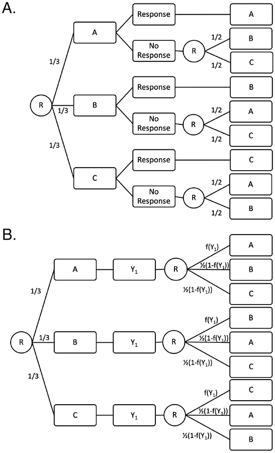
A traditional small sample, sequential, multiple assignment randomized trial (snSMART) design with a binary outcome (A) and the proposed snSMART design with a continuous outcome (B). A, B, and C are treatments, R indicates a randomization point, and f(Y₁) is the mapping function. Numbers indicate probability of assignment to the treatment following. Each stage is the same length so that Y₁ is measured at time t and Y₂ is measured at time 2t.

The randomization at the end of the first stage can be thought equivalently as a one-step randomization process or a two-step randomization process. The one step randomization proceeds as presented in Figure 1B where the next treatment is decided by a multinomial distribution with probabilities [f(Y₁), 0.5(1 − f(Y₁)), 0.5(1 − f(Y₁))] for staying on the same treatment and switching to either other treatment, respectively. It can also be thought of as a two-step randomization process with two binomial distributions (Web Figure 1). The first randomization determines if the patient stays or switches treatment and has probability of staying equal to f(Y₁). If the person switches treatments, then there is a second randomization with probability 0.5 for each remaining treatment.

2.1.1 ∣. The mapping function

The mapping function maps the first stage outcome, Y_i1, to [0, 1] and gives the probability of staying on the same treatment. More favorable values of the outcome map to values closer to 1 so that patients doing well on a treatment have a higher probability of staying on the same treatment. Depending on what is known about the outcome, various mapping functions can be selected. We provide examples of mapping functions and assume that higher values of Y indicate more favorable performance, but the functions are generalizable in other cases. While we offer the following suggestions, any cumulative distribution function can be used.

For areas of study with small samples such as rare diseases, there may be little information known about the distribution of Y₁. If only minimum and maximum values are known for Y₁, a linear mapping function f(Y₁) = (Y₁ − Y_min)/(Y_max − Y_min) can be used. This linear f(Y₁) function can be easily modified using powers for different trial characteristics. For example, if it is desirable for high proportions of patients stay on the same treatment through both stages, or if it is expected that the outcome may be right skewed, then using f(Y₁)^1/k, k > 1, may be appropriate. Likewise, if having more people switch is of interest or if the outcome is left skewed, then f(Y₁)^k, k > 1, may be appropriate.

If there are extreme values within this possible range of Y₁ that rarely occur, the linear function over the possible range of Y₁ may result in very few people on certain treatment regimens. For example, if Y₁ has a distribution as seen in Figure 2 (iii), then a linear mapping function will result in the majority of people switching treatments. To adjust for this, one can select a more practical minimum and maximum and then truncate the mapping function at 0 and 1. These values may represent safety and ethical limits in addition to the practicality of the study. The minimum could be the lowest value of Y₁ where investigators feel comfortable with a patient staying on the same treatment. This lower lower limit is a safety measure as it represents the worst outcome a patient will have and stay on the same treatment. The highest value of Y₁ is selected where investigators feel comfortable with a patient switching treatments, so that if a patient has a higher outcome they will stay on the current treatment. This upper limit represents an ethical boundary since it could be viewed as unethical to switch treatments for a patient responding this well to their current treatment. Patients can be consulted to aid in determining the upper and lower limits, which may make the trial more patient centered and appealing to patients.²⁰ Developing these extreme limits requires less prior knowledge regarding the treatment effects than is needed to effectively dichotomize a continuous outcome. Additionally, even when minimums and maximums are selected, the mapping function is more flexible than a binary outcome.

FIGURE 2.

Possible distributions of outcome Y and mapping functions that balance patients staying or switching treatments. The plots labelled distribution of Y are the probability distribution functions. The y-axis for plots labelled possible mapping functions is the probability of staying on the treatment for a given value of Y. Higher values of Y are assumed to indicate better outcomes.

2.2 ∣. Bayesian Analysis Methods

2.2.1 ∣. Model and likelihood

We assume the data from the snSMART design, has a multivariate normal likelihood:²¹

$$\left[\begin{array}{c}\hfill \hfill \\ \hfill Y_{i1}\hfill \\ \hfill \hfill \\ \hfill Y_{i2}\hfill \\ \hfill \hfill \end{array}\right]\mid T_{i1},T_{i2}\sim MVN(\left[\begin{array}{c}\hfill \hfill \\ \hfill {\mu }_1(T_{i1})\hfill \\ \hfill \hfill \\ \hfill {\mu }_2(T_{i1},T_{i2})\hfill \\ \hfill \hfill \end{array}\right],\mathbf{V}(T_{i1},T_{i,2}))$$

where Y_is is a continuous outcome and T_is is the treatment for patient i in stage s, s = 1, 2. The mean outcome for stage one, μ₁, is a function of only the first stage treatment. The mean for the second stage, μ₂, is a function of both the first and second stage treatments. The covariance matrix is a function of the sequence of treatments the patient received.

The mean treatment effects for stage one and two are modeled as follows for treatments A, B, and C:

$$\begin{gathered} {\mu }_1(T_{i1})=\sum _{j=A}^C{\beta }_{j}I(T_{i1}=j) \\ {\mu }_2(T_{i1},T_{i2})={\alpha }_1\sum _{j=A}^C{\beta }_{j}I(T_{i1}=j)+{\alpha }_2\sum _{k=A}^C{\beta }_{k}I(T_{i2}=k)+{\alpha }_{3}I(T_{i1}=T_{i2}) \end{gathered}$$ (1)

The β_j parameters are the expected effect of treatment j, j = A, B, C, in the first stage. The primary goal of an snSMART is to estimate these β_j parameters in order to identify the single best treatment during the first stage. The first stage mean outcome depends on the treatment effect for the treatment received in stage one. We model the second stage mean outcome as a weighted average of the treatment effects from stage one and stage two with an additional effect if the patient stays on the same treatment. Practically, this mean model for stage two can occur when there is some lingering effect of the first treatment (α₁) and some additional effect of the second treatment (α₂) when α₁, α₂ > 0. Alternatively, if the patient stays on the same treatment, the effect of the treatment in the second stage is the first stage effect with some cumulative effect that occurs on the treatment longer term (α₃). The proposed mean models allow for shared information between the two stages through β_j. The previously proposed linkage parameters in prior work to analyze data from an snSMART with binary outcomes² are similar to the α parameters that we use in our models.

For modeling the covariance, we use V(T_i1, T_i,2) = V₁I(T_i1 = T_i2) + V₂I(T_i1 ≠ T_i2) where V₁ and V₂ are both 2 × 2 variance-covariance matrices. This allows those who stay on the same treatment to have a different correlation between stage one and stage two outcomes than those who switch treatments.

Data from the snSMART design in Figure 1B can be analyzed using other mean models (e.g. to consider non-additive effects or effects of treatment specific pathways), but since our focus is on small samples, we present a parsimonious model where information sharing is feasible and the primary goal is to estimate and compare first stage treatments.

2.2.2 ∣. Prior distributions

We propose minimally informative prior distributions for all model parameters. For the treatment effects, βs, we use a normal prior with mean within the range of outcome Y. We suggest using the midpoint between Y_min and Y_max for the mean.

We impose three constraints regarding the α_m parameters, m = 1, 2, 3:

1. α₂ = 1 − α₁, α₁, α₂ > 0,

2. α₂ > α₁, and

3. α₃ ≥ 0.

Constraint 1 states that if a person does not stay on the same treatment then the second stage expected outcome is a weighted average of first stage outcomes the stage one and stage two treatments. This constraint facilitates estimation by requiring fewer variables to be estimated. Constraint 2 states that the second stage treatment has a larger effect on the second stage outcome than the first stage treatment. Constraint 3 states that staying on the same treatment has a non-negative effect on the expected second stage outcome. Constraints 2 and 3 reduce the parameter space and are therefore practical in many rare disease settings.

The prior for α₁ is set to be uniform from 0 to 0.5. Since we set α₂ = 1 - α₁ per constraint 1, this prior fulfills constraint 2 and forces α₂ > α₁ since α₁ will always be less than 0.5. Since we constrain α₃ to be non-negative, we use a folded normal (FN) distribution. For the prior on the covariance matrices, we use inverse Wishart (IW) distributions since they are the non-informative conjugate prior for multivariate normal covariances. Thus, suggested priors are as follows: β_j ~ N (mean = 50, standard deviation (sd) = 50) for all j, α₁ ~ Unif(0, 0.5), α₃ ~ FN(mean = 0, sd = 20), and V₁ and $V_2\sim I{W}_2\left(\left[\begin{array}{cc}\hfill 1\hfill & \hfill 0\hfill \\ \hfill 0\hfill & \hfill 1\hfill \end{array}\right],2\right)$.

2.2.3 ∣. Single-stage design

To examine the efficiency of the trial design of an snSMART with a mapping function, we compare it to a traditional singlestage design in which individuals are equally randomized to one of the three treatments. In the single-stage design, we analyze the outcome using the following Bayesian methods. Using the same notation as in section 2.2, we assume a normal likelihood:

$$Y_{i1}\mid T_{i1}\sim N\left({\mu }_1(T_{i1}),{\sigma }^2\right)$$

The mean μ₁(T_i1) is the same as in (1) and the βs have the same priors as in Section 2.2.2. The prior for σ is an inverse gamma, IG(1000, 1000).

3 ∣. SIMULATIONS

For each scenario, simulations were done with n = 100, 30, 15 in each treatment arm for total sample sizes of 300, 90, or 45. Results for n = 30 are presented here and results for n = 100 and 15 are presented in the supplemental material. Results are based on 2500 simulated trials. For analysis, we used the Bayesian analysis methods described in Section 2.2 with 1000 burn in and 5000 MCMC repetitions. We used R and rjags for simulations.

Our primary goal is accurate and efficient estimation of the effects of the treatments after the first stage in order to identify the best overall treatment. As such, we examine bias and root mean squared error (rMSE) of the estimates of β_j. Additionally, we examined patient outcomes and how many patients stayed on their current treatment or switched treatments.

3.1 ∣. Generation of Trial Data

Trial data was generated by first assigning n patients equally to each of three treatments. Stage one outcome was generated as Y₁ ~ N(μ₁(T₁), σ²) where σ² was the marginal variance for the first stage outcome. Based on this outcome, a patient was randomly assigned to a stay on the same treatment with probability f(Y₁) using Bernoulli(f(Y₁)) where f(·) was the mapping function. We set the parameters so that the range of Y was approximately 0-100. Correspondingly we set Y_min = 0 and Y_max = 100. We then investigated the three following mapping functions:

$$\begin{gathered} \text{MF}1=f_1(Y_1)=Y_1∕100 \\ \text{MF}1∕2=f_2(Y_1)=(Y_1∕100{)}^{1∕2} \\ \text{MF}2=f_3(Y_1)=(Y_1∕100{)}^2 \end{gathered}$$ (2)

For Y₁ outside the range of 0-100, these probabilities were truncated to be 0 or 1 respectively. Guidance for selecting the mapping function is provided in Section 2.1.1. If the patient did not stay on the same treatment, then the second treatment was randomly assigned using Bernoulli(0.5).

Let the ith row and jth column in V(T_i1, T_i,2) be denoted V_ij. Then the conditional means for the outcomes are:

$$\begin{gathered} Y_{i1}\mid T_{i1},T_{i2}\sim N({\mu }_1(T_{i1}),{\mathbf{V}}_{11}) \\ {Y}_{i2}\mid Y_{i1},T_{i1},T_{i2}\sim N\left({\mu }_2(T_{i1},T_{i2})+\frac{\sqrt{{\mathbf{V}}_{22}}}{\sqrt{{\mathbf{V}}_{11}}}{\mathbf{V}}_{12}(Y_{i1}-{\mu }_1(T_{i1})),(1-{\mathbf{V}}_{12}^2){\mathbf{V}}_{22}\right) \end{gathered}$$ (3)

The second outcome was generated from a conditional normal distribution in equation 3. For the single-stage design, only the first stage outcomes were used.

3.2 ∣. Scenarios

3.2.1 ∣. Ideal situations

As in Section 2.2.1, we let the covariance matrix be V(T_i1, T_i,2) = V₁I(T_i1 = T_i2) + V₂I(T_i1 ≠ T_i2) and we set V₁and V₂ to be:

$$V_1={\sigma }^2\left[\begin{array}{cc}\hfill 1\hfill & \hfill {\tau }_1\hfill \\ \hfill {\tau }_1\hfill & \hfill 1\hfill \end{array}\right],V_2={\sigma }^2\left[\begin{array}{cc}\hfill 1\hfill & \hfill {\tau }_2\hfill \\ \hfill {\tau }_2\hfill & \hfill 1\hfill \end{array}\right]$$

We set τ₁ = 0.8, τ₂ = 0.3, and σ = 20 (based on results from a validated ANCA-associated vasculitis PRO²²). For the mean model, we set α₁ = 0.2, α₃ = 0.8, α₃ = 5. We changed the β parameters to examine different effects of the mapping functions in scenarios such as presented in Figure 2. The β parameters are presented in Table 1 where scenarios 1, 2, and 3 are ideal scenarios where the model assumptions are met. These β values reflect possible values for a continuous outcome that has been standardized to range from 0-100 (e.g. this is typical in PRO development).^23,22

TABLE 1.

Simulation scenarios. Parameters are estimated as in equation 1 with any violations as described in Section 3.2.3. Treatment specific pathway (TSP) violates the mean model assumptions, Variance indicates that there are more variance parameters than are estimated, and Correlation indicates that there are more correlation parameters than estimated. β_j indicates the treatment effect of treatment j after a fixed amount of time and the study goal is to accurately and efficiently estimate these parameters.

	βj			Violation in Assumptions
Scenario	A	B	C	TSP	Variance	Correlation
1	40	50	60
2	20	30	40
3	60	70	80
4	40	50	60	×
5	40	50	60		×
6	40	50	60			×
7	40	50	60	×	×
8	40	50	60	×		×
9	40	50	60		×	×
10	40	50	60	×	×	×

3.2.2 ∣. Comparison with dichotomized outcome

This trial design that does not require a binary outcome (Figure 1B) will be primarily useful in cases when a binary outcome is not available. However, in simulations we are able to compare these the proposed design with a mapping function to an snSMART with a binary outcome (Figure 1A), even though in practice, a design with a well selected binary outcome may not be always feasible. We compare the three mapping functions in equation 2 with three binary outcomes based on dichotomizing the continuous outcome at the end of the first stage. If the patient’s outcome at the end of the first stage is above the cutoff, they stay on treatment, and if it is below the cutoff, they are equally randomized to one of the two remaining treatments. We investigated three cutoffs of 30, 50, and 70 for the binary outcome. We use scenarios 1, 2, and 3 (scenarios with no model assumption violations) in table 1 with these cutoffs to examine trial properties and compare with the mapping functions in equation 2. We compare the average patient outcomes and the number of patients on each sequence of treatments between the trial designs.

3.2.3 ∣. Model assumption violations

We examined three potential assumption violations individually and in combination as defined in Table 1, scenarios 4-10. In each scenario, the parts of the data generative model without assumption violations are the same as in scenario 1. First, we assumed the second stage mean was fully dependent on the combination and ordering of treatments the patients received in stages one and two (T_i1, T_i2) (i.e. not a weighted mean). We call this the treatment specific pathway (TSP) (column “TSP" in Table 1; scenarios 4, 7, 8, 10) and is essentially where there is an interaction between treatments. We set μ₂ = Σ_jΣ_k T_jkI(T_i1 = j, T_i2 = k) where

$$\mathbf{T}=\left[\begin{array}{ccc}\hfill 55\hfill & \hfill 43\hfill & \hfill 47\hfill \\ \hfill 40\hfill & \hfill 50\hfill & \hfill 60\hfill \\ \hfill 70\hfill & \hfill 65\hfill & \hfill 60\hfill \end{array}\right]$$

and T_jk indicates the jth row and kth column of matrix T_jk.

The second assumption violation was that we set the standard deviation of the outcome, σ, to depend on treatment (column “Variance" in Table 1; scenarios 5, 7, 9, 10). Here we set the standard deviation to be 10, 20, and 30 for treatments A, B, and C respectively.

The third assumption violation allowed the correlation between the first and second stage outcome to depend on the TSP (column “Correlation" in Table 1; scenarios 6, 8-10). Practically, this would arise if treatment outcomes have different correlation due to similarities in treatment mechanism even if the actual treatments differ. We set the correlations τ = Σ_j Σ_k R_jkI(T_i1 = j, T_i2 = k) where

$$\mathbf{R}=\left[\begin{array}{ccc}\hfill 0.85\hfill & \hfill 0.6\hfill & \hfill 0.2\hfill \\ \hfill 0.6\hfill & \hfill 0.8\hfill & \hfill 0.5\hfill \\ \hfill 0.2\hfill & \hfill 0.2\hfill & \hfill 0.9\hfill \end{array}\right]$$

and R_jk indicates the jth row and kth column of matrix R_jk.

To assess sensitivity to normally distributed outcomes, we also examined scenarios where the first stage outcome was a scaled Beta distribution rather than a normal distribution. The second stage was still conditionally normal but no longer marginally normal. We set the parameters of the Beta distribution such that the scaled means were the same as those in Scenarios 1, 2, and 3. We set the variance to be 0.1 prior to scaling.

4. ∣. RESULTS

R software code used for the simulations is available upon request.

4.1 ∣. Estimation of the treatment effect

4.1.1 ∣. Two-stage versus single-stage design

We first compare this two-stage snSMART design to a single-stage design with the same total number of patients but only one stage of treatment (and thus one outcome per patient). As expected, in scenarios 1, 2, and 3 we found large reductions in rMSE when comparing the two-stage design with the single-stage design regardless of the mapping function used (Table 2). The percent of trials that correctly identified the best treatment (determined by having the highest estimated first stage treatment effect) was consistently higher in the two-stage designs than the single-stage designs (Table 2), although all simulations resulted in >95% of trials identifying the true best treatment.

TABLE 2.

The root mean squared error (rMSE) for each β_j, j = A, B, C when estimated in a single-stage design and the proposed two-stage snSMART design. β_j indicates the treatment effect. Ratio is the rMSE divided by the rMSE of the single-stage design for that scenario. MF = mapping function, DO = dichotomized outcome (Section 3.1).

		rMSE			Ratio
Scenario	Design	βA	βB	βC	βA	βB	βC	Percent Correct
1	Single-Stage	3.65	3.69	3.51	1.00	1.00	1.00	97.40
	MF 1	2.97	3.01	2.87	0.82	0.82	0.80	99.52
	MF 1/2	3.02	2.93	2.84	0.83	0.79	0.81	99.40
	MF 2	3.00	3.09	3.15	0.82	0.84	0.90	99.24
	DO 50	5.57	5.58	5.15	1.53	1.51	1.47	99.16
	DO 30	5.32	3.92	3.19	1.46	1.06	0.91	99.35
	DO 70	2.87	3.52	4.80	0.79	0.95	1.37	99.15
2	Single-Stage	3.51	3.66	3.66	1.00	1.00	1.00	96.64
	MF 1	3.08	2.96	2.91	0.88	0.81	0.79	99.68
	MF 1/2	3.22	2.99	2.91	0.92	0.82	0.79	99.52
	MF 2	2.94	2.87	2.97	0.84	0.78	0.81	99.44
	DO 50	2.95	3.51	4.79	0.84	0.96	1.31	99.68
	DO 30	5.75	5.50	5.03	1.64	1.51	1.37	99.32
	DO 70	2.98	3.11	3.31	0.85	0.85	0.91	99.64
3	Single-Stage	3.64	3.66	3.67	1.00	1.00	1.00	97.36
	MF 1	3.04	3.00	2.92	0.83	0.82	0.79	99.28
	MF 1/2	3.02	2.90	2.87	0.83	0.79	0.78	99.60
	MF 2	3.19	3.22	3.19	0.88	0.88	0.87	99.08
	DO 50	5.20	3.81	3.15	1.43	1.04	0.86	98.67
	DO 30	2.99	2.96	2.89	0.82	0.81	0.79	99.40
	DO 70	5.65	5.74	5.23	1.55	1.57	1.43	96.87

4.1.2 ∣. Mapping function versus dichotomized outcome

In ideal scenarios (1-3), where the data generation model matched the analysis model, our method estimated the first stage treatment effects, β_j with minimal bias (Figure 3A). Bias and efficiency did not change substantially by changing the mapping function in scenarios 1, 2, and 3. Since the main goal of this trial design is to identify the best treatment from estimating the β_j parameters, low bias and high efficiency are both desirable trial traits.

FIGURE 3.

A. Box plots of bias averaged across the three β_j, j = A, B, C parameters for ideal scenarios where β_j indicates the treatment effect. A single point represent the average bias for one simulated trial. Light gray boxes are mapping functions (MF, Section 3.1) and dark gray boxes are dichotomized outcomes (DO, Section 3.2.2). B. Box plots of bias for each of the three β_j parameters in scenarios where assumptions are violated using MF 1. A single point represent the bias for one β_j in one simulated trial. Top labels indicate which scenario is being presented. Shades indicate the different β_j parameters.

Efficiency was similar between the mapping functions for each scenario (data not shown). Correspondingly, the coverage probability of the credible interval was close to the desired 95% and the credible interval width was consistent (Web Table 1). The coverage probability was lower for the small sample size of 15 patients per treatment arm (Web Table 2). Overall, the selection of the mapping function does not appear to have a substantial impact on the operating characteristics of the trial design when assumptions are met.

The results from using a dichotomized outcome vary considerably (Figure 3A). When the median treatment effect was selected as the cutoff, the bias was lowest, but the efficiency was worst as seen by the high variance (Figure 3A). Moderate bias was observed for other cutoffs due to poor estimates of the correlation parameters and α_m,m = 1 and 3. The quality of these estimates is dependent on the number of subjects that stay or switch and having a balance of people staying on the same treatment and switching treatments allows for better estimation of these parameters. The increased variance for the median cutoff is also related to the correlation and α_m, m = 1 and 3 parameter estimates. When these parameters and the correlation are fixed and do not need to be estimated, the bias is negligible and the variance in the bias estimates are consistent (Web Figure 2).

In general, the statistical performance was worse when using a binary outcome based on dichotomizing the outcome at the end of stage one than when using a continuous outcome with a mapping function. For some scenarios, binary outcomes performed similar to the mapping functions (Scenario 2, dichotomous outcome (DO) 70; Scenario 3, DO 30). However, the selection of the dichotomized outcome cutoff influences the model parameter estimation which is not ideal since the optimal cutoff value is not generally known in advance. For all scenarios, there were binary outcomes that performed worse than all mapping functions in terms of bias and efficiency. This indicates that poorly selected binary outcomes perform worse than any recommended mapping function. We additionally looked at mapping functions with a smaller range (25 to 75 instead of 0 to 100) and found that these functions also had improved performance over the dichotomized outcomes (Web Table 11).

The percent of trials that correctly identified the best treatment were similar between mapping functions and dichotomous outcomes where the mapping function performed slightly better (Table 2, Web Table 3). In a null scenario where all treatments have treatment effect of 50, each treatment was identified as the best approximately 33% of the time which is as expected (Web Table 9).

One difference between snSMARTs with a mapping function and snSMARTs with a binary outcome was the proportion of subjects that stayed on the same treatment (Web Table 6). The proportion that stayed on the same treatment had less variation under a mapping function than that from a binary outcome. In scenarios where the dichotomization strategy was a poor fit for the patient outcomes (i.e. the cutoff is either too high or too low), extreme results occurred where 3.2% stayed on treatment (scenario 2, DO 70) or where 96.8% switched treatments (scenario 3, DO 30). These same scenarios had somewhat less extreme results under a mapping function where 13.5% and 85% stayed on treatment respectively (scenario 2, mapping function (MF) 2; scenario 3, MF 1/2). Since some model parameters may be impossible to estimate if a trial concludes with no patients on a certain treatment path (i.e. if all patients stay on the same treatment or all switch treatments) having a moderate proportion of individuals that stay on the same treatment is preferable to avoid such extreme circumstances. Additionally, patients all stay or switch is beneficial to the patients if all are doing very well or very poorly respectively. However, having all patients stay may prevent some patients from trying other treatments that perform better and having all switch may mean that the patients do not experience the long term benefits of staying on a treatment.

4.1.3 ∣. Model Assumption Violations

Here we examine the effects on the results when model assumptions are violated. Unlike the ideal scenarios, the bias heavily depended on the β parameter being estimated (Web Table 4, Figure 3B). We examine when the second stage treatment effect is based on the treatment specific pathway (TSP) of the first and second stage treatments rather than a weighted average (scenarios 4, 7, 8, 10), variance is based on treatment and stage (scenarios 5, 7, 9, 10), and correlation is based on the two treatments received (scenarios 6, 8, 9, 10).

In general, the mean model violation caused the largest increase in bias (Figure 3B). Correlation and variance assumption violations did not result in increased bias suggesting that the estimates are some what robust to correlation and variance mis-specification. Similarly, the coverage probability for scenarios with the mean model assumption violation was more frequently less than the expected 0.95 (Web Table 8). The variance violation changed the variance of the estimates with estimates of β₁ having smaller variance and estimates of β₃ having larger variances (Figure 3B). Correlation assumption violations did not have a large impact on any statistical performance metric when not compounded with other assumption violations. Results were similar with other mapping functions (Web Table 7, Web Table 5). We also examined scenarios where the first stage outcome is a beta distribution with the same treatment effects as scenarios 1, 2, and 3. These results show that the mapping function has better statistical efficiency than the dichotomized outcome even when the model distribution is incorrectly specified. (Web Table 10).

4.2 ∣. Patient Outcomes

From the patient perspective when considering whether to enroll on a clinical trial, expected outcomes for the patients on that trial are a key consideration. Since the first stage of the trial with the mapping function and with the dichotomized outcome are the same, we focus on the second stage outcomes. Overall the outcomes between mapping functions and dichotomized outcomes were very similar within scenarios (Figure 4). Additionally, the patient outcomes did not vary by which mapping function was used indicating that the average patient experience in such a trial is not heavily influenced by the selection of the mapping function.

FIGURE 4.

Median second stage outcome across all simulated trials. Lines indicate the 25th and 75th percentile of second stage outcomes across all simulated trials. MF = mapping function (Section 3.1), DO = dichotomized outcome (Section 3.2.2)

5 ∣. DISCUSSION

We demonstrated that mapping functions are a flexible way to design multistage trials and this design can be used to efficiently estimate treatment effects while achieving similar outcomes for patient outcomes. We see that the most intuitive choice for the binary outcome, dichotomizing a continuous outcome by selecting a cutoff at the median treatment effect, has low bias but also has high variance. Other cutoffs had high bias, but lower variance. The mapping function does not have this extreme bias-variance trade off and can provide efficient and unbiased estimates in small samples. Although sample size calculations are outside of the scope of this manuscript, we expect that the mapping function snSMART design will typically require smaller sample size than a binary outcome snSMART due to the smaller rMSE. Our group has developed sample size calculations for an snSMART with binary endpoint²⁴ and a corresponding aspplet (https://umich-biostatistics.shinyapps.i0/snsmart_sample_size_app). If a more refined sample size estimate is needed, simulation is always possible and the R code that generated the simulation results in this manuscript is available from the corresponding author.

Mapping functions could take many forms. While we primarily discussed linear functions and modifications to those functions, there may be cases where more is known about the distribution of Y₁ which could be used to generate a mapping function. For instance, Robson et. al. describe the distribution of a PRO for ANCA-associated vasculitis for both when the patient has active disease or is in remission.²² In this case, the empirical distribution of this PRO for patients in remission could be used as a mapping function. A similar approach could be used for when the PRO or other continuous outcome is well studied and has a known empirical distribution.²³ Using the empirical cumulative distribution results in the median value of Y₁ having equal probability of staying or switching treatments. In all distributions, even when heavily skewed, this mapping function has the trait such that if a patient has an outcome above the median, they have a higher probability of staying on treatment and if the outcome is below the median they have a higher probability of switching treatment, but is more efficient than using a median cutoff.

While we focused on a continuous outcome in a small sample setting, this trial design is very flexible in terms of the number of treatments, Bayesian analysis, and distribution of the outcome. We presented the design with three treatments, but it is easily extendable to more treatments. The probability of staying on the same treatment would still be determined by the mapping function. If a patients switches treatments, the second treatment would be randomly selected from the remaining treatments with each remaining treatment having equal probability. The Bayesian analysis framework is also very adaptable. Baseline measures and covariates measured up until the re-randomization can be added to the mean models for stages one and two. Other covariates measured during the second stage of the trial up until the final outcome measurement can be added to mean model in equation 1 However, with small samples, parsimony in the model is important. Likewise, if treatment specific pathway effects are the primary interest, the mean model could be changed to be unique for each treatment regimen rather than a parsimonious model using weighted means. Since an incorrectly specified mean model resulted in the largest increase in bias, we suggest sensitivity analysis of the mean model specification. Similarly, if the distributions of the outcome are not expected to be normal, other multivariate distributions can be used for the likelihood to be more suited to the outcome of interest.

It is not surprising that we did not see improved patient outcomes when using a mapping function relative to a binary outcome. This design is primarily focused on improving statistical efficiency while maintaining similar outcomes for patients enrolled in the trial. One possibility to improve patient outcomes would be to incorporate an adaptive re-randomization scheme where prior patient outcomes are included in the mapping function in addition to the patient’s own outcome. This could be similar to the non-dichotomous randomized play-the-winner proposed by Rosenberger in 1993.¹⁹

This trial design still has many benefits to patients. Patient input could help guide the selection of the outcome or determine the minimum and maximum values where switching treatment and remaining on treatment are possible. Rare disease patient representatives stated that increasing patient involvement would improve clinical trials.²⁰ Additionally, patients have the potential to receive two treatments or stay on treatment if it is working. This lessens time on treatments that are less effective for the patient which may be viewed as a benefit to patients.²⁰ Informing patients about the clinical trial procedure and ensuring that patients understand that they may not receive the treatment they prefer due to randomization is also critical.²⁰ While the mapping function increases the probability of switching if a treatment is not working and staying if it is, there is no guarantee since there is randomization for all treatment assignments. To further patient involvement, the upper and lower values of rerandomization could potentially vary for each patient depending on their goals and needs. Future work will investigate adaptive randomization components to potentially improve patient outcomes and to consider individualized mapping functions to fully incorporate patient-specific willingness to stay on or switch treatment.

Overall, this snSMART design with a mapping function has improved statistical efficiency and lower bias over using a dichotomized outcome. The proposed design with a mapping function allows trials to proceed without the need for a pilot study or extensive knowledge of the treatment effects and outcome and may be particularly useful in estimating treatment effects in small samples.

Abbreviations:

snSMART

small sample, sequential, multiple assignment, randomized trials

DTR

dynamic treatment regimen

SMART

equential, multiple assignment, randomized trials

PRO

patient reported outcome

TSP

treatment specific pathway