Comparative study of artificial neural network versus parametric method in COVID-19 data analysis

Abstract

Since the previous two years, a new coronavirus (COVID-19) has found a major global problem. The speedy pathogen over the globe was followed by a shockingly large number of afflicted people and a gradual increase in the number of deaths. If the survival analysis of active individuals can be predicted, it will help to contain the epidemic significantly in any area. In medical diagnosis, prognosis and survival analysis, neural networks have been found to be as successful as general nonlinear models. In this study, a real application has been developed for estimating the COVID-19 mortality rates in Italy by using two different methods, artificial neural network modeling and maximum likelihood estimation. The predictions obtained from the multilayer artificial neural network model developed with 9 neurons in the hidden layer were compared with the numerical results. The maximum deviation calculated for the artificial neural network model was −0.14% and the R value was 0.99836. The study findings confirmed that the two different statistical models that were developed had high reliability.

Introduction

The COVID-19 epidemic has captivated the world and global health industry in the previous two years. Several researchers have attempted to compare epidemic tendencies in different regions. Zhao et al. [1] examined the COVID-19 pandemic dynamics of two Asian neighbours, Iran and Pakistan, and formed a novel statistical distribution to describe data on COVID-19 daily deaths in both countries. Alghamdi et al. [2], Anastassopoulou et al. [3], Langemann et al. [4] Giordano et al. [5], Naik et al. [6] and Musa et al. [7] have all attempted to predict the disease's dynamics. Further studies, such as Atangana and Araz [8], Hassan et al. [9], Shafiq et al. [10], Atangana [11] and Ibrahim et al. [12] examined modelling for Covid-19 dissemination. Nesteruk [13] compared the trends of the epidemic in Ukraine and adjacent nations. There have also been various attempts to model disease dynamics using machine learning. Nadler et al. [14] employed a neural susceptible-infected-recovered (SIR) model to forecast confirmed infections in industrialized and underdeveloped countries, as well as analyze future trends. To anticipate the pandemic peak in Japan, Kuniya [15] used the SEIR (Susceptible, Exposed, Infected, and Removed) model. For several infection rates, they calculated the peak value. By including a neural network into the SIR model, Dandekar et al. [16] enhanced the model. Data from China, South Korea, the United States, and Italy were examined. For approximately 500 cases, they calculated the quarantine intensity and efficient recurrence number. Anderez et al. [17] explored the connection between the number of deaths and the number of vulnerable patients. The latest COVID-19 pandemic situation both in and out of China was anticipated by Huang et al. [18] till March 7, 2020. For Jordan, [19] simulated the COVID-19 curve's path. During the epidemic, they examined the impact of non-pharmaceutical measures. Another study [20] predicted the novel coronavirus's propagation and developed a more accurate SEIR model. Two additional sections were added to replace the removed one: death and cure.

Assume that every actual phenomenon in the statistical literature is governed by a model. We can completely assess our challenge after we understand the model. Several models were formed by extending other popular models; using various ways to produce new models from previous ones, read, for instance, [21], Cordeiro et al. [22], Abouammoh and Kayid [23], Mansour et al. [24], Tahir et al. [25], Maurya et al. [26] and Chen [27].

Nevertheless, statisticians provide a significant influence in understanding and modelling Covid-19 infections, thus they needed to develop a statistical model capable of fitting and modelling Covid-19 infections, regardless it be continuous or discrete random variables. Various authors developed statistical model for Covid-19 mortality data, for further information, please refer to [28], [29], Sindhu et al. [30], [31], [32], Wang [33], Lalmuanawma et al. [34], Lone et al. [35], [36], Shafiq et al. [37] and Bullock et al. [38].

By providing an ideal statistical model to assess the COVID-19 mortality rate, Almongy et al. [39] established a new distribution called extended odd Weibull Rayleigh (EOWR) to model the COVID-19 mortality rates in Italy. They put a lot of effort into this paper to make acceptable comparison by using different approaches to model mortality rates in Italy using EOWR distribution.

Artificial intelligence algorithms have been used frequently in the modeling of complex functions where traditional mathematical methods are insufficient. Artificial neural networks (ANNs) are one of the artificial intelligence (AI) methods that have the ability to perform high-accuracy simulations with powerful learning algorithms and training capabilities. After the COVID-19 epidemic, ANN models were used to construct various simulation models. Ayyildiz et al. [40] proposed a prediction model to facilitate in the creation of an effective COVID-19 blood supply chain mechanism. In this study, firstly, the number of individuals recovering from COVID-19 was estimated utilizing the ANN model to identify potential defensive plasma donor’s therapy of COVID-19. This estimate was applied to clearly demonstrate feasibility of ANNs in estimating the daily number of patients recovering from COVID-19. Next, ANN-based technique was adapted to data from Italy to validate its robustness in other geographic contexts. Ultimately, the proposed ANN technique is examined to other conventional models to evaluate the prediction accuracy. The ANN model performed well in estimating the number of persons recovering from COVID-19, according to the findings. Kuvvetli et al. [41] designed an ANN model to estimate the upcoming daily number of cases and deaths induced by COVID-19 in a generic way to fit the distributions of various geographies. For the study, data from the 11th of March 2020 to the 23rd of January 2021 was used for various countries. It was stated that an ANN model was presented to help the government consider preventative action for clinics and healthcare facilities. The findings show an ultimate precision of 86% in estimating the mortality rate and 87% in estimating the n frequency number of cases. Due to a lack of global studies on COVID-19 spatio-temporal modelling, Kianfar et al. [42] used an ANN topology to explore the relative significance of putative explanatory variables for COVID-19 prevalence and death. The relative importance of the explanatory factors was determined employing ten variable significance analytic approaches. The results showed that various factors were shown to be among the most persistently influential variables across all time periods. COVID-19 mortality was heavily influenced by health-related factors including diabetes prevalence and the availability of hospital beds. It is noted that the study's findings can provide general information to public health policy makers to observer the spread of the sickness and help decision-making. To predict the transmission and death of the COVID-19 virus in Turkey, Çolak [43] created an ANN model. The ANN model, which includes 15 neurons in its hidden layer, was designed utilizing COVID-19 data from six various locations. A total of 70% of the dataset was used for training, 20% for confirmation, and 10% for testing. The COVID-19 virus in Turkey was the quickest developing virus between the 20th and 37th days, according to the simulation findings. On the twentieth day, a total of 13,845 cases were estimated. On the 20th day, a quick rise is expected to commence, followed by a deceleration on the 43rd day, eventually reaching zero. Alhasan et al. [44] used a predefined study procedure using the Preferred Reporting Items for Systematic Reviews and Meta-Analyses flowchart to propose a systematic review approach for COVID-19.

This study is a continuation of Almongy et al. [39] has specifically focused on fully predicting the behavior of the EOWR and optimizing it using ANN modeling and maximum Likelihood estimation as well. In the literature, there are no studies that optimize and predict reliability analyzes of lifetime models using two different methods, ANN modeling and maximum Likelihood estimation. While ANN methodologies can be applied to a variety of medical areas, and epidemiological model, and this article provides a real life implementation to predict the COVID-19 mortality rates in Ital. This study tries to address an important gap in the existing literature. This research is designed with following fashion.

• (i)The major the purpose of this endeavor is to predict and investigate the reliability features of the EOWR model using a set of inputs in all ANN models that have never been investigated and discussed before.
• (ii)To design the ANN-built models for predicting the attractive closed-form features of EOWR model.
• (iii)To study that the ANN models are appropriate for examining and predicting the characteristics of real life data using EOWR model.
• (iv)To provide comparative results via two different methods.

Description of model

Almongy et al. [39] studied three-parameter model referred to as EOWR model. The distribution function or CDF (cumulative distribution function) of T indicates the likelihood that the lifespan time is less than some value t with shape parameters $\xi ,\gamma$ and scale parameter $\delta$ is.

$$\stackrel{⌣}{G}\left(\left(t\right|\xi ,\gamma ,\delta \right)=1-{\left\{1+\xi {\left[e^{\delta t^2}-1\right]}^{\gamma }\right\}}^{-\frac{1}{\xi }}$$ (1)

and PDF (probability density function) of EOWR model is.

$$f\left(\left(t\right|\xi ,\gamma ,\delta \right)=2\gamma \delta t{e}^{\delta t^2}{\left(e^{\delta t^2}-1\right)}^{\gamma -1}{\left\{1+\xi {\left[e^{\delta t^2}-1\right]}^{\gamma }\right\}}^{-\frac{\xi +1}{\xi }},t,\delta ,\xi ,\gamma >0.$$ (2)

Shape

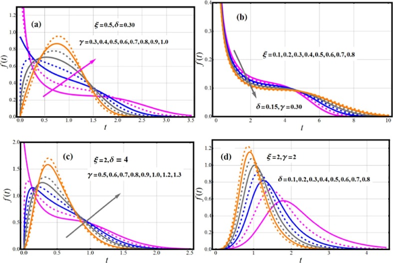
Depending on the parameter values, the EOWR density functions can take on a variety of structures (see Fig. 1 ). The PDF's possible shapes according to the parameter $\xi ,\gamma$ that regulates the distribution's shape, also the parameter $\delta$ which determine the scale of the distribution, like, uni-modal, decreasing, symmetric, inverted J and asymmetric forms (Fig. 1(a-d)). The failure function (FF) function is shown in Fig. 2 . This shows monotonic increasing behavior under considered parametric values.

Fig. 1.

Impact of parametric vector on PDF of EOWR model.

Fig. 2.

Impact of Parametric vector on FF of EOWR model.

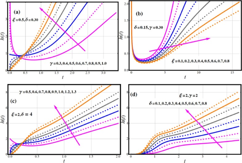
Fig. 4 demonstrates shapes of failure/hazard rate function (FRF/ HRF) function. The different forms of FRF/ HRF are predicted, which include decreasing, Uni-modal, increasing, upside down curve, and bathtub shapes which are all desirable qualities in a lifetime model. These versatile FRF forms are excellent for including monotonic (MNT) and non-monotonic (NMNT) hazard rate trends that are generally typical in real applications.

Fig. 4.

Impact of parametric vector on HRF of EOWR model.

The EOWR distribution is widely used in domains like biomedical investigations, biology, dependability, physical engineering, and survival study because of its versatility and ability to replicate skewed data.

Survival metrics

The goal of survival analysis, also known as reliability analysis in engineering, is to establish a link between variables and an event's time. The term “survival analysis” comes from clinical research, in which forecasting the time to death, or “survival,” is frequently the primary goal. One of the most used statistical techniques for assessing data on time to an event like device failure, heart attack and death so on is survival analysis. Many aspects of legal procedures require such data analysis, including apportioning coming medical care bills, assessing the number of years of life lost, assessing the product's dependability, examining the safety of pharmaceuticals, gauging the feasibility of medical therapies and equipment, calculating actuarial loss, and so on.

Survival function

The survival metric is an equation that can be used to calculate the chances of living to a certain age. Despite the fact that much of scientific research employs mathematical equations to calculate the survival metric, actuaries have typically relied on tables that calculate likelihood of surviving a year based on an individual's age and gender. Plots depicting the proportion of the population alive after a set length of time are often utilized. Risk factors are attributes that may raise probability of death, like blood pressure, lifestyle, smoking status, heredity, and environment. However, it is imperative not to overlook elements that boost survival chances. Lifestyle, social condition (i.e., married), and other factors are among them. Let T be a random variable that indicates an individual's lifespan. The survival function $\stackrel{⌣}{S}\left(\left(t\right|\xi ,\gamma ,\delta \right)$ of EOWR is.

$$R\left(\left(t\right|\xi ,\gamma ,\delta \right)={\left\{1+\xi {\left[e^{\delta t^2}-1\right]}^{\gamma }\right\}}^{-\frac{1}{\xi }},t,\delta ,\xi ,\gamma >0.$$ (3)

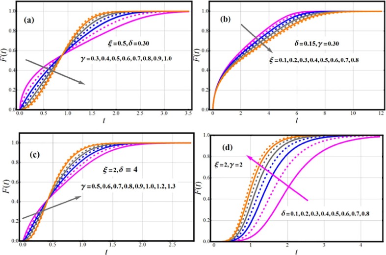
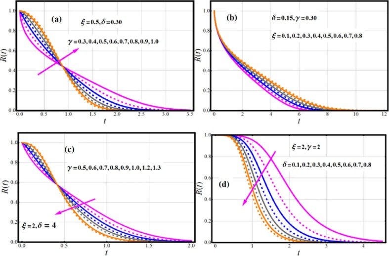
The survivability metric is a continuous monotonic decreasing function with $\underset{t\to -\infty }{\lim }S\left(t\right)=1$ and $\underset{t\to \infty }{\lim }S\left(t\right)=0.$ The survivability of many individuals varies with the amount of time they have been in use. Fig. 3 shows graphs of EOWR model survival function for various parameter values.

Fig. 3.

Impact of Parametric vector on SF/RF of NLT-W model.

Hazard function

A lifetime distribution's hazard function is one of its most essential features. It shows how the risk of failure shifts or with age, which is useful in most applications. Model selection might be facilitated by prior knowledge about the hazard's shape. Furthermore, if factors affecting an individual's lifespan change over time, it's usually necessary to model using the hazard function.

The term “failure rate function” is routinely employed in the research. This concept is used to describe an individual's failure rate over a set period of time and is formally expressed as $h\left(\left(t\right|\xi ,\gamma ,\delta \right)=f\left(\left(t\right|\xi ,\gamma ,\delta \right)/\left[1-F\left(\left(t\right|\xi ,\gamma ,\delta \right)\right]$. Hazard functions describe the evolution of the failure rate over time. The failure rate function of EOWR model is.

$$h\left(\left(t\right|\xi ,\gamma ,\delta \right)=2\gamma \delta t{e}^{\delta t^2}{\left(e^{\delta t^2}-1\right)}^{\gamma -1}{\left\{1+\xi {\left[e^{\delta t^2}-1\right]}^{\gamma }\right\}}^{-1}$$ (4)

The higher the failure rate is, the faster the reliability drops with time.

Cumulative hazard rate function

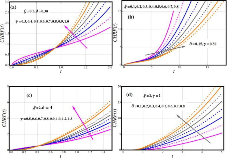
The cumulative hazard rate $\stackrel{⌣}{H}\left(\left(t\right|\xi ,\gamma ,\delta \right)$ is important in survival analyses. The cumulative hazard rate function (CHRF) or integrated hazard function of EOWR model is.

$$\stackrel{⌣}{H}\left(\left(t\right|\xi ,\gamma ,\delta \right)=\underset{0}{\overset{t}{\int }}\stackrel{⌣}{h}\left(\left(y\right|\xi ,\gamma ,\delta \right)dy=-\log \left\{\stackrel{⌣}{S}\left(\left(t\right|\xi ,\gamma ,\delta \right)\right\}.$$ (5)

Hence,

$$\stackrel{⌣}{H}\left(\left(t\right|\xi ,\gamma ,\delta \right)=\frac{1}{\xi }\log \left\{1+\xi {\left[e^{\delta t^2}-1\right]}^{\gamma }\right\}$$ (6)

Fig. 5 interprets the influence of the parameters on the EOWR cumulative hazard rate function profile. Monotonically increasing behavior is observed for chrf function of EOWR model.

Fig. 5.

Impact of Parametric vector on CHRF of EOWR model.

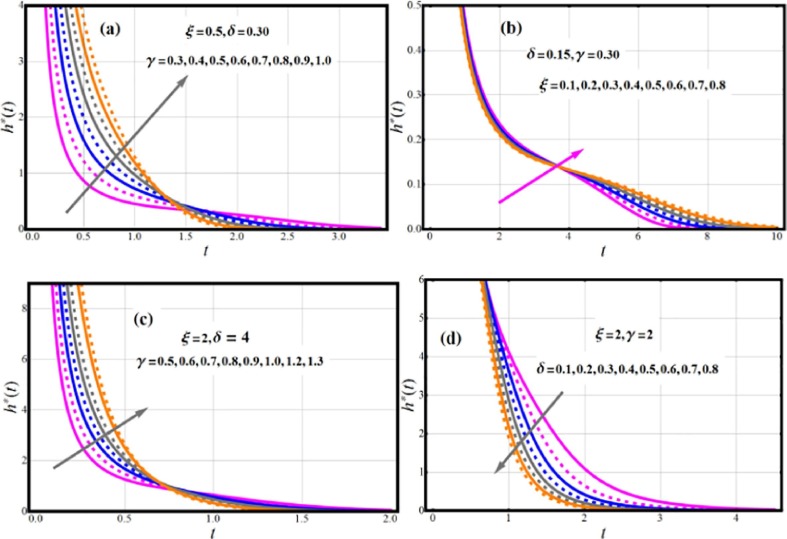
Reversed hazard rate function

The ratio of the PDF and the related CDF is characterized as the reversed hazard rate function (RHRF). The RHRF $\left(\stackrel{⌣}{h}\left(\left(t\right|\xi ,\gamma ,\delta \right)=f\left(\left(t\right|\xi ,\gamma ,\delta \right){\left[F\left(\left(t\right|\xi ,\gamma ,\delta \right)\right]}^{-1}\right)$ have recently grabbed experts' interest (see, for definitions, characterizations, and more information, Refs. [45], [46]).

$$\stackrel{⌣}{h}\left(\left(t\right|\xi ,\gamma ,\delta \right)=\frac{2\gamma \delta t{e}^{\delta t^2}{\left(e^{\delta t^2}-1\right)}^{\gamma -1}{\left\{1+\xi {\left[e^{\delta t^2}-1\right]}^{\gamma }\right\}}^{-\frac{\xi +1}{\xi }}}{1-{\left\{1+\xi {\left[e^{\delta t^2}-1\right]}^{\gamma }\right\}}^{-\frac{1}{\xi }}}.$$ (7)

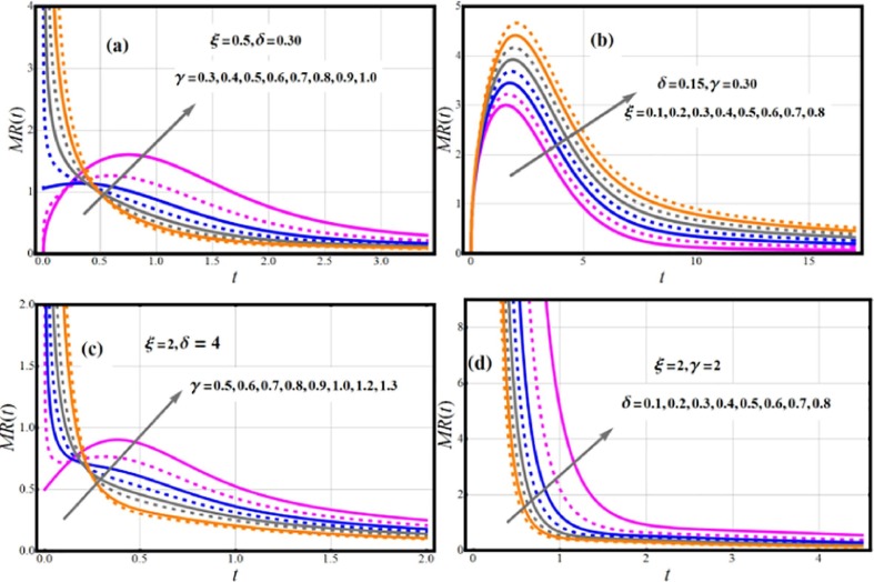
Mills Ratio

Because of its connection to failure rate, Mills Ratio (MR) is a unique technique for describing reliability.

$$MR\left(\left(t\right|\xi ,\gamma ,\delta \right)=\frac{S\left(\left(t\right|\xi ,\gamma ,\delta \right)}{f\left(\left(t\right|\xi ,\gamma ,\delta \right)}=\frac{\left\{1+\xi {\left[e^{\delta t^2}-1\right]}^{\gamma }\right\}}{2\gamma \delta t{e}^{\delta t^2}{\left(e^{\delta t^2}-1\right)}^{\gamma -1}}.$$ (8)

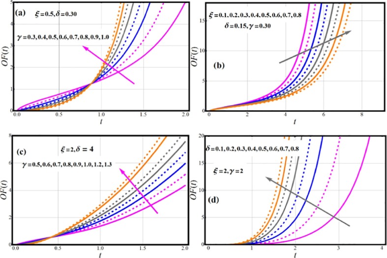
The odd function is defined by $\stackrel{⌣}{O}\left(\left(t\right|\xi ,\gamma ,\delta \right)=F\left(\left(t\right|\xi ,\gamma ,\delta \right)/S\left(\left(t\right|\xi ,\gamma ,\delta \right)$. The odd function of T is given by.

$$\stackrel{⌣}{O}\left(\left(t\right|\xi ,\gamma ,\delta \right)=\left[1-{\left\{1+\xi {\left[e^{\delta t^2}-1\right]}^{\gamma }\right\}}^{-\frac{1}{\xi }}\right]{\left\{1+\xi {\left[e^{\delta t^2}-1\right]}^{\gamma }\right\}}^{\frac{1}{\xi }}.$$ (9)

Depending on the parameter values, the EOWR density functions can take on a variety of structures (see The RHRF is shown in Fig. 6 . This shows monotonic decreasing behavior under considered parametric values. Fig. 7 demonstrates shapes of MR. The different forms of MR are predicted, which include decreasing, Uni-modal and upside down curve which are all desirable qualities in a lifetime model. These versatile MR forms are excellent for including monotonic (MNT) and non-monotonic (NMNT) hazard rate trends that are generally typical in real applications. Fig. 8 interprets the influence of the parameters on the EOWR odd function profile. Monotonically increasing behavior is observed for odd function of EOWR model.

Fig. 6.

Impact of Parametric vector on RHRF of EOWR model.

Fig. 7.

Impact of Parametric vector on MR of EOWR model.

Fig. 8.

Impact of Parametric vector on OF of EOWR model.

Estimation technique

In the research, several methods for parameter estimate have been developed; however, the maximum likelihood technique is the most popular. The maximum likelihood estimator $\stackrel{⌣}{\mathrm{\Theta }}$ of $\mathrm{\Theta }$ is a function of the observed data that maximizes L (.) over all possible values of $\mathrm{\Theta }$ in the parameter space $\mathrm{\Theta }$. As a result, we only evaluate maximum likelihood estimation of EOWR’s unknown parameters from complete samples. Let $T_1,T_2,...,T_n$ be a random sample and related observed values, $t_1,t_2,...,t_n$ from EOWR model with parameter vector $\mathrm{\Theta }=\left(\xi ,\gamma ,\delta \right)$. The log-likelihood (log L (.)) is generally easier to maximize. Hence the log-likelihood of the joint probability function of $T_1,T_2,...,T_n$ is.

$$l\left(\left(\mathbf{t}\right|\xi ,\gamma ,\delta \right)=\log \prod _{i=1}^{n}f\left(t_i;\xi ,\gamma ,\delta \right).$$ (10)

$$\begin{array}{c}l\left(\left(\mathbf{t}\right|\xi ,\gamma ,\delta \right)\propto n\log \gamma +n\log \delta +\delta \sum _{i=1}^n{t}_i^2+\left(\gamma -1\right)\sum _{i=1}^n\log \left(e^{\delta t_i^2}-1\right)\\ -\left(\frac{\xi +1}{\xi }\right)\sum _{i=1}^n\log \left\{1+\xi {\left[e^{\delta t_i^2}-1\right]}^{\gamma }\right\}.\end{array}$$ (11)

We are now focused about getting the MLEs. To do so, we then maximize Eq. (11) and then compute partial derivatives with regard to unspecified parameters $\mathrm{\Theta }=\left(\xi ,\gamma ,\delta \right)$ and equate to zero, accordingly. The score function $U\left(.\right)$ is derivative of log L (.), the score vector components are.

$$U\left(\xi ,\gamma ,\delta \right)={\left[\frac{\partial l\left(\left(\mathbf{t}\right|\xi ,\gamma ,\delta \right)}{\partial \xi },\frac{\partial l\left(\left(\mathbf{t}\right|\xi ,\gamma ,\delta \right)}{\partial \gamma },\frac{\partial l\left(\left(\mathbf{t}\right|\xi ,\gamma ,\delta \right)}{\partial \delta }\right]}^T.$$ (12)

The following are partial derivatives w.r.t. $\xi ,\gamma \text{and}\delta$ respectively.

$$\frac{\partial l\left(\left(\mathbf{t}\right|\xi ,\gamma ,\delta \right)}{\partial \xi }=\frac{1}{{\xi }^2}\sum _{i=1}^n\log \left\{1+\xi {\left[e^{\delta t_i^2}-1\right]}^{\gamma }\right\}-\left(\frac{\xi +1}{\xi }\right)\sum _{i=1}^n\frac{{\left[e^{\delta t_i^2}-1\right]}^{\gamma }}{\left\{1+\xi {\left[e^{\delta t_i^2}-1\right]}^{\gamma }\right\}},$$ (13)

$$\frac{\partial l\left(\left(\mathbf{t}\right|\xi ,\gamma ,\delta \right)}{\partial \gamma }=\frac{n}{\gamma }+\frac{1}{{\xi }^2}\sum _{i=1}^n\log \left(e^{\delta t_i^2}-1\right)-\left(\xi +1\right)\sum _{i=1}^n\frac{{\left[e^{\delta t_i^2}-1\right]}^{\gamma }\log \left[e^{\delta t_i^2}-1\right]}{\left\{1+\xi {\left[e^{\delta t_i^2}-1\right]}^{\gamma }\right\}},$$ (14)

$$\frac{\partial l\left(\left(\mathbf{t}\right|\xi ,\gamma ,\delta \right)}{\partial \delta }=\frac{n}{\delta }+\sum _{i=1}^n{t}_i^2+\left(\gamma -1\right)\sum _{i=1}^n\frac{t_i^2{e}^{\delta t_i^2}}{\left(e^{\delta t_i^2}-1\right)}-\gamma \left(\xi +1\right)\sum _{i=1}^n\frac{{\left[e^{\delta t_i^2}-1\right]}^{\gamma -1}{t}_i^2{e}^{\delta t_i^2}}{\left\{1+\xi {\left[e^{\delta t_i^2}-1\right]}^{\gamma }\right\}}.$$ (15)

The exact solutions for MLEs and optimal value of $\xi ,\gamma \text{and}\delta$ are not obtained by the last three non-linear equations. In these kinds of ML estimates, the Newton-Raphson (appropriate) algorithm is helpful.

ANN model design

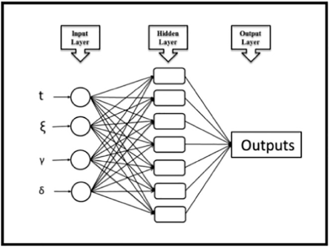
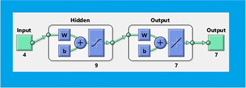
A multilayer perceptron (MLP) ANN model was designed to estimate survival metrics. MLP network models are one of the routinely recommended neural network models with ideal output behavior thanks to their strong structures and learning algorithms [47], [48], [49]. In the ANN model's input information layer, 4 different input parameters, namely mortality rate, two separate shape parameters and scale parameters, were determined and 7 different survival metrics were estimated in the output layer. Fig. 9 depicts the fundamental design of the constructed MLP network. There is no approach for exhibiting the component of computation named neuron in the hidden layer of MLP networks [50], [51], [52]. For this reason, the method used in the literature was followed and the performance of neural network models designed having various amounts of neurons was examined. After comparative study, the model with 9 neurons in hidden layer was decided. The basic architectural structure of designed neural network is presented in Fig. 10 . Data optimization and suitable grouping set employed in the progression of ANN models is one of the hyperparameters which directly affects prediction behavior of the model [53]. 70% of the data employed in the MLP network designed with a total of 59 datasets are grouped for training model, 15% for the confirmation phase and 15% for the testing phase [54], [55], [56]. In the hidden and output layers of the neural network, Tan-Sig and Purelin transfer functions are utilized respectively. The transfer functions [57] are:

$$f(x)=\frac{1}{1+\exp (-x)}$$ (16)

$$\text{purelin}\left(\text{x}\right)=x$$ (17)

Fig. 9.

The fundamental design of the established MLP network.

Fig. 10.

The basic architectural structure of the designed neural network.

Another hyper parameter that affects the training and learning capabilities of neural networks is the training algorithms [58]. Levenberg-Marquardt training algorithm, which is one of the algorithms with deep learning and training performance, is employed in designed neural network model [59]. After the development of the MLP network, the training, learning and prediction accuracies of the network model were examined and verified. For this purpose, coefficient of determination (R), Mean Squared Error (MSE) and proportional deviation values, which are widely used in the research, were used [60]. The mathematical expressions utilized in assessing of the efficiency characteristics [61] are:

$$\mathit{MSE}=\frac{1}{N}\sum _{i=1}^N{\left(X_{\text{targ}\left(i\right)}-X_{\text{pred}\left(i\right)}\right)}^2$$ (18)

$$R=\sqrt{1-\sum _{i=1}^N{\left(X_{\text{targ}\left(i\right)}-X_{\text{pred}\left(i\right)}\right)}^2{\left\{\sum _{i=1}^N{\left(X_{\text{targ}\left(i\right)}\right)}^2\right\}}^{-1}}$$ (19)

$$\mathit{Deviation}\left(\%\right)=[\frac{X_{t\arg }-X_{\mathit{pred}}}{X_{t\arg }}]\times 100$$ (20)

Validation of maximum likelihood method and ANN predict

In this part, we examine the implementation EOWR model for data of biological sciences. This data set is studied in detail by Almongy et al. [39]. They studied the 59-day mortality rates in Italy, which were observed between February 27 and April 27, 2020.

The results of this study revealed that when the EOWR model was compared to competing models such as Rayleigh, Kumaraswamy exponentiated Rayleigh, extended odd Weibull exponential, and Marshall-Olkin Rayleigh models, the Anderson–Darling, Crammervon Mises, and Kolmogorov–Smirnov (KS) statistic and its P-value were used as criteria for model selection, the EOWR's implementation meets all of the criteria for a better fit model. The results of their studies regarding the MLEs of parameters for the mortality rates data results are $\stackrel{⌢}{\gamma }=2.9019,\stackrel{⌢}{\xi }=15.8688\text{and}\stackrel{⌢}{\delta }=0.0551.$

We have now achieved numerical results utilizing these results that evaluated the effects of maximum likelihood estimates of pertinent parameters on the FF, RF, HRF, RHRF, Mills Ratio, odd function, and CHRF for mortality rates data and predict these outcomes using an ANN model. These values of the survival metrics of interest were calculated for the purpose of determining the accuracy of the results for the $\stackrel{⌢}{\gamma }=2.9019,\stackrel{⌢}{\xi }=15.8688\text{and}\stackrel{⌢}{\delta }=0.0551.$

The performance of the FF, RF, HRF, RHRF, Mills Ratio, Odd function, and CHRF for mortality rates data derived from numerical estimation using the Maximum Likelihood approach and ANN prediction. When compared to the ANN model, these have been shown to be in good agreement. As a result, it can be concluded that the current study can be used reliably to investigate these research issue.

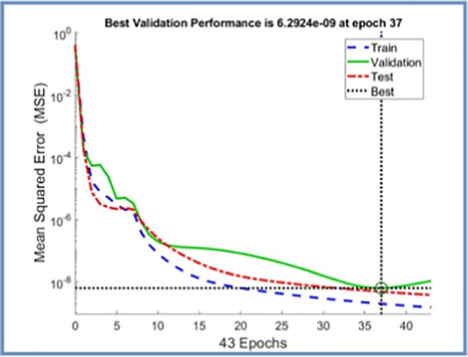
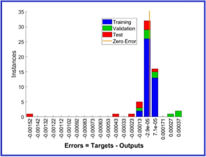
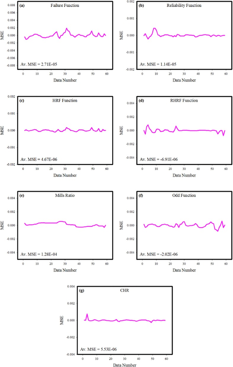
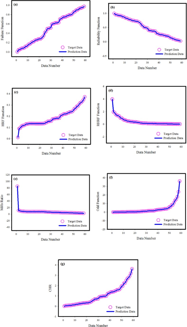
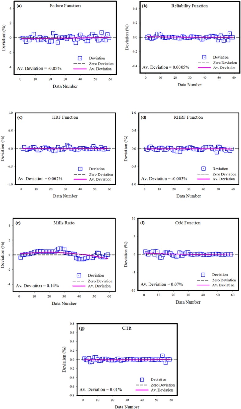
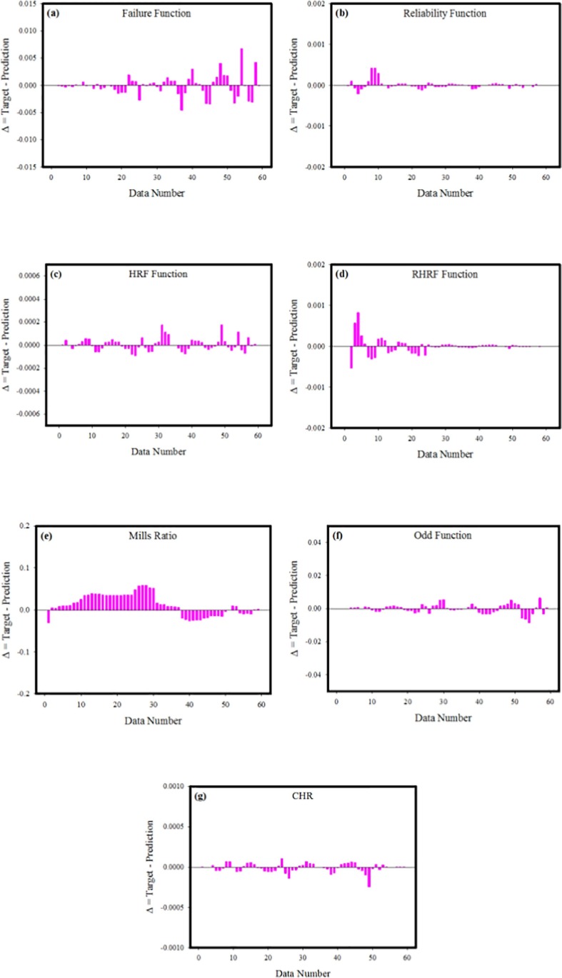
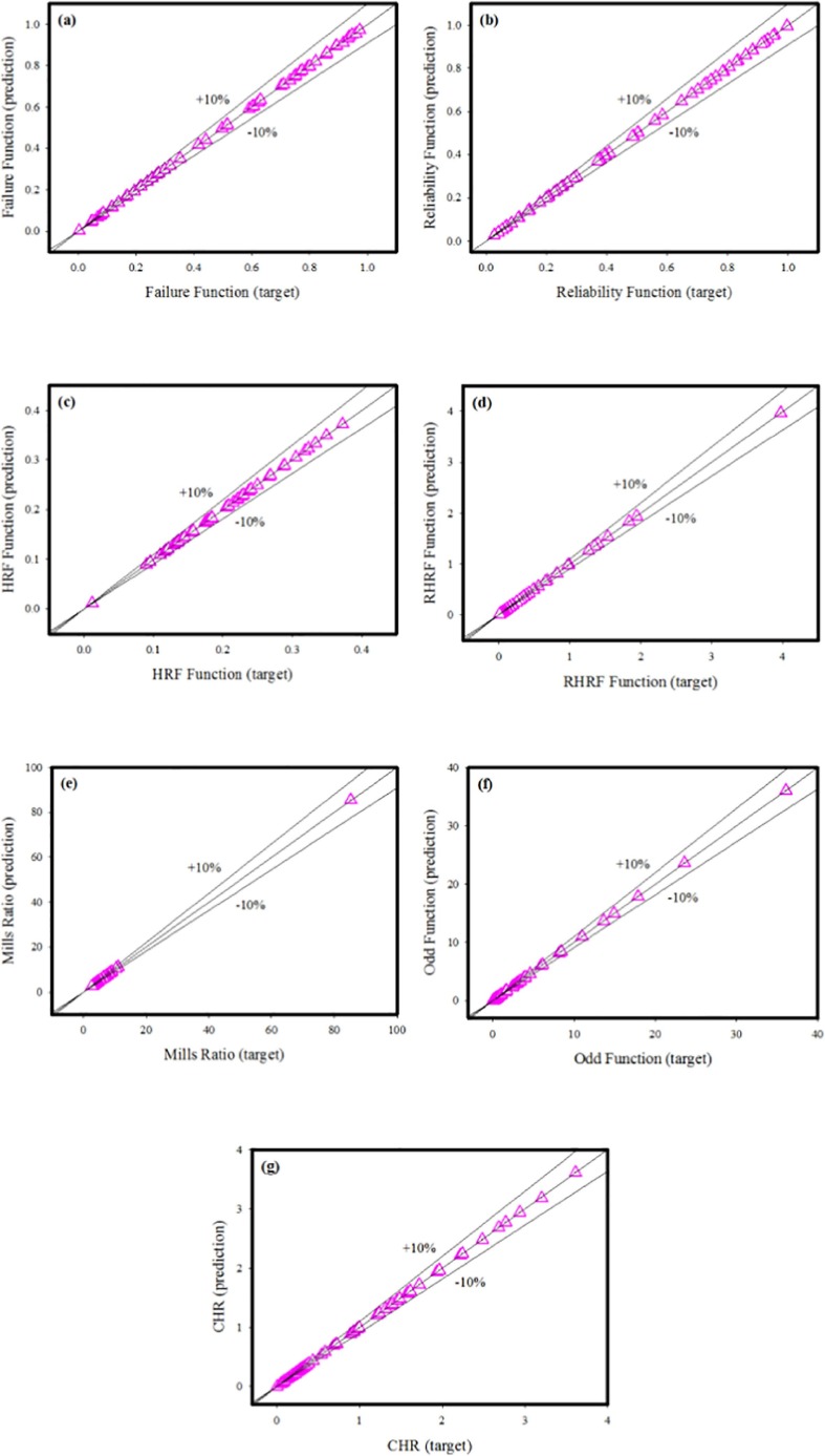
Ensuring the training and learning reliability of the developed ANN model is vital step in verifying the prediction behavior of the model. In Fig. 11 , the training performance of designed neural network is given. It is apparent to notice from the figure that the MSE values, which are high in the initial phase, diminish with the advancing epochs. The fact that MSE values approach zero represents that the errors acquired from the training phase of the neural network are also decreasing. The point where the MSE values acquired from the training, validation and testing phases intersect with best validation line is the point where the most ideal training data has been reached, and training phase of the model has been terminated at this stage. The differences between the outputs acquired during training phase of ANN model and the target data are shown in error histogram given in Fig. 12 . When the results obtained from the error histograms are scrutinized, the disparities between the target values and the simulated values are extremely small, as can be observed. It should also be noted that the errors are integrated near the zero error line, which is generally drawn in yellow. These findings obtained from the error histogram confirm that the training phase of the developed neural network was completed with very low errors. Fig. 13 shows MSE values calculated for each of the 59 data used in training the neural network. When MSE values presented separately for each output value are examined, it is seen that MSE values are generally very close to the zero error line. The closeness of the MSE values to the zero error line shows that the calculated MSE values for each data point are very close to zero. These low values of MSE values confirm that the developed ANN model completed the training and learning stages with very low errors and learned the relationship between the data in a very ideal way. In order to analyze the prediction accuracy of MLP network model, the outputs obtained from the neural network and the target data for each of the 7 different output values are shown on the same figure. When the graphs presented in Fig. 14 are scrutinized, it will be seen that the simulation outputs shown with blue lines are in perfect agreement with the target values expressed with red circles. This ideal fit of the simulation results with the target data confirms that the developed ANN model can predict each output value with very high accuracy. Evaluation of the proportional deviation between the outputs obtained from the neural network and the target data is important in analyzing the prediction errors of the neural network. In Fig. 15 , the proportional deviation values evaluated for each data are given. Looking at the deviation results expressed with blue squares, it can be observed that they are almost close near to zero error line for each output. When the mean deviation line expressed with the red line is examined, it is clearly seen that it has a very similar trend with the zero error line. The results produced from the deviation values prove that designed MLP network can predict with very low errors. In order to study error rates of the designed MLP neural networks more comprehensively, for each of the 7 output values, the deviations between the target data and output values at each data point are calculated and shown in Fig. 16 . When the lines expressing the difference values are evaluated, it is seen that the deviations calculated for each data are very low. The low differences between the target data and the prediction values show that prediction values acquired from the ANN model are the readings are fairly close to the target values. This is another indication that neural network is developed to have very low prediction errors. Because to understand the prediction reliability of the neural network in more detail, target data are put on the x-axis of Fig. 17 , and simulation outputs are put on the y-axis and the data points' positions are studied. When the data points obtained for 7 output values are assessed, it is observed that each point is located on the zero error line. The fact that data points are located close to zero error line shows that the predicted values and target values are in perfect line with each another. The obtained outcomes clearly confirm that developed ANN model can predict with very high correctness and very low errors.

Fig. 11.

The training performance of the designed neural network.

Fig. 12.

Error histogram for the designed ANN model.

Fig. 13.

The MSE values calculated for each of the 59 data used in training the neural network.

Fig. 14.

The responses acquired from the neural network and the target data.

Fig. 15.

The proportional deviation values calculated for each data.

Fig. 16.

The deviations between the target data and the output readings at each data point.

Fig. 17.

Target and prediction values for all outputs.

Conclusions

This article discussed the uses of the maximum likelihood technique and ANN modelling. This work investigates the applicability of ANN models in a study of COVID-19 mortality rates. The survival metrics of the EOWR model have been evaluated using seven different measures. The numerical approach of estimate has been used to calculate the survival characters to be evaluated. ANNs have been demonstrated to be useful in survival analysis as generic non-linear models. The current study has been comprised of comparative analysis of maximum likelihood method and ANN model of new lifetime EOWR model. As generic non-linear models, ANNs have been shown to be beneficial in survival analysis. The current research included a comparison of the maximum likelihood approach and the ANN model of a new lifespan EOWR model. This novel model has been used with survival based analysis of data of mortality rate of COVID-19. The training, learning and prediction performance of the developed ANN model has been extensively studied and evaluated. The maximum deviation between the estimation values obtained from the ANN model and the target data was found to be −0.14%. Another performance parameter, the R value, was calculated as 0.99836. The findings revealed that the ANN model provides high accuracy prediction and optimization results. The study also demonstrated that ANNs are an excellent engineering tool for predicting survival and mortality rates.

CRediT authorship contribution statement

Anum Shafiq: Conceptualization, Writing – review & editing, Data curation, Formal analysis, Methodology, Validation. Andaç Batur Çolak: Conceptualization, Software, Writing – review & editing, Data curation, Formal analysis, Methodology, Validation. Tabassum Naz Sindhu: Conceptualization, Methodology, Writing – original draft, Data curation, Formal analysis, Validation, Conceptualization. Showkat Ahmad Lone: Formal analysis, Writing – original draft, Data curation, Methodology, Validation. Abdelaziz Alsubie: Visualization, Writing – review & editing, Formal analysis, Methodology. Fahd Jarad: Supervision, Writing – review & editing.

Declaration of Competing Interest

The authors declare that they have no known competing financial interests or personal relationships that could have appeared to influence the work reported in this paper.

References

- 1.Zhao, J., Ahmad, Z., Almaspoor, Z., El-Morshedy, M., & Afify, A. Z. (2021). Modeling COVID-19 pandemic dynamics in two Asian countries. Computers, Materials and Continua, 965-977.
- 2.Alghamdi M., Alqarni M.S., Alshomrani A.S., Ullah M.Z., Baleanu D. Dynamics of COVID-19 via singular and non-singular fractional operators under real statistical observations. Mathemat Methods Appl Sci. 2020 [Google Scholar]
- 3.Anastassopoulou C., Russo L., Tsakris A., Siettos C., Othumpangat S. Data-based analysis, modelling and forecasting of the COVID-19 outbreak. PLoS ONE. 2020;15(3):e0230405. doi: 10.1371/journal.pone.0230405. [DOI] [PMC free article] [PubMed] [Google Scholar]
- 4.Langemann D., Nesteruk I., Prestin J. Comparison of mathematical models for the dynamics of the Chernivtsi children disease. Math Comput Simul. 2016;123:68–79. [Google Scholar]
- 5.Giordano, G., Blanchini, F., Bruno, R., Colaneri, P., Di Filippo, A., Di Matteo, A., & Colaneri, M. (2020). A SIDARTHE model of COVID-19 epidemic in Italy. arXiv preprint arXiv:2003.09861. [DOI] [PMC free article] [PubMed]
- 6.Naik P.A., Yavuz M., Qureshi S., Zu J., Townley S. Modeling and analysis of COVID-19 epidemics with treatment in fractional derivatives using real data from Pakistan. Eur Phys J Plus. 2020;135(10):1–42. doi: 10.1140/epjp/s13360-020-00819-5. [DOI] [PMC free article] [PubMed] [Google Scholar]
- 7.Musa S.S., Qureshi S., Zhao S., Yusuf A., Mustapha U.T., He D. Mathematical modeling of COVID-19 epidemic with effect of awareness programs. Infect Dis Modell. 2021;6:448–460. doi: 10.1016/j.idm.2021.01.012. [DOI] [PMC free article] [PubMed] [Google Scholar]
- 8.Atangana A., İğret Araz S. Modeling and forecasting the spread of COVID-19 with stochastic and deterministic approaches: Africa and Europe. Adv Diff Equat. 2021;2021(1):1–107. doi: 10.1186/s13662-021-03213-2. [DOI] [PMC free article] [PubMed] [Google Scholar]
- 9.Hassan A.S., Almetwally E.M., Ibrahim G.M. Kumaraswamy inverted topp-leone distribution with applications to COVID-19 data. Comput Mater Continua. 2021:337–358. [Google Scholar]
- 10.Shafiq A., Lone S.A., Sindhu T.N., El Khatib Y., Al-Mdallal Q.M., Muhammad T. A new modified Kies Fréchet distribution: applications of mortality rate of Covid-19. Results Phys. 2021;28:104638. doi: 10.1016/j.rinp.2021.104638. [DOI] [PMC free article] [PubMed] [Google Scholar]
- 11.Atangana A., araz S.İĞret. A novel Covid-19 model with fractional differential operators with singular and non-singular kernels: analysis and numerical scheme based on Newton polynomial. Alexand Eng J. 2021;60(4):3781–3806. [Google Scholar]
- 12.Ibrahim G.M., Hassan A.S., Almetwally E.M., Almongy H.M. Parameter estimation of alpha power inverted Topp-Leone distribution with applications. Intell Autom Soft Comput. 2021;29:353–371. [Google Scholar]
- 13.Nesteruk I. Comparison of the coronavirus pandemic dynamics in Ukraine and neighboring countries. Preprint] ResearchGate. 2020 [Google Scholar]
- 14.Nadler, P., Arcucci, R., & Guo, Y. (2020, November). A neural sir model for global forecasting. In Machine Learning for Health (pp. 254-266). PMLR.
- 15.Kuniya T. Prediction of the epidemic peak of coronavirus disease in Japan, 2020. J Clin Med. 2020;9(3):789. doi: 10.3390/jcm9030789. [DOI] [PMC free article] [PubMed] [Google Scholar]
- 16.Dandekar, R., & Barbastathis, G. (2020). Neural Network aided quarantine control model estimation of global Covid-19 spread. arXiv preprint arXiv:2004.02752.
- 17.Anderez D.O., Kanjo E., Pogrebna G., Kaiwartya O., Johnson S.D., Hunt J.A. A COVID-19-based modified epidemiological model and technological approaches to help vulnerable individuals emerge from the lockdown in the UK. Sensors. 2020;20(17):4967. doi: 10.3390/s20174967. [DOI] [PMC free article] [PubMed] [Google Scholar]
- 18.Huang Y., Yang L., Dai H., Tian F., Chen K. Epidemic situation and forecasting of COVID-19 in and outside China. Bull World Health Organ. 2020;10 [Google Scholar]
- 19.Kheirallah K.A., Alsinglawi B., Alzoubi A., Saidan M.N., Mubin O., Alorjani M.S., et al. The effect of strict state measures on the epidemiologic curve of COVID-19 infection in the context of a developing country: a simulation from Jordan. Int J Environ Res Public Health. 2020;17(18):6530. doi: 10.3390/ijerph17186530. [DOI] [PMC free article] [PubMed] [Google Scholar]
- 20.Sun D., Duan L., Xiong J., Wang D. Modeling and forecasting the spread tendency of the COVID-19 in China. Adv Diff Equat. 2020;2020(1):1–16. doi: 10.1186/s13662-020-02940-2. [DOI] [PMC free article] [PubMed] [Google Scholar]
- 21.Alzaatreh A., Lee C., Famoye F. A new method for generating families of continuous distributions. Metron. 2013;71(1):63–79. [Google Scholar]
- 22.Cordeiro G.M., Alizadeh M., Silva R.B., Ramires T.G. A new wider family of continuous models: the extended cordeiro and de castro family. Hacettepe J Mathemat Statist. 2017;47(4):937–961. [Google Scholar]
- 23.Abouammoh A., Kayid M. A new family of extended Lindley models: Properties, estimation and applications. Mathematics. 2020;8(12):2146. [Google Scholar]
- 24.Mansour M.M., Ibrahim M., Aidi K., Shafique Butt N., Ali M.M., Yousof H.M., et al. A new log-logistic lifetime model with mathematical properties, copula, modified goodness-of-fit test for validation and real data modeling. Mathematics. 2020;8(9):1508. [Google Scholar]
- 25.Tahir M.H., Hussain M.A., Cordeiro G.M. A new flexible generalized family for constructing many families of distributions. J Appl Statis. 2021:1–21. doi: 10.1080/02664763.2021.1874891. [DOI] [PMC free article] [PubMed] [Google Scholar]
- 26.Maurya S.K., Nadarajah S. Poisson generated family of distributions: a review. Sankhya B. 2021;83(2):484–540. [Google Scholar]
- 27.Chen Z. A new two-parameter lifetime distribution with bathtub shape or increasing failure rate function. Statist Probab Lett. 2000;49(2):155–161. [Google Scholar]
- 28.Kumar S. Monitoring novel corona virus (COVID-19) infections in India by cluster analysis. Ann Data Sci. 2020;7(3):417–425. doi: 10.1007/s40745-020-00289-7. [DOI] [PMC free article] [PubMed] [Google Scholar]
- 29.Khakharia A., Shah V., Jain S., Shah J., Tiwari A., Daphal P., et al. Outbreak prediction of COVID-19 for dense and populated countries using machine learning. Ann Data Sci. 2021;8(1):1–19. doi: 10.1007/s40745-020-00314-9. [DOI] [PMC free article] [PubMed] [Google Scholar]
- 30.Sindhu T.N., Shafiq A., Al-Mdallal Q.M. Exponentiated transformation of gumbel type-II distribution for modeling COVID-19 data. Alexand Eng J. 2021;60(1):671–689. [Google Scholar]
- 31.Sindhu T.N., Shafiq A., Al-Mdallal Q.M. On the analysis of number of deaths due to Covid− 19 outbreak data using a new class of distributions. Results Phys. 2021;21:103747. doi: 10.1016/j.rinp.2020.103747. [DOI] [PMC free article] [PubMed] [Google Scholar]
- 32.Sindhu T.N., Hussain Z., Alotaibi N., Muhammad T. Estimation method of mixture distribution and modeling of COVID-19 pandemic. AIMS Mathemat. 2022;7(6):9926–9956. [Google Scholar]
- 33.Wáng Y.X.J. A call for caution in extrapolating chest CT sensitivity for COVID-19 derived from hospital data to patients among general population. Quant Imag Med Surg. 2020;10(3):798–799. doi: 10.21037/qims.2020.03.04. [DOI] [PMC free article] [PubMed] [Google Scholar]
- 34.Lalmuanawma S., Hussain J., Chhakchhuak L. Applications of machine learning and artificial intelligence for Covid-19 (SARS-CoV-2) pandemic: a review. Chaos, Solitons Fractals. 2020;139:110059. doi: 10.1016/j.chaos.2020.110059. [DOI] [PMC free article] [PubMed] [Google Scholar]
- 35.Lone, S. A., Sindhu, T. N., & Jarad, F. (2021). Additive Trinomial Fréchet distribution with practical application. Results in Physics, 105087. [DOI] [PMC free article] [PubMed]
- 36.Lone S.A., Sindhu T.N., Shafiq A., Jarad F. A novel extended Gumbel Type II model with statistical inference and Covid-19 applications. Results Phys. 2022;35:105377. doi: 10.1016/j.rinp.2022.105398. [DOI] [PMC free article] [PubMed] [Google Scholar]
- 37.Shafiq A., Sindhu T.N., Alotaibi N. A novel extended model with versatile shaped failure rate: statistical inference with Covid-19 applications. Results Phys. 2022;36:105398. doi: 10.1016/j.rinp.2022.105398. [DOI] [PMC free article] [PubMed] [Google Scholar]
- 38.Bullock J., Luccioni A., Pham K.H., Lam C.S.N., Luengo-Oroz M. Mapping the landscape of artificial intelligence applications against COVID-19. J Artif Intell Res. 2020;69:807–845. [Google Scholar]
- 39.Almongy H.M., Almetwally E.M., Aljohani H.M., Alghamdi A.S., Hafez E.H. A new extended Rayleigh distribution with applications of COVID-19 data. Results Phys. 2021;23:104012. doi: 10.1016/j.rinp.2021.104012. [DOI] [PMC free article] [PubMed] [Google Scholar]
- 40.Ayyildiz E., Erdogan M., Taskin A. Forecasting COVID-19 recovered cases with Artificial Neural Networks to enable designing an effective blood supply chain. Comput Biol Med. 2021;139:105029. doi: 10.1016/j.compbiomed.2021.105029. [DOI] [PMC free article] [PubMed] [Google Scholar]
- 41.Kuvvetli Y., Deveci M., Paksoy T., Garg H. A predictive analytics model for COVID-19 pandemic using artificial neural networks. Decis Anal J. 2021;1:100007. [Google Scholar]
- 42.Kianfar N., Mesgari M.S., Mollalo A., Kaveh M. Spatio-temporal modeling of COVID-19 prevalence and mortality using artificial neural network algorithms. Spatial Spatio-Temp Epidemiol. 2022;40:100471. doi: 10.1016/j.sste.2021.100471. [DOI] [PMC free article] [PubMed] [Google Scholar]
- 43.Çolak A.B. (2021). Prediction of Infection and Death Ratio of COVID-19 Virus in Turkey by Using Artificial Neural Network (ANN), 2 (1), 106 – 112.
- 44.Alhasan M., Hasaneen M. Digital imaging, technologies and artificial intelligence applications during COVID-19 pandemic. Comput Med Imaging Graph. 2021;91:101933. doi: 10.1016/j.compmedimag.2021.101933. [DOI] [PMC free article] [PubMed] [Google Scholar]
- 45.Keilson J., Sumita U. Uniform stochastic ordering and related inequalities. Can J Statis. 1982;10(3):181–198. [Google Scholar]
- 46.Gupta R.D., Nanda A.K. Some results on reversed hazard rate ordering. Commun Statis Theory Methods. 2001;30(11):2447–2457. [Google Scholar]
- 47.Vaferi B., Samimi F., Pakgohar E., Mowla D. Artificial neural network approach for prediction of thermal behavior of nanofluids flowing through circular tubes. Powder Technol. 2014;267:1–10. [Google Scholar]
- 48.Canakci A., Ozsahin S., Varol T. Modeling the influence of a process control agent on the properties of metal matrix composite powders using artificial neural networks. Powder Technol. 2012;228:26–35. [Google Scholar]
- 49.Vaferi B., Eslamloueyan R., Ayatollahi S. Automatic recognition of oil reservoir models from well testing data by using multi-layer perceptron networks. J Petrol Sci Eng. 2011;77(3–4):254–262. [Google Scholar]
- 50.Ahmadloo E., Azizi S. Prediction of thermal conductivity of various nanofluids using artificial neural network. Int Commun Heat Mass Transfer. 2016;74:69–75. [Google Scholar]
- 51.Bonakdari H., Zaji A.H. Open channel junction velocity prediction by using a hybrid self-neuron adjustable artificial neural network. Flow Meas Instrum. 2016;49:46–51. [Google Scholar]
- 52.Çolak A.B., Güzel T., Yıldız O., Özer M. An experimental study on determination of the shottky diode current-voltage characteristic depending on temperature with artificial neural network. Physica B. 2021;608 [Google Scholar]
- 53.Çolak A.B. An experimental study on the comparative analysis of the effect of the number of data on the error rates of artificial neural networks. Int J Energy Res. 2021;45(1):478–500. [Google Scholar]
- 54.Esmaeilzadeh F., Teja A.S., Bakhtyari A. The thermal conductivity, viscosity, and cloud points of bentonite nanofluids with n-pentadecane as the base fluid. J Mol Liq. 2020;300:112307. [Google Scholar]
- 55.Barati-Harooni A., Najafi-Marghmaleki A. An accurate RBF-NN model for estimation of viscosity of nanofluids. J Mol Liq. 2016;224:580–588. [Google Scholar]
- 56.Shafiq A., Çolak A.B., Lone S.A., Sindhu T.N., Muhammad T. Reliability modeling and analysis of mixture of exponential distributions using artificial neural network. Mathemat Methods Appl Sci. 2022 [Google Scholar]
- 57.Akhgar A., Toghraie D., Sina N., Afrand M. Developing dissimilar artificial neural networks (ANNs) to prediction the thermal conductivity of MWCNT-TiO2/Water-ethylene glycol hybrid nanofluid. Powder Technol. 2019;355:602–610. [Google Scholar]
- 58.Ali A., Abdulrahman A., Garg S., Maqsood K., Murshid G. Application of artificial neural networks (ANN) for vapor-liquid-solid equilibrium prediction for CH4-CO2 binary mixture. Greenhouse Gases Sci Technol. 2019;9(1):67–78. [Google Scholar]
- 59.Abdul Kareem F.A., Shariff A.M., Ullah S., Garg S., Dreisbach F., Keong L.K., et al. Experimental and neural network modeling of partial uptake for a carbon dioxide/methane/water ternary mixture on 13X zeolite. Energy Technology. 2017;5(8):1373–1391. [Google Scholar]
- 60.Çolak A.B., Yıldız O., Bayrak M., Tezekici B.S. Experimental study for predicting the specific heat of water based Cu-Al2O3 hybrid nanofluid using artificial neural network and proposing new correlation. Int J Energy Res. 2020;44(9):7198–7215. [Google Scholar]
- 61.Kalkan O., Colak A.B., Celen A., Bakirci K., Dalkilic A.S. Prediction of experimental thermal performance of new designed cold plate for electric vehicles’ Li-ion pouch-type battery with artificial neural network. J Storage Mater. 2022;48:103981. [Google Scholar]