Improving Polygenic Prediction in Ancestrally Diverse Populations

Abstract

Polygenic risk scores (PRS) have attenuated cross-population predictive performance. As existing genome-wide association studies (GWAS) were predominantly conducted in individuals of European descent, the limited transferability of PRS reduces their clinical value in non-European populations and may exacerbate healthcare disparities. Recent efforts to level ancestry imbalance in genomic research have expanded the scale of non-European GWAS, although most of them remain underpowered. Here we present a novel PRS construction method, PRS-CSx, which improves cross-population polygenic prediction by integrating GWAS summary statistics from multiple populations. PRS-CSx couples genetic effects across populations via a shared continuous shrinkage prior, enabling more accurate effect size estimation by sharing information between summary statistics and leveraging linkage disequilibrium (LD) diversity across discovery samples, while inheriting computational efficiency and robustness from PRS-CS. We show that PRS-CSx outperforms alternative methods across traits with a wide range of genetic architectures, cross-population genetic overlaps and discovery GWAS sample sizes in simulations, and improves the prediction of quantitative traits and schizophrenia risk in non-European populations.

INTRODUCTION

Human complex traits and diseases are influenced by hundreds or thousands of genetic variants, each explaining a small proportion of phenotypic variation. Polygenic risk scores (PRS) aggregate genetic effects across the genome to measure the overall genetic liability to a trait or disease. PRS are not useful as a stand-alone diagnostic tool; rather, they have shown promise in predicting individualized disease risk and trajectories, stratifying patient groups, informing preventive, diagnostic and therapeutic strategies, and improving biomedical and health outcomes^1–6.

Despite the potential for clinical translation, recent theoretical and empirical studies showed that PRS have decreased cross-population prediction accuracy, especially when the discovery and target samples are genetically distant^7–10. As existing genome-wide association studies (GWAS) were predominantly conducted in individuals of European descent^11–14, the poor transferability of PRS across populations has impeded its clinical implementation and raised health disparity concerns⁷. Therefore, there is an urgent need to improve the accuracy of cross-population polygenic prediction in order to maximize the clinical potential of PRS and ensure equitable delivery of precision medicine to global populations.

As the efforts to diversify the samples in genomic research start to grow, the scale of non-European genomic resources has been expanded in recent years. Although the sample sizes of most non-European GWAS remain considerably smaller than European studies, they provide critical information on the variation of genetic effects across populations. Initial studies have indicated that the genetic architectures of many complex traits and diseases are largely concordant between populations – both at the single-variant level and at the genome-wide level^15–18, suggesting that the transferability of PRS may be improved by integrating GWAS summary statistics from diverse populations. However, current PRS construction methods have been designed primarily for applications within one homogeneous population^19–23. Existing methods that can take GWAS summary statistics from multiple populations use meta-analysis to summarize genetic effects across training datasets^24,25, but this approach does not model population-specific allele frequencies and linkage disequilibrium (LD) patterns. Alternatively, independent analysis can be performed on each discovery GWAS and the resulting PRS can be linearly combined^26,27, but this approach does not make full use of the genetic overlap between populations to inform PRS construction.

Here we present PRS-CSx, an extension of PRS-CS¹⁹, that improves cross-population polygenic prediction by jointly modeling GWAS summary statistics from multiple populations. We compare the predictive performance of PRS-CSx with existing PRS construction methods across traits with a wide range of genetic architectures, cross-population genetic overlaps, and discovery GWAS sample sizes via simulations. We further apply PRS-CSx to predict quantitative traits using data from the UK Biobank (UKBB)²⁸, Biobank Japan (BBJ)^29,30, the Population Architecture using Genomics and Epidemiology Consortium (PAGE) study³¹ and the Taiwan Biobank (TWB)^32,33, and predict schizophrenia risk using cohorts of European and East Asian ancestries^15,34.

RESULTS

Overview of PRS-CSx

PRS-CSx extends PRS-CS¹⁹, a recently developed Bayesian polygenic modeling and prediction framework, to improve cross-population polygenic prediction by integrating GWAS summary statistics from multiple ancestry groups (Methods). PRS-CSx uses a shared continuous shrinkage prior to couple SNP effects across populations, which enables more accurate effect size estimation by sharing information between summary statistics and leveraging LD diversity across discovery samples. The shared prior allows for correlated but varying effect size estimates across populations, retaining the flexibility of the modeling framework. In addition, PRS-CSx explicitly models population-specific allele frequencies and LD patterns, and inherits from PRS-CS the computational advantages of continuous shrinkage priors, and the efficient and robust posterior inference algorithm (Gibbs sampling). Given GWAS summary statistics and ancestry-matched LD reference panels, PRS-CSx calculates one polygenic score for each discovery sample, and integrates them by learning an optimal linear combination to produce the final PRS (Fig. 1).

Figure 1: Overview of polygenic prediction methods.

The predictive performances of three representative single-discovery methods: (i) LD-informed pruning and p-value thresholding (PT); (ii) LDpred2; (iii) PRS-CS; and five multi-discovery methods: (i) PT-meta; (ii) PT-mult; (iii) LDpred2-mult; (iv) PRS-CS-mult; (v) PRS-CSx are compared in this study. LDpred2-mult and PRS-CS-mult depicted here are not published methods but are helpful for comparing potential improvements from PRS-CSx that uses a coupled continuous shrinkage prior for the effect sizes of genetic variants. The discovery samples (to generate GWAS summary statistics), validation samples (to tune hyper-parameters in PRS construction methods) and testing samples (to assess prediction accuracy) are non-overlapping. LD ref: LD reference panel; pop A/B/C: Population A/B/C.

Overview of PRS analysis

We have broadly classified polygenic prediction methods into two categories: single-discovery methods, which train PRS using GWAS summary statistics from a single discovery sample; and multi-discovery methods, which combine GWAS summary statistics from multiple discovery samples for PRS construction. In this work, we assess and compare within- and cross-population predictive performance of three representative single-discovery methods: (i) LD-informed pruning and p-value thresholding (PT)³⁵; (ii) LDpred2²⁰; (iii) PRS-CS¹⁹; and four multi-discovery methods in addition to PRS-CSx: (i) PT-meta; (ii) PT-mult²⁶; (iii) LDpred2-mult; and (iv) PRS-CS-mult. PT-meta applies PT to the meta-analyzed discovery GWAS summary statistics. The three “mult” methods respectively apply PT, LDpred2 and PRS-CS to each discovery GWAS separately, and linearly combine the resulting PRS. PT-mult has been demonstrated to improve the prediction in recently admixed populations²⁶. Here we have extended the idea of PT-mult to LDpred2-mult and PRS-CS-mult, creating two new methods to quantify the benefits of jointly modeling multiple GWAS summary statistics via the coupled shrinkage prior. The workflow for each PRS construction method is shown in Fig. 1. In all the PRS analyses, we use the discovery dataset to estimate the marginal effect sizes of genetic variants and generate GWAS summary statistics for each population; we use the validation dataset, with individual-level genotypes and phenotypes, to tune hyper-parameters for different polygenic prediction methods; and we use the testing dataset, with individual-level genotypes and phenotypes, to evaluate the prediction accuracy of PRS and compute performance metrics using hyper-parameters learnt in the validation dataset. The three datasets comprise non-overlapping individuals. For convenience, we use the target dataset to refer to the combination of validation and testing datasets, which have matched ancestry. For fair comparison, we use 1000 Genomes Project (1KG) Phase 3³⁶ super-population samples (European N=503; East Asian N=504; African N=661; Admixed American N=347) as the LD reference panels across different PRS construction methods throughout the paper.

Simulations

We first evaluated the predictive performance of different polygenic prediction methods via simulations. We simulated individual-level genotypes of European (EUR), East Asian (EAS) and African (AFR) populations for HapMap3 variants with minor allele frequency (MAF) >1% in at least one of the three populations using HAPGEN2³⁷, with the 1KG Phase 3 samples as the reference panel. In our primary simulation setting, we randomly sampled 1% HapMap3 variants as causal variants, which in aggregation explained 50% of phenotypic variation in each population. We assumed that causal variants are shared across populations but allowed for varying effect sizes, which were sampled from a multivariate normal distribution with the cross-population genetic correlation (r_g) set to 0.7. The simulation was repeated 20 times.

We first applied single-discovery methods to GWAS summary statistics generated by 100K simulated EUR samples and 20K non-EUR (EAS or AFR) samples, and evaluated their predictive performance, measured by the squared correlation (R²) between the simulated and predicted phenotypes, in 20K target samples, which were evenly split into a validation dataset and a testing dataset (Fig. 2; Supplementary Table 1). As expected, when the target population was EUR, PRS trained on the larger EUR GWAS were substantially more accurate than PRS trained on non-EUR GWAS (Fig. 2; left panels). However, when the target population was EAS or AFR, PRS trained on ancestry-matched non-EUR GWAS were more predictive than EUR PRS (Fig. 2; right panels), even though the sample sizes of the non-EUR GWAS were much smaller (20K vs. 100K). Among the three single-discovery methods examined, Bayesian methods (LDpred2 and PRS-CS) consistently outperformed PT. PRS-CS appeared to be more accurate than LDpred2 in both within- and cross-population prediction when the discovery GWAS was well-powered, while LDpred2 was more accurate when the discovery sample size was limited, likely reflecting the strengths and limitations of the different priors used in PRS-CS and LDpred2 (Supplementary Note).

Figure 2: Prediction accuracy of single-discovery and multi-discovery polygenic prediction methods in simulations.

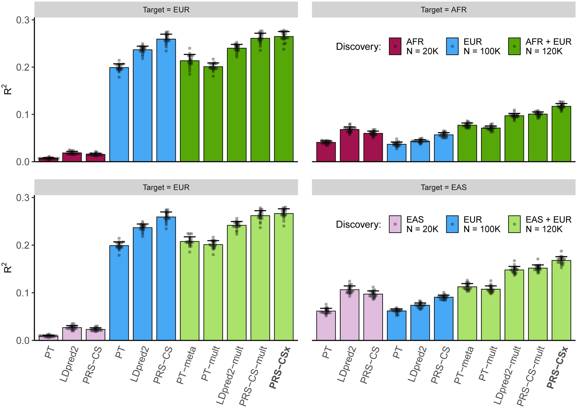
1% HapMap3 variants were randomly sampled as causal variants, which in aggregation explained 50% of phenotypic variation in each population. Causal variants were shared across populations with a cross-population genetic correlation of 0.7. 100K simulated EUR samples and 20K non-EUR (EAS or AFR) samples were used as the discovery dataset. Each bar shows the squared correlation (R²) between the simulated and predicted phenotypes for a polygenic prediction method in an independent testing dataset, averaged across 20 simulation replicates. Error bar indicates the standard deviation of R² across replicates. Prediction accuracy for each simulation replicate is overlaid on the bar plot.

We then assessed whether multi-discovery methods can improve cross-population polygenic prediction. Specifically, we used different multi-discovery methods to combine GWAS summary statistics from 100K EUR samples and 20K non-EUR (EAS or AFR) samples as the discovery dataset, and evaluated their predictive performance in independent target samples (Fig. 2; Supplementary Table 1). Figure 2 shows that, in general, multi-discovery methods improved prediction accuracy over their single-discovery counterparts (i.e., PT-meta or PT-mult vs. PT; LDpred2-mult vs. LDpred2; PRS-CS-mult vs. PRS-CS), reflecting the increase in discovery sample size. When the target population was EUR, the improvement of PRS-CSx and PRS-CS-mult over PRS-CS was marginal, suggesting that the benefits of adding a small non-EUR GWAS to the discovery dataset can be limited in this case. However, when predicting into non-EUR populations, multi-discovery methods clearly outperformed single-discovery methods, with Bayesian methods (LDpred2-mult, PRS-CS-mult and PRS-CSx) demonstrating a larger advantage over PT-based methods. PRS-CSx provided an additional increase of 10.6% and 16.4% in R² over PRS-CS-mult when the target population was EAS and AFR, respectively, demonstrating that joint modeling of the genetic architecture across populations using the coupled continuous shrinkage prior improves polygenic prediction in non-EUR populations.

We conducted a series of secondary simulations, by varying one parameter in the primary simulation at a time, to assess the generalizability of the above observations and the robustness of PRS-CSx across a wide range of genetic architectures, cross-population genetic overlaps and discovery GWAS sample sizes (Supplementary Note; Extended Data Figs. 1–7; Supplementary Tables 2–9). We concluded that, while the benefits of using a coupled prior varied with simulation designs and may be small in certain scenarios, PRS-CSx improved cross-population prediction accuracy relative to alternative methods across a vast majority of the simulation settings and was robust to model misspecification.

Prediction of quantitative traits in Biobanks

Next, we evaluated the predictive performance of different polygenic prediction methods using 33 anthropometric or blood panel traits from UKBB²⁸ (N=314,916–360,388) and BBJ³⁰ (N=71,221–165,419; Supplementary Table 10). All the 33 traits, with two exceptions (Basophil and Eosinophil), had moderate to high cross-population genetic-effect correlations estimated by POPCORN¹⁶ (range 0.37–0.85; Supplementary Table 10). We applied single-discovery methods to UKBB or BBJ summary statistics, and used multi-discovery methods to combine UKBB and BBJ GWAS. All target samples are unrelated UKBB individuals that are also unrelated with the UKBB discovery samples. We assigned each target sample to one of the five 1KG super-populations [AFR, AMR (Admixed American), EAS, EUR, SAS (South Asian)] (Methods), and assessed the prediction accuracy in each target population separately, adjusting for age, sex and top 20 principal components (PCs) of the genotypes. For each population, the target dataset was randomly and evenly split into a validation dataset and a testing dataset. The prediction accuracy, measured by variance explained (R²) in linear regression after adjusting for covariates, was averaged across 100 random splits.

Consistent with simulation results, Bayesian multi-discovery methods examined here (LDpred2-mult, PRS-CS-mult and PRS-CSx) often outperformed published single-discovery methods and PT-based multi-discovery methods, suggesting the importance of integrating available GWAS summary statistics and appropriately accounting for population-specific LD patterns in cross-population prediction (Fig. 3; Supplementary Table 11). The improvement of PRS-CSx in prediction accuracy relative to LDpred2 and PRS-CS trained on UKBB summary statistics (which on average were more accurate than PRS trained on BBJ GWAS), and LDpred2-mult and PRS-CS-mult (which were often the second and third best multi-discovery method) depended on the target population.

Figure 3: Relative prediction accuracy for quantitative traits within each target population.

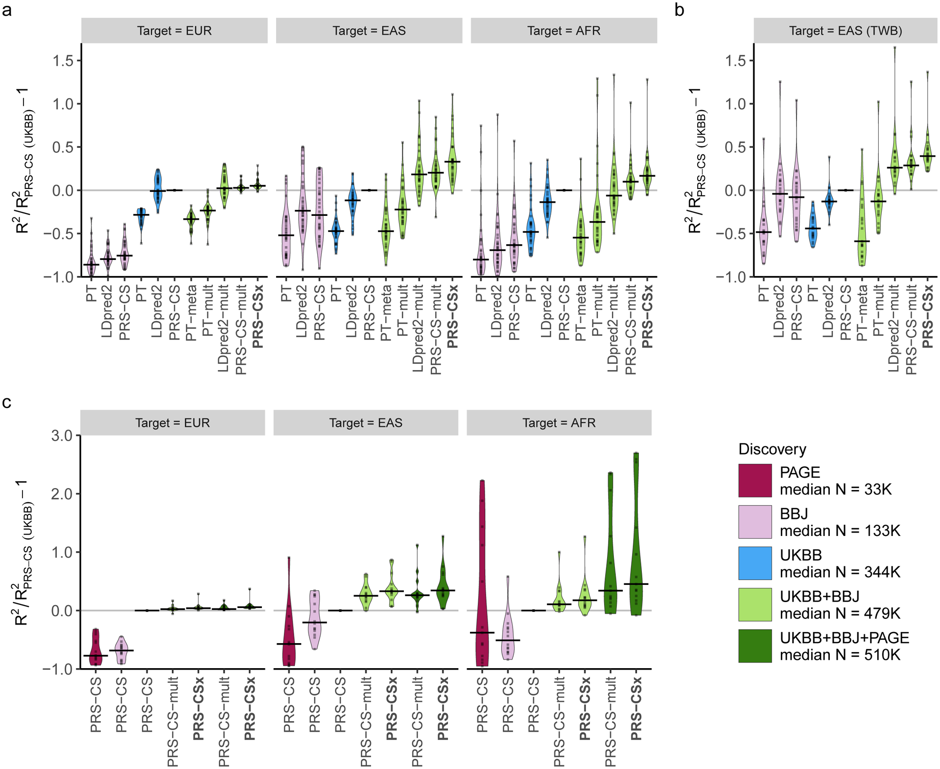
Relative prediction performance for single-discovery and multi-discovery PRS construction methods using discovery GWAS summary statistics a, from UKBB and BBJ, across 33 traits, in different UKBB target populations (EUR, EAS and AFR); b, from UKBB and BBJ, across 21 traits, in the Taiwan Biobank (TWB); c, from UKBB, BBJ and PAGE, across 14 traits, in different UKBB target populations (EUR, EAS and AFR). Each data point shows the relative increase of prediction performance, defined as R²/R²_{PRS-CS (UKBB)} - 1, in which R²_{PRS-CS (UKBB)} is the R² of the trait in the same target population using PRS-CS trained on the UKBB GWAS summary statistics. In UKBB target populations (panels a and c), R² was averaged across 100 random splits of the target samples into validation and testing datasets. The crossbar indicates the median of the relative increase of predictive performance across the traits examined. “median N” indicates the median sample size across the respective discovery GWAS. The trait MCHC was not included in the AFR panel because its R² from PRS-CS (UKBB) was almost 0, which inflated relative increase of prediction performance for other methods.

When predicting into the EUR population, PRS-CSx provided a consistent but marginal improvement over LDpred2 (median relative increase in R²: 4.7%) and PRS-CS (median relative increase in R²: 5.2%), likely due to the limited power of the BBJ GWAS relative to the UKBB GWAS in EUR prediction. The benefit of the coupled prior in this case was also limited, as reflected by a small improvement of PRS-CSx relative to PRS-CS-mult (median relative increase in R²: 2.2%; Fig. 3a, left panel; Supplementary Table 11), which was consistent with the observations in simulations. When the target population was EAS, however, PRS-CSx substantially increased the prediction accuracy relative to single-discovery methods: the median relative improvements in R² were 52.3% and 32.9% when compared with LDpred2 and PRS-CS trained on UKBB GWAS, and 69.8% and 74.4% when compared with LDpred2 and PRS-CS trained on BBJ GWAS, suggesting that PRS-CSx can leverage large-scale EUR GWAS to improve the prediction in non-EUR populations. PRS-CSx also had a median improvement of 10.5% (two-sided Wilcoxon signed-rank test P_wilcoxon=3.90E-4) and 8.3% (P_wilcoxon=2.84E-6) relative to LDpred2-mult and PRS-CS-mult, respectively, demonstrating the benefits of jointly modeling summary statistics from multiple populations in trans-ancestry prediction (Fig. 3a, middle panel; Supplementary Table 11). When the target population did not match any of the discovery samples, PRS-CSx was still able to increase the prediction accuracy. For example, when predicting into the AFR population, the median improvements of PRS-CSx relative to LDpred2 and PRS-CS trained on UKBB GWAS were 45.1% and 16.9%, respectively, and the median improvements relative to LDpred2-mult and PRS-CS-mult were 22.2% (P_wilcoxon=2.38E-5) and 7.1% (P_wilcoxon=2.99E-5), respectively (Fig. 3a, right panel; Supplementary Table 11).

We next sought to replicate the relative performance of different PRS construction methods in the Taiwan Biobank (TWB)³², which is a community-based prospective cohort study of the Taiwanese population. Among the 33 quantitative traits we examined in UKBB and BBJ, 21 traits were also available in TWB. All PRS were trained on the UKBB and/or BBJ GWAS, validated in the UKBB EAS samples (where hyper-parameters were learnt; Supplementary Table 12), and evaluated in the TWB sample comprising 10,149 unrelated individuals, adjusting for age, sex and top 20 PCs of the genotypes. Figure 3b shows that single-discovery methods trained on UKBB and BBJ GWAS had similar performance in the TWB sample, even though UKBB GWAS were much larger (Fig. 3b; Supplementary Table 13). Bayesian multi-discovery methods showed substantial improvement in prediction accuracy compared with single-discovery methods. PRS-CSx provided a median improvement of 39.5% relative to PRS-CS (the best single-discovery method) and 8.2% relative to PRS-CS-mult (the second best multi-discovery method), suggesting the robustness of PRS-CSx when model parameters learnt in validation datasets were applied to external independent testing datasets. Overall, results in the TWB closely reproduced the patterns observed in the UKBB EAS samples (Fig. 3a, middle panel).

We further investigated whether adding African American samples to the discovery dataset can improve the prediction in the AFR population. Among the 33 traits we examined, 14 traits were also available in PAGE³¹ (N=11,178–49,796), a genetic epidemiology study comprising largely African American and Hispanic/Latino samples (Supplementary Table 10). All UKBB-PAGE and BBJ-PAGE genetic-effect correlations were moderate to high (range 0.44–1.00; Supplementary Table 10). Although the discovery and target samples had largely matched ancestry, applying PRS-CS (or other single-discovery methods) to PAGE summary statistics alone produced low prediction accuracy in the AFR population with only a few exceptions, due to the small sample size of the PAGE study (Fig. 3c; Supplementary Table 14). However, integrating UKBB, BBJ and PAGE summary statistics using PRS-CSx (Supplementary Table 15) dramatically outperformed single-discovery methods, and the median relative improvement in R² was 28.1% when compared with PRS-CSx trained on UKBB and BBJ GWAS only, suggesting that PRS-CSx benefits from including samples that have matched ancestry with the target population in the discovery dataset, even if the non-European GWAS included are considerably smaller than European studies (Fig. 3c; Supplementary Tables 14). We note, however, that the overall prediction accuracy in the AFR population remained low relative to the predictions in EUR and EAS individuals, reflecting highly imbalanced sample sizes in the training GWAS across populations (Extended Data Fig. 8). We additionally assessed the convergence of the model fitting algorithm used in PRS-CSx, and confirmed that the Gibbs sampler achieved reasonable convergence and mixing³⁸ (Supplementary Note; Extended Data Fig. 9).

Schizophrenia risk prediction

Lastly, we evaluated the predictive performance of different polygenic prediction methods for dichotomous traits. We used schizophrenia as an example, for which large-scale EUR and EAS GWAS along with multiple individual-level cohorts are available (Supplementary Table 16). Specifically, we used GWAS summary statistics derived from the Psychiatric Genomics Consortium (PGC) wave 2 EUR samples (33,640 cases and 43,456 controls)³⁴ and 10 PGC EAS cohorts¹⁵ (7,856 cases and 11,562 controls) as the discovery dataset. For the additional 7 EAS cohorts which we had access to individual-level data, we set aside one cohort (KOR1; 687 cases and 492 controls) as the validation dataset (for hyper-parameter tuning), and applied a leave-one-out approach to the remaining 6 cohorts. More specifically, we in turn used one of the 6 cohorts as the testing dataset, and meta-analyzed the remaining 5 cohorts with the 10 PGC EAS cohorts using an inverse-variance-weighted meta-analysis to generate the discovery GWAS summary statistics for the EAS population. The prediction accuracy of different PRS construction methods was then evaluated in the left-out (testing) cohort, adjusting for sex and top 20 PCs.

Consistent with previous observations, PRS trained on EAS GWAS were more predictive in EAS cohorts than those trained on PGC EUR summary statistics¹⁵, despite the larger sample size for the EUR GWAS (Fig. 4a; Supplementary Table 17). Among single-discovery methods examined, LDpred2 and PRS-CS performed substantially better than PT, highlighting the importance of modeling LD patterns for highly polygenic traits. By integrating EUR and EAS summary statistics, Bayesian multi-discovery methods dramatically increased the prediction accuracy relative to single-discovery methods. Compared with LDpred2, the best-performing single-discovery method in this analysis, PRS-CSx increased the median R² on the liability scale (assuming 1% of disease prevalence) from 0.043 (LDpred2 trained on EAS GWAS) and 0.031 (LDpred2 trained on EUR GWAS) to 0.063, a relative increase of 45.4% and 104.9%, respectively. PRS-CSx also approximately doubled the prediction accuracy of PT-meta and PT-mult, with a relative increase of 135.9% (from 0.027 to 0.063) and 95.3% (from 0.032 to 0.063) in the median liability R², respectively. In addition, PRS-CSx provided consistent, although relatively small, improvement over LDpred2-mult (relative increase in median R²: 8.7%) and PRS-CS-mult (relative increase in median R²: 5.9%), suggesting that in practice PRS-CSx can increase predictive power over Bayesian “mult” methods even for highly polygenic architecture (Fig. 4a; Supplementary Table 17), a scenario where the benefit of the coupled prior was reduced in simulations (Extended Data Fig. 1; Supplementary Table 2). Other performance metrics, including Nagelkerke’s R², odds ratio (OR) per standard deviation change of PRS, and OR comparing top 10% with bottom 10% of the PRS distribution, showed a consistent pattern (Supplementary Table 17). Finally, PRS-CSx can more accurately identify individuals at high/low schizophrenia risk than alternative methods, showing a 2.9, 3.5 and 4.2-fold increase in the proportion of schizophrenia cases across the 6 testing cohorts when contrasting the top 10%, 5% or 2% of the PRS distribution with the bottom 10%, 5% or 2%, respectively (Fig. 4b; Supplementary Table 18).

Figure 4: Prediction accuracy of schizophrenia risk in EAS cohorts.

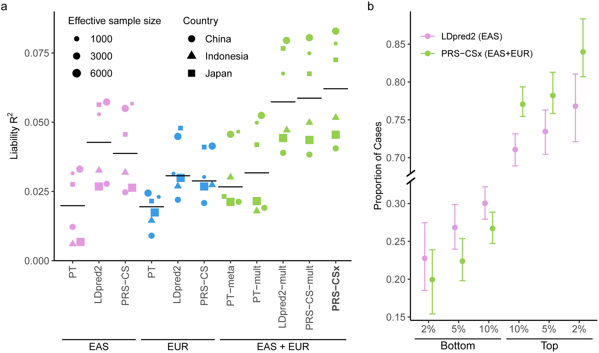
a, Prediction accuracy, measured as variance explained (R²) on the liability scale, of single-discovery (trained on EAS or EUR GWAS) and multi-discovery polygenic prediction methods (trained on both EAS and EUR GWAS: EAS+EUR) across 6 EAS schizophrenia cohorts. Each dot represents one testing cohort, with the size of the dot being proportional to its effective sample size, calculated as 4/(1/Ncase+1/Ncontrol), and the shape of the dot representing the country where the sample was collected. Crossbar indicates the median R² on the liability scale. b, The center of the error bar shows the proportion of schizophrenia cases of the bottom 2%, 5%, 10% and top 2%, 5%, 10% of the PRS distribution, constructed by LDpred2 trained on EAS GWAS (the best-performing single-discovery method) and PRS-CSx (the best-performing multi-discovery method), across 6 EAS schizophrenia cohorts (9,416 cases, 8,708 controls). Error bar indicates 95% confidence intervals.

DISCUSSION

We have presented PRS-CSx, a Bayesian polygenic prediction method that integrates GWAS summary statistics from multiple populations to improve the prediction accuracy of PRS in ancestrally diverse samples. PRS-CSx leverages the correlation of genetic effects and LD diversity across populations to more accurately localize association signals and increase the effective sample size of the discovery dataset, while accounting for population-specific allele frequency and LD patterns. We have shown, via simulation studies, that PRS-CSx robustly improves cross-population prediction over existing methods across traits with varying genetic architectures, genetic overlaps between populations, and discovery GWAS sample sizes. Using quantitative traits from multiple biobanks as well as schizophrenia cohort studies of European and East Asian ancestries, we have further demonstrated the PRS-CSx can leverage large-scale European GWAS to boost the accuracy of polygenic prediction in non-European populations, for which ancestry-matched discovery GWAS may be orders of magnitude smaller in sample size.

PRS-CSx is expected to provide larger power gains when the GWAS in the target population has lower statistical power, while well-powered GWAS from other populations are available. This often happens when predicting into a non-EUR population, where ancestry-matched GWAS have limited sample sizes but large-scale EUR GWAS already exist. By integrating EUR and non-EUR GWAS, PRS-CSx can significantly improve the prediction accuracy in non-EUR populations, which alleviates the imminent challenge of polygenic prediction in under-represented populations. In contrast, PRS-CSx may provide limited increase in prediction accuracy when a well-powered GWAS in the target population already exists and GWAS from other populations have smaller sample sizes and lower statistical power. In practice, this happens almost exclusively for predictions in the EUR population. We note that while PRS-CSx increased the prediction in non-European populations for the majority of the traits examined in this study, the amount of improvement in prediction accuracy over alternative methods varied across traits. Future research is needed to dissect the effects of potential factors on the accuracy of cross-ancestry polygenic prediction and to better understand the behavior of different prediction algorithms for individual traits.

PRS-CSx is designed to flexibly model GWAS summary statistics from multiple populations where SNP effect sizes and/or LD patterns differ. For two or more GWAS conducted in independent samples from the same population where effect sizes and LD patterns are expected to be highly concordant, a fixed-effect meta-analysis is probably the optimal approach to combine the GWAS and maximize statistical power. However, we do not recommend meta-analyzing summary statistics across populations and applying single-discovery methods (e.g., LDpred2 or PRS-CS) to the meta-GWAS for two reasons: (1) The LD pattern of a cross-ancestry meta-analyzed GWAS is a mixture of population-specific LD, which is difficult to appropriately model. Rather, accurately modeling LD patterns is often crucial to the performance of Bayesian polygenic prediction methods. (2) The predictive performance of these “meta” methods heavily depends on whether the assumption of the fixed-effect meta-analysis (i.e., consistent SNP effects across populations) is accurate. These methods are thus less adaptive to a wide range of cross-population genetic architectures compared with PRS-CSx or the “mult” methods. That said, many existing studies have only released summary statistics from cross-population meta-analysis, in which case applying single-discovery methods to the meta-GWAS remains useful approaches in practice. We believe that releasing ancestry-specific summary statistics from multi-ancestry genomic studies is critical for understanding comparative genetic architectures between populations, and for flexible and accurate cross-population polygenic modeling and prediction.

The use of PRS-CSx, as well as the “mult” methods examined in this work, requires a validation dataset to tune hyper-parameters and learn the optimal linear combination of population-specific PRS, and an independent testing dataset where the final PRS can be generated and evaluated. As non-European genomic resources remain limited, independent validation and testing datasets are often difficult to identify, and a single target cohort may be too small to be split into validation and testing sets. To facilitate the use of PRS-CSx, we have released posterior SNP effects and linear combination weights for all the traits and target populations examined in this study. In addition, in certain applications, it may be preferable to calculate PRS for all samples within the target cohort rather than stratifying them into different ancestry groups. For example, returning genomic predictions to patients with recently admixed ancestries in clinical settings would be difficult as ancestries are not distinct entities, and genetic ancestry assignments may be inconsistent with self-reported race/ethnicity, illuminating the complexity of communicating population-stratified PRS results to patients. In these scenarios, PRS-CSx provides an “auto” version which automatically learns the global shrinkage parameter from the discovery summary statistics, and a “meta” option which integrates population-specific posterior SNP effects using an inverse-variance-weighted meta-analysis within the Gibbs sampler. Combining the “auto” and “meta” algorithms thus generates a trans-ancestry PRS that can be applied to all samples in the target cohort without the need for a validation dataset³⁹. We note that, although simpler to implement, the “meta” option is expected to be less accurate compared with the linear combination approach that optimizes PRS estimation separately in each target population.

While PRS-CSx can take an arbitrary number of GWAS summary statistics as input, an ancestry-matched LD reference panel is required for each discovery sample, which may be challenging to build for GWAS conducted in admixed populations or in samples with large genomic diversity⁴⁰. Although we have shown that PRS-CSx is robust to imperfectly matched LD reference panels, future work is needed to better model summary statistics from recently admixed populations^41,42.

Lastly, we note that although PRS-CSx can improve cross-population polygenic prediction, the gap in the prediction accuracy between European and non-European populations remains considerable. Indeed, sophisticated statistical and computational methods alone will not be able to overcome the current Eurocentric biases in GWAS. Broadening the sample diversity in genomic research to fully characterize the genetic architecture and understand the genetic and non-genetic contributions to human complex traits and diseases across global populations is crucial to further improve the prediction accuracy of PRS in diverse populations.

METHODS

PRS-CSx.

PRS-CSx is an extension of PRS-CS¹⁹, which enables the integration of GWAS summary statistics from multiple populations to improve cross-population polygenic prediction. Consider the following Bayesian high-dimensional linear regression model for K populations:

$$y_k=X_k{\beta }_k+{ϵ}_k,\hspace{1em}{ϵ}_k~\text{MVN}\left(0,{\sigma }_k^{2}I\right),\hspace{1em}\pi \left({\sigma }_k^2\right)\propto {\sigma }_k^{-2},\hspace{1em}k=1,2,\cdots ,K,$$

where, for each population k, y_k is a vector of standardized phenotypes (zero mean and unit variance) from N_k individuals, X_k is an N_k × M_k matrix of standardized genotypes (each column has zero mean and unit variance), β_k is a vector of SNP effect sizes, ϵ_k is a vector of normally distributed non-genetic effects with variance ${\sigma }_k^2$, for which we assign a non-informative scale-invariant Jeffreys prior, and I is an identify matrix. We use j = 1, 2, ⋯ , M to index the M unique SNPs across populations. For SNP j in population k, we place a continuous shrinkage prior on its effect size β_jk, which can be represented as global-local scale mixtures of normals:

$${\beta }_{jk}~\text{N}\left(0,\frac{{\sigma }_k^2}{N_k}{\psi }_j\right),\hspace{1em}{\psi }_j~\text{Gamma}\left(a,{\delta }_j\right),\hspace{1em}{\delta }_j~\text{Gamma}\left(b,\varphi \right),$$

where ϕ is a global shrinkage parameter shared across all SNPs that models the overall sparseness of the genetic architecture, and Ψ_j is a local, SNP-specific shrinkage parameter that is adaptive to marginal GWAS associations. By assigning a gamma-gamma hierarchical prior on Ψ_j (specifically, the Strawderman-Berger prior with a = 1 and b = 1/2 in this work), the marginal prior density of β_jk has sizable amount of mass near zero to impose strong shrinkage on small noisy signals, and in the meantime, heavy Cauchy-like tails to avoid over-shrinkage of truly non-zero effects.

We note that when SNP j is available in multiple GWAS summary statistics, the continuous shrinkage prior is shared across populations (i.e., both ϕ and Ψ_j do not depend on k), enabling information sharing between summary statistics while allowing for varying SNP effect sizes across populations to retain modeling flexibility. More specifically, given the variance parameters ${\sigma }_k^2$, ϕ and Ψ_j, and the marginal least squares estimates of the SNP effect sizes in population k, ${\widehat{\beta }}_k=X_k^T{y}_k/N_k$, the posterior mean of β_k is $\text{E}\left[{\beta }_k|{\widehat{\beta }}_k\right]={(D_k+{\Psi }^{-1})}^{-1}{\widehat{\beta }}_k$, where $D_k=X_k^T{X}_k/N_k$ is the LD matrix for population k, and Ψ = diag{Ψ₁, Ψ₂, ⋯ ,Ψ_M} is a diagonal matrix (Supplementary Note). It can be seen that Ψ does not depend on k and thus the amount of shrinkage applied to each SNP is shared across populations. Meanwhile, population-specific LD patterns are explicitly modelled via the LD matrix D_k.

Given the summary statistics and ancestry-matched LD reference panel for each discovery sample, the PRS-CSx model can be fitted using a Gibbs sampler with block update of posterior SNP effect sizes, without the need to access individual-level data (Supplementary Note). Monomorphic or rare variants not present in the GWAS summary statistics or population-specific LD reference panel of population A are not included in the construction of PRS for population A. If a SNP is present in population A but is monomorphic or rare in other populations, its effect size is not coupled across populations in posterior inference but the SNP is included in the PRS of population A such that population-specific associations can be captured (Fig. 1). In the extreme, unlikely scenario, where there is no overlapping SNP between input GWAS summary statistics, PRS-CSx reduces to applying PRS-CS separately to each discovery GWAS. PRS-CSx inherits many features from PRS-CS, including robustness to varying genetic architectures, multivariate modeling of population-specific LD patterns, and computational efficiency. In this work, we used pre-calculated 1KG Phase 3 LD reference panels⁴³ for EUR, EAS, AFR and AMR populations, which were constructed for HapMap3 variants with MAF >1%. We recommend using 1,000*K Markov Chain Monte Carlo (MCMC) iterations with the first 500*K steps as burin-in in Gibbs sampling, where K is the number of discovery populations, reflecting the growing number of unknown parameters with the number of discovery GWAS jointly modelled. For a fixed global shrinkage parameter ϕ, PRS-CSx returns posterior SNP effect size estimates for each discovery population, which can be used to calculate K population-specific PRS in the target sample. For each ϕ value, we fitted a linear (or logistic) regression of the z-scored PRS (one for each discovery population) in the validation dataset:

$$y~w_{\varphi ,1}PR{S}_{\varphi ,1}+w_{\varphi ,2}PR{S}_{\varphi ,2}+\cdots +w_{\varphi ,K}PR{S}_{\varphi ,K},$$

where y is the trait of interest, PRS_ϕ,k is the standardized PRS for population k, and w_ϕ,k is the regression coefficient. We screened four different ϕ values, 10⁻⁶, 10⁻⁴, 10⁻² and 1.0, in this work. The ϕ value and the corresponding regression coefficients for the linear combination of PRS that maximized the R² in the validation dataset were used in the testing dataset to calculate the final PRS:

$$PRS={\widehat{w}}_{\widehat{\varphi },1}PR{S}_{\widehat{\varphi },1}+{\widehat{w}}_{\widehat{\varphi },2}PR{S}_{\widehat{\varphi },2}+\cdots +{\widehat{w}}_{\widehat{\varphi },K}PR{S}_{\widehat{\varphi },K}.$$

Alternative PRS construction methods

PT:

LD-informed pruning and p-value thresholding (PT)³⁵ selects clumped SNPs of a certain statistical significance to be included in the PRS calculation. We performed PT using PRSice-2⁴⁴ with the default parameter settings: the clumping was performed with a radius of 250kb and an r² threshold of 0.1. We used 1KG super-population samples (EUR, EAS, AFR or AMR) whose ancestry matched the discovery sample as the LD reference panel for clumping. The p-value threshold among 10⁻⁸, 10⁻⁷, 10⁻⁶, 10⁻⁵, 3×10⁻⁵, 10⁻⁴, 3×10⁻⁴, 0.001, 0.003, 0.01, 0.03, 0.1, 0.3 and 1.0 that maximized the R² in the validation dataset was selected, and used in the independent testing dataset to calculate the final PRS and its performance metrics.

LDpred2:

LDpred2²⁰, an improved version of the LDpred algorithm²¹, is a Bayesian polygenic prediction method that adjusts marginal SNP effect size estimates from GWAS summary statistics to calculate the PRS. LDpred2 assigns a point-normal prior to SNP effect sizes, where the proportion of causal variants is a tunable parameter, and infers posterior effects using a Gibbs sampler. We constrained the computation to HapMap3 variants with MAF >1%, and used 1KG super-population samples (EUR, EAS, AFR or AMR) whose ancestry matched the discovery sample as the LD reference panel. We ran LDpred2-grid using the genome-wide option with the full LD matrix, and tested the proportion of causal variants from a sequence of 17 values equally spaced from 10⁻⁴ to 1.0 on the log scale. The proportion that maximized the R² in the validation dataset was selected, and used in the independent testing dataset to calculate the final PRS and its performance metrics.

PRS-CS:

PRS-CS¹⁹ is a Bayesian polygenic prediction method that infers posterior SNP effect sizes from summary statistics using a continuous shrinkage prior, which is robust to varying genetic architectures, accurate in LD modeling and computationally efficient. PRS-CS has one hyper-parameter, the global shrinkage parameter, which models the overall sparseness of the genetic architecture. We used default parameter settings and the pre-calculated 1KG LD reference panel (EUR, EAS, AFR or AMR) that matched the ancestry of the discovery sample, which was constructed for HapMap3 variants with MAF >1%. The global shrinkage parameter among 10⁻⁶, 10⁻⁴, 10⁻² and 1.0 that maximized the R² in the validation dataset was selected, and used in the independent testing dataset to calculate the final PRS and its performance metrics.

PT-meta:

PT-meta applies PT to the meta-GWAS that combines all discovery summary statistics through an inverse-variance-weighted fixed-effect meta-analysis. We used the same clumping parameters and screened the same list of p-value thresholds as the PT method. The 1KG LD reference panel (EUR, EAS, AFR or AMR) that had matched ancestry with each of the discovery samples was in turn used for clumping, producing multiple sets of clumped variants. The best combination of the LD reference panel and the p-value threshold that maximized the R² in the validation dataset was selected, and used in the independent testing dataset to calculate the final PRS and its performance metrics.

PT-mult, LDpred2-mult and PRS-CS-mult:

PT-mult²⁶, LDpred2-mult and PRS-CS-mult apply PT, LDpred2 and PRS-CS to each discovery summary statistics separately. The most predictive PRS derived from each discovery sample were then used to fit a linear regression in the validation dataset:

$$y~w_{1}PR{S}_1+w_{2}PR{S}_2+\cdots +w_{K}PR{S}_K,$$

where PRS_k is the standardized PRS for population k, and w_k is the corresponding regression coefficient. The optimal hyper-parameter for each discovery sample and the estimated regression coefficients for the linear combination of standardized PRS were used in the independent testing dataset to calculate the final PRS and its performance metrics. We screened the same grid of hyper-parameters for each method (i.e., the p-value threshold for PT; the proportion of causal variants for LDpred2; and the global shrinkage parameter for PRS-CS). The 1KG super-population samples (EUR, EAS, AFR or AMR) whose ancestry matched the discovery sample were used as the LD reference panel.

Simulations.

Genotypes:

We simulated individual-level genotypes of EUR, EAS and AFR populations using HAPGEN2³⁷ with ancestry-matched 1KG Phase 3³⁶ super-population samples as the reference panel. We grouped CEU, IBS, FIN, GBR and TSI into the EUR super-population, CDX, CHB, CHS, JPT and KHV into the EAS super-population, and ACB, ASW, LWK, MKK and YRI into the AFR super-population. To calculate the genetic map (cM) and recombination rate (cM/Mb) for each super-population, we downloaded the maps and rates for their constituent subpopulations (Data availability), linearly interpolated the genetic map and recombination rate at each position (Code availability), and averaged the genetic maps and recombination rates across the subpopulations within each super-population. We simulated 320K EUR samples, 100K EAS samples and 100K AFR samples, and confirmed that the allele frequencies and LD patterns of the simulated genotypes were highly similar to those of the 1KG reference panels. We note, however, that while highly scalable, genotypes simulated by HAPGEN2 may not fully capture the complex population structure within and across ancestry groups. We saved 20K samples for each of the three populations as the target dataset, which was evenly split into validation and testing datasets. The remaining samples served as the discovery dataset, which was used to produce GWAS of varying sample sizes. We constrained the simulations to 1,296,253 HapMap3 variants with MAF >1% in at least one of the EUR, EAS and AFR populations, and removed triallelic and strand ambiguous variants.

Phenotypes:

In our primary simulation, we randomly sampled 1% of the HapMap3 variants as causal variants. We assumed that causal variants are shared across the three populations and simulated their per-allele effect sizes using a multivariate normal distribution with the correlation between populations set to 0.7. For each population, we used a normally distributed random variable to model the non-genetic component such that the heritability was fixed at 50%. The phenotype was then generated in each population using y = Xβ + ϵ, where X was the genotype matrix, β was the simulated per-allele effect size vector in which causal variants had non-zero effects and the rest of the variants had zero effect sizes, and ϵ was the simulated non-genetic component. The simulation was repeated 20 times. GWAS was performed on 100K EUR, 20K EAS and 20K AFR discovery samples, respectively, using PLINK 1.9⁴⁵.

We conducted a series of secondary simulations to assess the robustness of PRS-CSx in a wide range of settings: (i) varying polygenicity of the genetic architecture (0.1% vs. 1% vs. 10% of causal variants); (ii) varying cross-population genetic correlations (r_g=0.4 vs. r_g=0.7 vs. r_g=1.0); (iii) varying sample sizes of the discovery GWAS (50K EUR + 10K non-EUR; 100K EUR + 20K non-EUR; 200K EUR + 40K non-EUR; 300K EUR + 60K non-EUR); (iv) varying ratios of the EUR vs. non-EUR GWAS sample sizes (120K EUR + 0K non-EUR; 100K EUR vs. 20K non-EUR; 80K EUR + 40K non-EUR; 60K EUR + 60K non-EUR); (v) varying SNP heritability of the simulated trait in different populations (h²=0.5 in EUR + h²=0.5 in non-EUR; h²=0.5 in EUR + h²=0.25 in non-EUR; h²=0.25 in EUR + h²=0.5 in non-EUR); (vi) varying proportions of shared causal variants across populations (100% vs. 70% vs. 40%); (vii) allele frequency and LD dependent genetic architecture: instead of sampling per-allele SNP effect sizes from a multivariate normal distribution with homogeneous variance across the genome, we assumed that the variance of SNP j in population k is proportional to ${[2f_{jk}\left(1-f_{jk}\right)]}^{\alpha }{\ell }_{jk}^{\alpha }$, where f_jk and ℓ_jk are the MAF and LD score of SNP j in population k, respectively. When α < 0 , variants with lower MAF and variants located in lower LD regions tend to have larger effects on the trait^46–48. We used α = −0.25 in this set of simulations, which has been empirically estimated to reflect the relationship between effect size and allele frequency⁴⁶. This α value produced approximately a 4-fold difference in the variance of per-allele effect size for both high-frequency vs. low-frequency variants and high-LD vs. low-LD variants included in the simulations; (ix) varying hyper-parameters in the continuous shrinkage prior (a=0.5, b=0.5 vs. a=1.0, b=0.5 vs. a=1.5, b=0.5 vs. a=1.0, b=1.0).

UKBB, BBJ, PAGE and TWB analysis.

Discovery data:

We downloaded GWAS summary statistics from UKBB²⁸, BBJ²⁹ and PAGE³¹ (Data availability). We selected 33 quantitative traits that were available in both UKBB and BBJ, among which 14 were also available in PAGE (Supplementary Table 10). We used 1KG EUR and EAS samples as the LD reference panel for UKBB and BBJ summary statistics, respectively, when constructing PRS. The PAGE study was largely comprised African American and Hispanic/Latino samples, for which we used the 1KG AMR reference panel as an approximation in the PRS analyses. UKBB target data: All UKBB target samples are unrelated UKBB individuals that are non-overlapping and unrelated with the UKBB GWAS sample. To perform population assignment on the UKBB samples, we selected variants that are available in both 1KG and the UKBB genotyped dataset, and removed variants meeting one of the following criteria in 1KG: (i) strand ambiguous; (ii) located on sex chromosomes or in long-range LD regions (chr6: 25–35Mb; chr8: 7–13Mb); (iii) call rate <0.98; and (iv) MAF <0.05. We performed LD pruning on the remaining variants in 1KG using PLINK⁴⁵ (--indep-pairwise 100 50 0.2), yielding 149,501 largely independent, high-quality common variants. We then conducted principal component analysis using these LD-pruned SNPs in 1KG samples, and projected SNP loadings onto UKBB samples with the scale appropriately adjusted. Using 1KG as the reference, we trained a random forest model to predict the 5 super-population labels (AFR, AMR, EAS, EUR, SAS) using the top 6 PCs, and applied the trained random forest classifier to UKBB samples to predict the genetic ancestry of each UKBB participant. We retained UKBB samples that can be assigned to one of the super-populations with a predicted probability >90%. For each population in UKBB, we selected a set of unrelated individuals and performed sample-level quality control (QC) by removing individuals meeting one of the following criteria: (i) mismatch between self-reported and genetically inferred sex; (ii) missingness or heterozygosity outliers; and (iii) sex chromosome aneuploidy. For the validation and testing of PRS in the EUR population, we used non-British EUR samples that are unrelated to the White British samples included in Neale Lab UKBB GWAS. Lastly, we converted imputed dosage data into hard coded genotypes using PLINK 2.0 with default parameters (i.e., dosage was rounded to the nearest hardcall when the distance was no great than 0.1; otherwise a missing hardcall was saved), and performed variant-level QC within each target population by removing variants meeting one of the following criteria: (i) call rate <0.98; (ii) MAF <0.01; (iii) Hardy-Weinberg equilibrium test p-value <10⁻¹⁰; and (iv) imputation INFO score <0.8. The final target dataset included 7,507 AFR, 687 AMR, 2,181 EAS, 14,085 EUR and 8,412 SAS individuals, with 12,886,200, 8,593,932, 6,506,126, 8,211,053 and 8,032,121 variants, respectively. TWB target data: The Taiwan Biobank (TWB)^32,33 is a prospective cohort study of the Taiwanese population. Participants were 30 to 70 years old at recruitment. Among the 33 quantitative traits examined in UKBB, we identified 21 traits that were also available in TWB. We used 14,232 samples genotyped on the TWBv2 custom array and imputed against the 1KG samples, the same dataset used in the PRS analysis of our recent TWB quantitative trait GWAS study³², to evaluate the predictive performance of different polygenic prediction methods. Following the same sample-level and variant-level QC procedures used in the UKBB analysis, the final analytic sample included 10,149 unrelated individuals of EAS ancestry that had complete data across the 21 traits. Detailed information on the sample characteristics and collection of phenotypes can be found in Chen et al.^32,33

Heritability and cross-population genetic correlation.

Heritability of each trait in UKBB, BBJ and PAGE was estimated using LD score regression⁴⁹ with ancestry-matched LD reference panels. We calculated the cross-population genetic correlation between UKBB, BBJ and PAGE using POPCORN¹⁶ with default parameters. POPCORN requires the LD score⁴⁹ and cross-covariance score as the input. We used the pre-computed EUR-EAS scores (available from the POPCORN website), and computed EUR-AFR and EAS-AFR scores on 1KG Phase 3 samples using the ‘compute’ function provided by POPOCORN.

Schizophrenia datasets.

Schizophrenia data used in this study is summarized in Supplementary Table 16. PGC wave 2 schizophrenia GWAS summary statistics³⁴ were used as the European discovery dataset. Except for one cohort (TMIM1), EAS samples used as discovery and target datasets were described in Lam et al.¹⁵ TMIM1 was recruited from multiple university hospitals and local hospitals in Japan. Patients were diagnosed according to the Diagnostic and Statistical Manual of Mental Disorders, 4th Edition (DSM-IV) with consensus from at least two experienced psychiatrists. All patients agreed to participate in the study and provided written informed consent. The study was approved by the Institutional Review Boards of the Tokyo Metropolitan Institute of Medical Science and all affiliated institutions. DNA samples were genotyped on the Illumina Infinium Global Screening Array-24 v1.0 (GSA) BeadChip at the Broad Institute, using standard reagents and HTS workflow procedures. GWAS QC and imputation were performed using Ricopili⁵⁰ with default parameters. When used as a target cohort, SNPs were further filtered by imputation INFO score <0.9 and MAF <0.01.

Ethics.

Collection of the UKBB data was approved by the UKBB’s Research Ethics Committee. UKBB individual-level data used in the present work were obtained under application #32568. BBJ and PAGE: only publicly available GWAS summary statistics, without individual-level information, were used in this study. Collection of the TWB data was approved by the Ethics and Governance Council (EGC) of TWB and the Department of Health and Welfare, Taiwan (Wei-Shu-I-Tzu NO.1010267471). TWB obtained informed consent from all participants for research use of the collected data. The access to and the use of TWB data in the present work was approved by the EGC of TWB (approval number: TWBR10907-05) and the Institutional Review Board of National Health Research Institutes, Taiwan (approval number: EC1090402-E). Schizophrenia GWAS summary statistics of EUR and EAS ancestries are available via the Psychiatric Genomics Consortium, and do not contain any individual-level information. The following institutions provided ethics oversight for schizophrenia East Asian samples used in this work: Samsung Medical Center; Bio-X Institutes of Shanghai Jiao Tong University; Fujita Health University; Tokyo Metropolitan Institute of Medical Science; University Medical Center Utrecht; The University of Western Australia; The University of Indonesia; RIKEN Center for Integrative Medical Sciences; Nagoya University; Osaka University; Niigata University; Chonnam National University Hospital, and Mass General Brigham (Protocols 2014P001342 and 2011P002207). Informed consent and permission to share the data were obtained from all subjects, in compliance with the guidelines specified by the recruiting center’s institutional review board.

Extended Data

Extended Data Fig. 1. Prediction accuracy of different polygenic prediction methods across different genetic architectures.

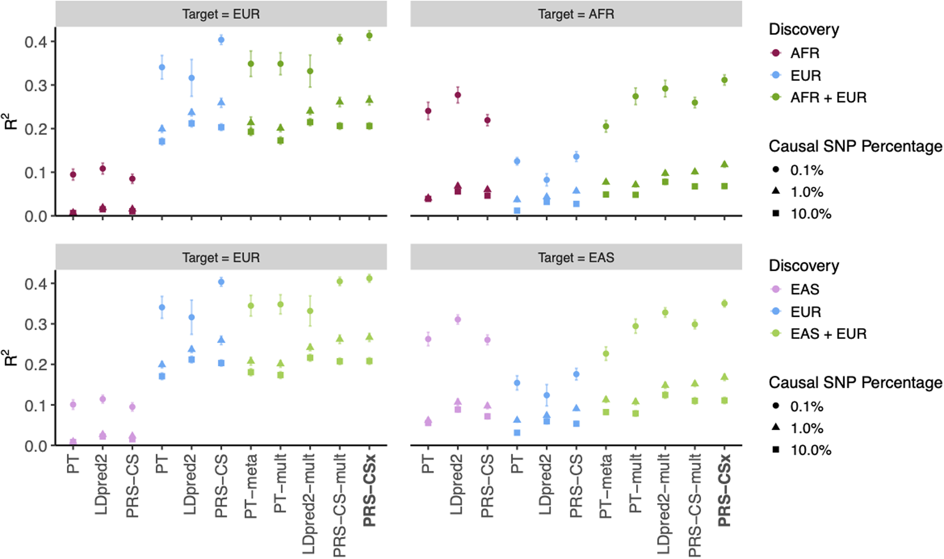
Phenotypes were simulated using 0.1%, 1% or 10% of randomly sampled causal variants (shared across populations), a cross-population genetic correlation of 0.7, and SNP heritability of 50%. PRS were trained using 100K EUR samples and 20K non-EUR (EAS or AFR) samples. Numerical results are reported in Supplementary Table 2.

Extended Data Fig. 2. Prediction accuracy of different polygenic prediction methods across different cross-population genetic correlations.

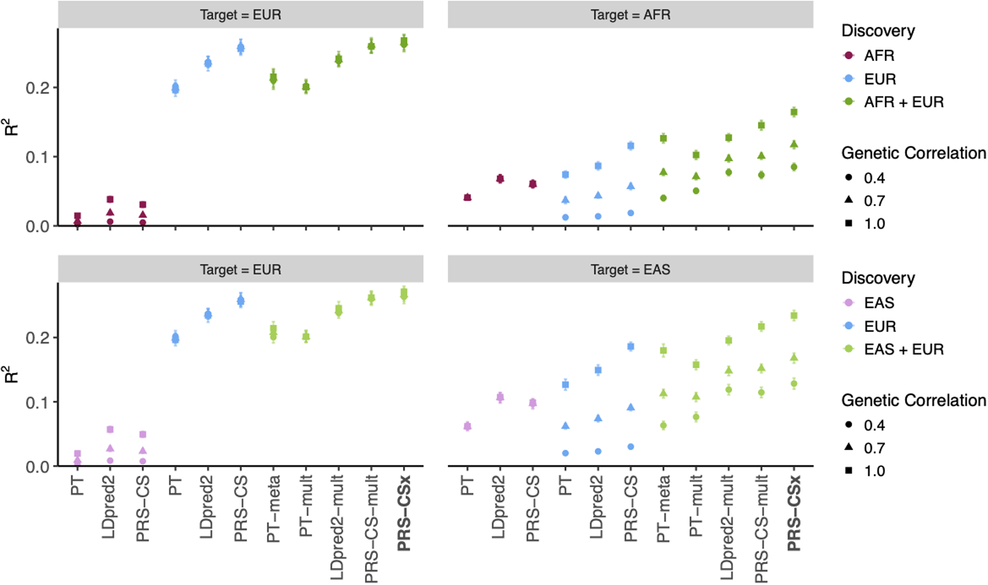
Phenotypes were simulated using 1% of randomly sampled causal variants (shared across populations), a cross-population genetic correlation of 0.4, 0.7 or 1.0, and SNP heritability of 50%. PRS were trained using 100K EUR samples and 20K non-EUR (EAS or AFR) samples. Numerical results are reported in Supplementary Table 3.

Extended Data Fig. 3. Prediction accuracy of different polygenic prediction methods across different discovery GWAS sample sizes.

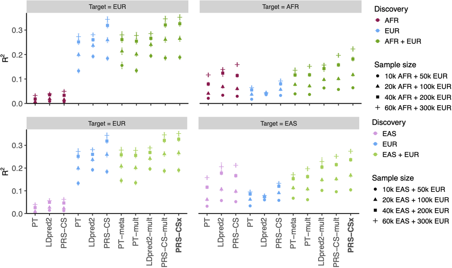
Phenotypes were simulated using 1% of randomly sampled causal variants (shared across populations), a cross-population genetic correlation of 0.7, and SNP heritability of 50%. PRS were trained using 50K EUR and 10K non-EUR (EAS or AFR) samples, 100K EUR and 20K non-EUR samples, 200K EUR and 40K non-EUR samples, or 300K EUR and 60K non-EUR samples. Numerical results are reported in Supplementary Table 4.

Extended Data Fig. 4. Prediction accuracy of different polygenic prediction methods across different ratios of EUR vs. non-EUR GWAS sample sizes.

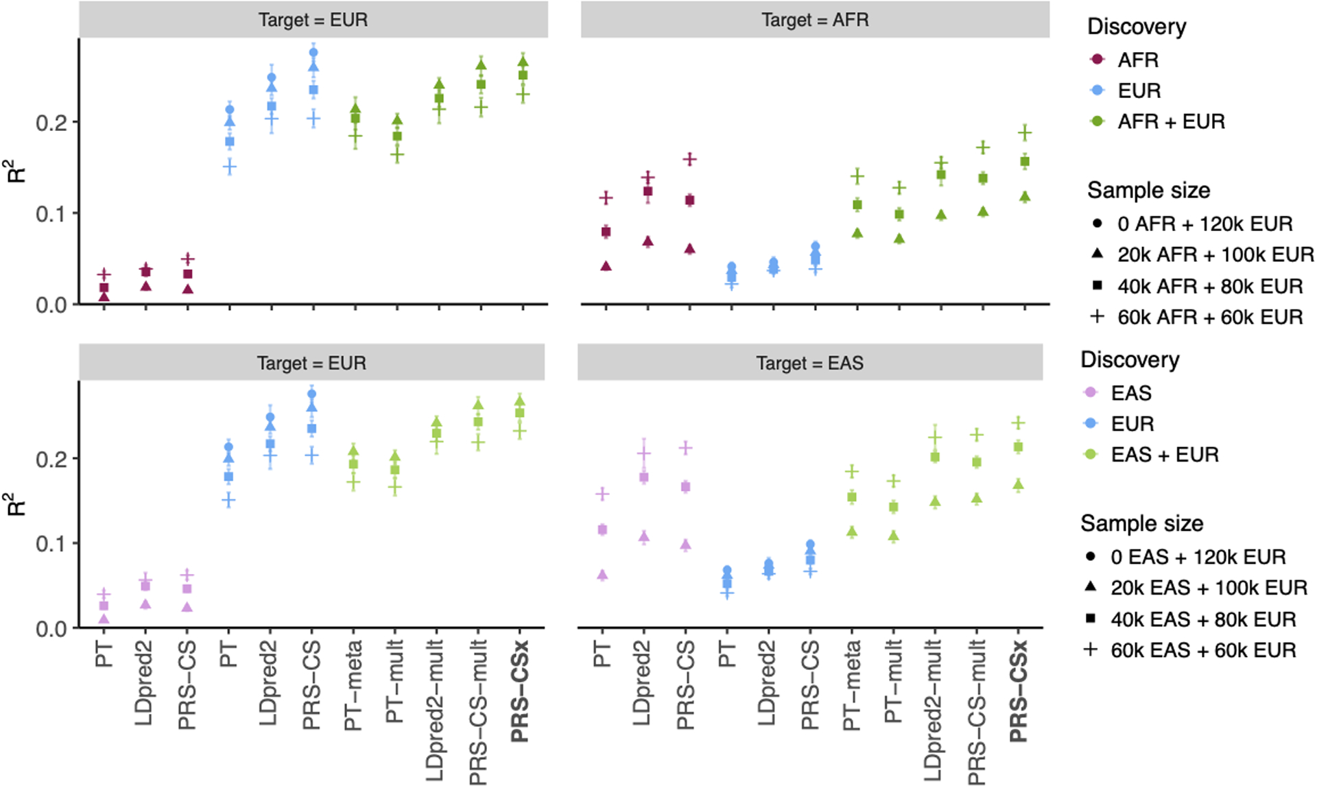
Phenotypes were simulated using 1% of randomly sampled causal variants (shared across populations), a cross-population genetic correlation of 0.7, and SNP heritability of 50%. PRS were trained using 120K EUR samples without non-EUR samples, 100K EUR and 20K non-EUR (EAS or AFR) samples, 80K EUR and 40K non-EUR samples, or 60K EUR and 60K non-EUR samples. Numerical results are reported in Supplementary Table 5.

Extended Data Fig. 5. Prediction accuracy of different polygenic prediction methods across different SNP heritability.

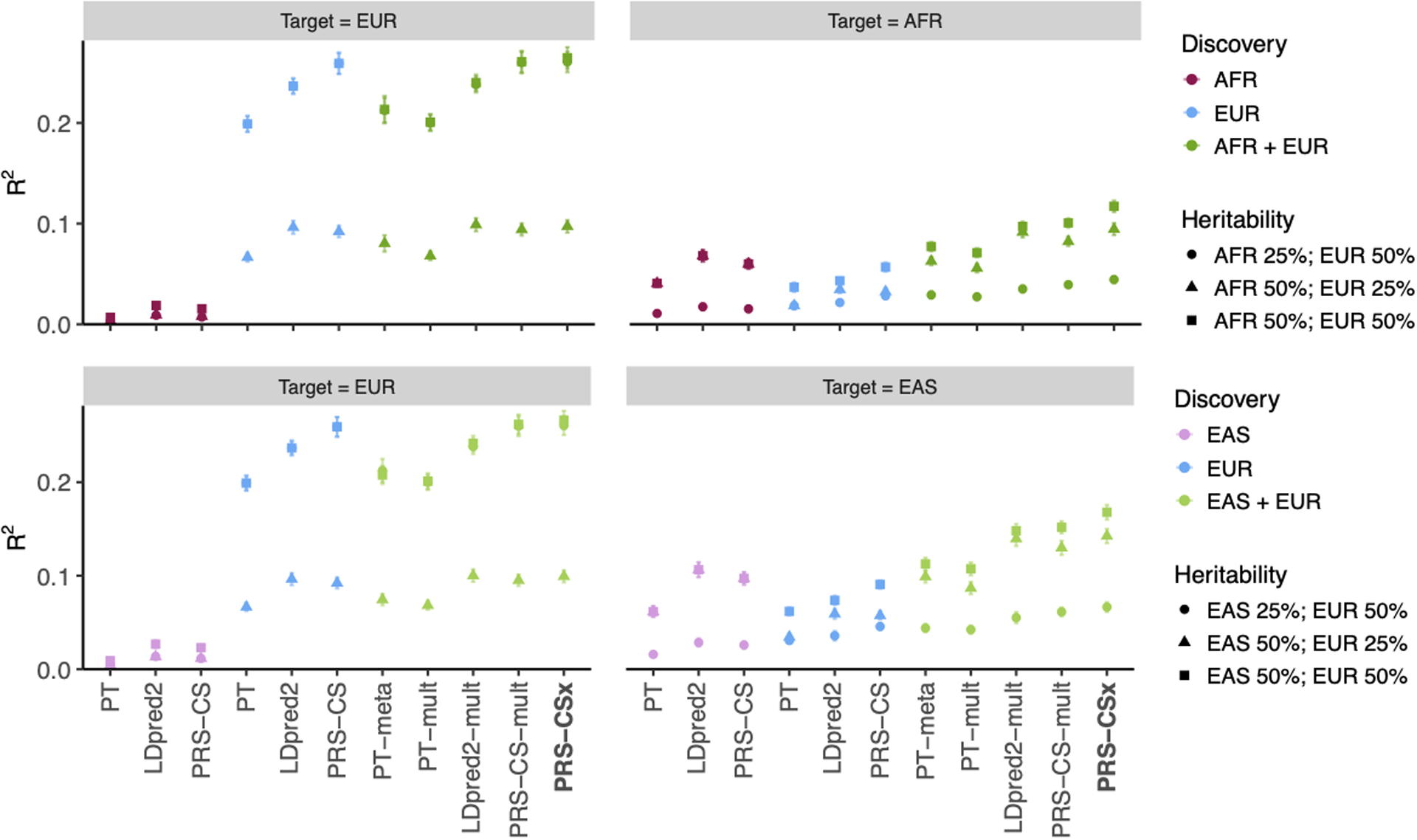
Phenotypes were simulated using 1% of randomly sampled causal variants (shared across populations) and a cross-population genetic correlation of 0.7. SNP heritability was fixed at 50% in each population, 50% in the EUR population and 25% in the non-EUR population, or 25% in the EUR population and 50% in the non-EUR population. PRS were trained using 100K EUR samples and 20K non-EUR (EAS or AFR) samples. Numerical results are reported in Supplementary Table 6.

Extended Data Fig. 6. Prediction accuracy of different polygenic prediction methods across different proportions of shared causal variants between populations.

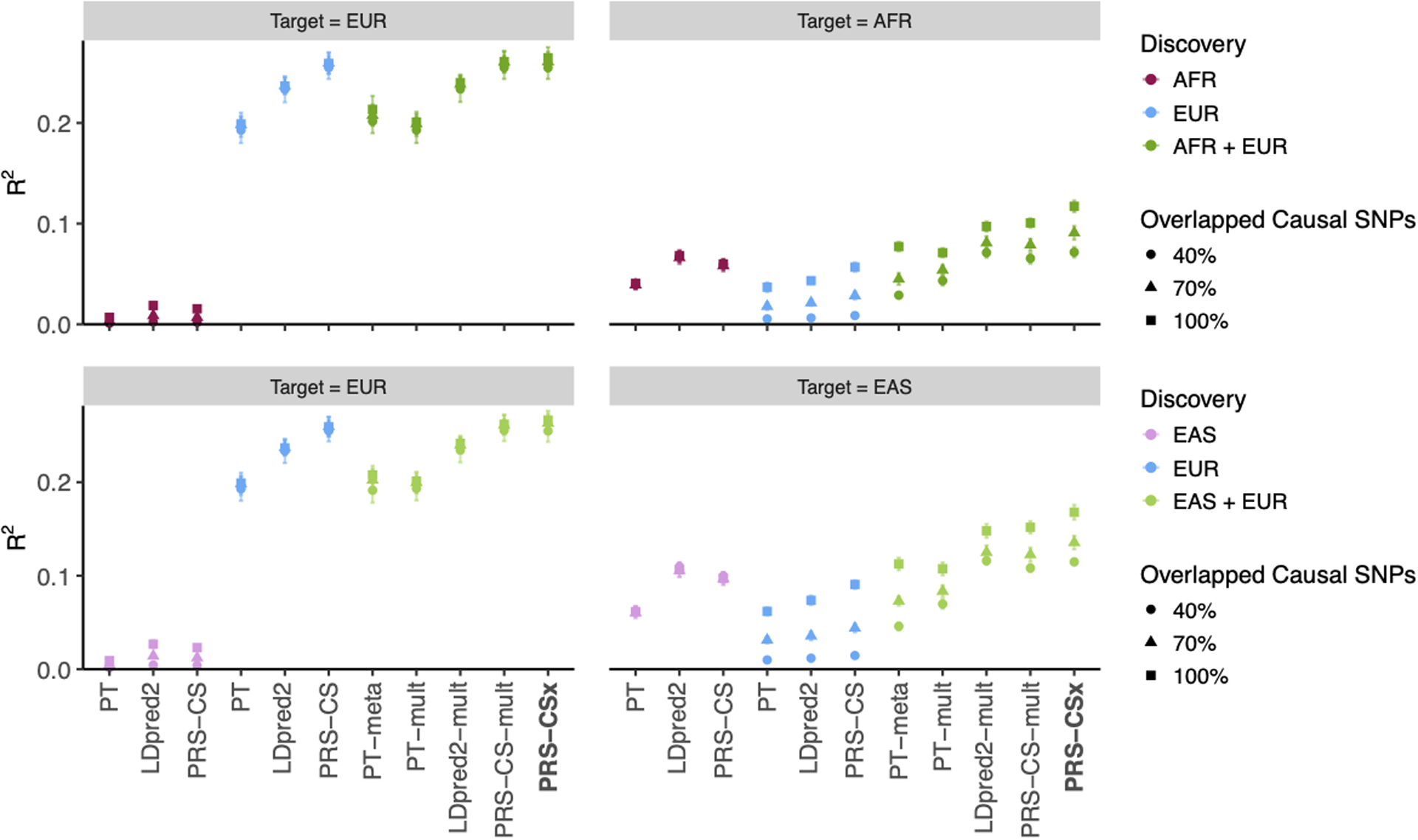
Phenotypes were simulated using 1% of randomly sampled causal variants. 100%, 70% or 40% of the causal variants were shared across populations. Shared causal variants had a cross-population genetic correlation of 0.7. SNP heritability was fixed at 50%. PRS were trained using 100K EUR samples and 20K non-EUR (EAS or AFR) samples. Numerical results are reported in Supplementary Table 7.

Extended Data Fig. 7. Prediction accuracy of different polygenic prediction methods when SNP effect sizes are minor allele frequency (MAF) and linkage disequilibrium (LD) dependent.

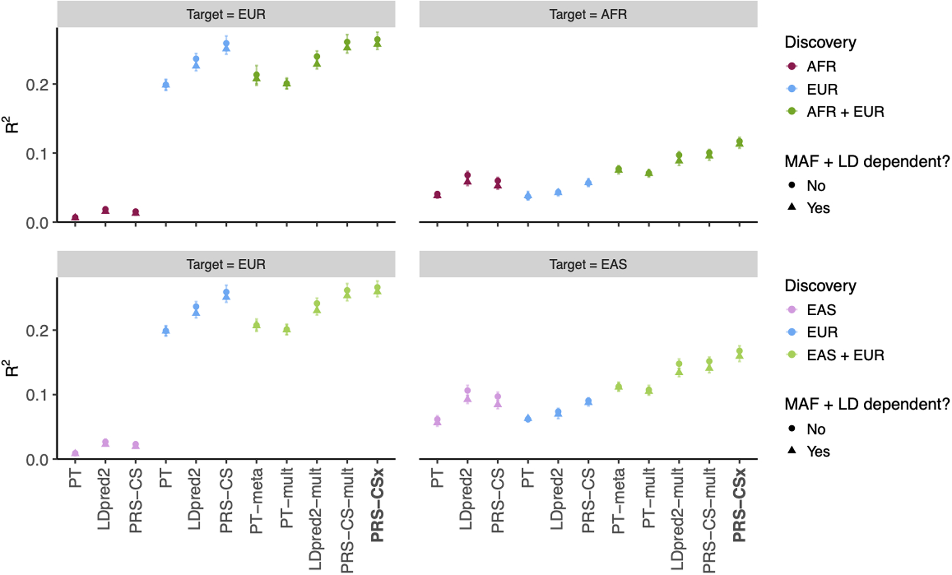
Phenotypes were simulated using 1% of randomly sampled causal variants (shared across populations), a cross-population genetic correlation of 0.7, and SNP heritability of 50%. SNP effect sizes were dependent on MAF and LD scores such that SNPs with lower MAF and located in lower LD regions tended to have larger effect sizes. PRS were trained using 100K EUR samples and 20K non-EUR (EAS or AFR) samples. Numerical results are reported in Supplementary Table 8.

Extended Data Fig. 8. Relative prediction accuracy for quantitative traits across target populations.

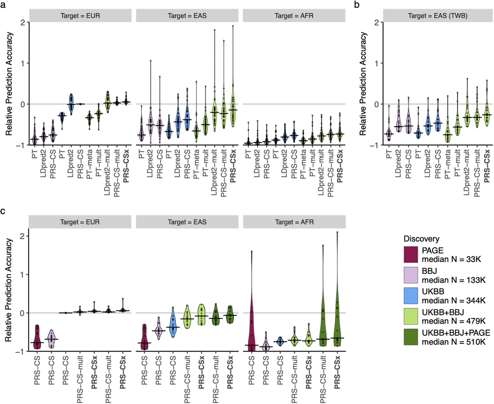
Relative prediction performance for single-discovery and multi-discovery PRS construction methods using discovery GWAS summary statistics a, from UKBB and BBJ, across 33 traits, in different UKBB target populations (EUR, EAS and AFR); b, from UKBB and BBJ, across 21 traits, in the Taiwan Biobank (TWB); c, from UKBB, BBJ and PAGE, across 14 traits, in different UKBB target populations (EUR, EAS and AFR). Each data point shows the relative increase of prediction performance, defined as R²/R²_{PRS-CS (UKBB)-EUR} - 1, in which R²_{PRS-CS (UKBB)-EUR} is the R² of the trait in the EUR population using PRS-CS trained on the UKBB GWAS summary statistics. In UKBB target populations (panels a and c), R² were averaged across 100 random splits of the target samples into validation and testing datasets. The crossbar indicates the median of the relative increase of predictive performance across the traits examined. “median N” indicates the median sample size across the respective discovery GWAS.

Extended Data Fig. 9. Trace plots and autocorrelation functions (ACFs) for assessing the convergence and mixing of the Gibbs sampler used in PRS-CSx.

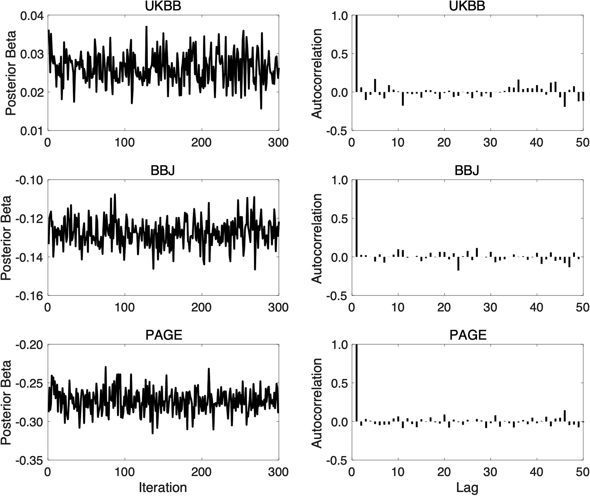
Left panels: Trace plots, after discarding the burn-in iterations and thinning the Markov chain by a factor of 5, for the posterior effects of rs7412 on low-density lipoprotein cholesterol when integrating UKBB, BBJ and PAGE GWAS summary statistics using PRS-CSx. Right panels: The autocorrelation functions (ACFs) for the traces shown on the left.

STANLEY GLOBAL ASIA INIATIVES

Yong Min Ahn¹⁸, Kazufumi Akiyama¹⁹, Makoto Arai²⁰, Ji Hyun Baek²¹, Wei J. Chen²², Young-Chul Chung²³, Gang Feng²⁴, Kumiko Fujii²⁵, Stephen J. Glatt^26,27, Zhenglin Guo¹, Kyooseob Ha¹⁸, Kotaro Hattori²⁸, Teruhiko Higuchi²⁹, Akitoyo Hishimoto³⁰, Kyung Sue Hong²¹, Yasue Horiuchi²⁰, Hailiang Huang^1,8,16,60, Hai-Gwo Hwu³¹, Masashi Ikeda³², Sayuri Ishiwata²⁸, Masanari Itokawa²⁰, Nakao Iwata³², Eun-Jeong Joo³³, Rene Kahn³⁴, Sung-Wan Kim³⁵, Se Joo Kim³⁶, Se Hyun Kim¹⁸, Makoto Kinoshita³⁷, Hiroshi Kunugi²⁸, Agung Kusumawardhani³⁸, Jimmy Lee^39,40, Byung Dae Lee⁴¹, Heon-Jeong Lee⁴², Jianjun Liu^43,44, Ruize Liu^1,8, Xiancang Ma⁴⁵, Woojae Myung⁴⁶, Shusuke Numata³⁷, Tetsuro Ohmori³⁷, Ikuo Otsuka^30,47, Yuji Ozeki²⁵, Shengying Qin^2,60, Yunfeng Ruan^1,2, Akira Sawa¹⁵, Sibylle G. Schwab^48,49, Wenzhao Shi²⁴, Kazutaka Shimoda⁵⁰, Kang Sim³⁹, Ichiro Sora³⁰, Jinsong Tang^51,52,53,54, Tomoko Toyota⁵⁵, Ming Tsuang⁵⁶, Dieter B. Wildenauer⁵⁷, Hong-Hee Won⁵⁸, Takeo Yoshikawa⁵⁵, Alice Zheng¹, Feng Zhu⁵⁹

¹⁸Department of Psychiatry, Seoul National University Hospital, Seoul, Korea. ¹⁹Department of Biological Psychiatry and Neuroscience, Dokkyo Medical University School of Medicine, Mibu, Japan. ²⁰Department of Psychiatry and Behavioral Sciences, Tokyo Metropolitan Institute of Medical Science, Tokyo, Japan. ²¹Department of Psychiatry, Sungkyunkwan University, Samsung Medical Center, Seoul, Korea. ²²Department of Psychiatry, National Taiwan University Hospital and College of Medicine, National Taiwan University, Taipei, Taiwan. ²³Department of Psychiatry, Chonbuk National University Medical School, Jeonbuk, Korea. ²⁴Digital Health China Technologies Co., China. ²⁵Department of Psychiatry, Shiga University of Medical Science, Shiga, Japan. ²⁶Department of Psychiatry & Behavioral Sciences, SUNY Upstate Medical University, Syracuse, NY, USA. ²⁷Department of Neuroscience & Physiology, SUNY Upstate Medical University, Syracuse, NY, USA. ²⁸National Institute of Neuroscience, National Center of Neurology and Psychiatry, Tokyo, Japan. ²⁹National Center of Neurology and Psychiatry, Tokyo, Japan. ³⁰Department of Psychiatry, Kobe University Graduate School of Medicine, Tokyo, Japan. ³¹Department of Psychiatry, National Taiwan University, Taipei, Taiwan. ³²Department of Psychiatry, Fujita Health University School of Medicine, Toyoake, Japan. ³³Department of Neuropsychiatry, School of Medicine, Eulji University, Daejeon, Korea. ³⁴Department of Psychiatry, Icahn School of Medicine at Mount Sinai, New York, NY, USA. ³⁵Department of Psychiatry, Chonnam National University Medical School, Gwangju, Korea. ³⁶Department of Psychiatry, Yonsei University College of Medicine, Seoul, Korea. ³⁷Department of Psychiatry, Institute of Biomedical Sciences, Tokushima University Graduate School, Tokushima, Japan. ³⁸Department of Psychiatry, University of Indonesia, Jakarta, Indonesia. ³⁹Institute of Mental Health, Singapore, Singapore. ⁴⁰Lee Kong Chian School of Medicine, Nanyang Technological University, Singapore, Singapore. ⁴¹Department of Psychiatry, Pusan National University Hospital, Busan, Korea. ⁴²Department of Psychiatry, Korea University College of Medicine, Seoul, Korea. ⁴³Genome Institute of Singapore, A*STAR, Singapore, Singapore. ⁴⁴Yong Loo Lin School of Medicine, National University of Singapore, Singapore, Singapore. ⁴⁵Department of Psychiatry, The First Affiliated Hospital of Xi’an Jiaotong University, Xi’an, China. ⁴⁶Department of Psychiatry, Seoul National University Bundang Hospital, Seongnam, Korea. ⁴⁷Laboratory for Statistical Analysis, RIKEN Center for Integrative Medical Sciences, Yokohama, Japan. ⁴⁸School of Chemistry and Molecular Bioscience,University of Wollongong, Wollongong, Australia. ⁴⁹Illawarra Health and Medical Research Institute, Wollongong, Australia. ⁵⁰Department of Psychiatry, Dokkyo Medical University School of Medicine, Mibu, Japan. ⁵¹Department of Psychiatry, Sir Run Run Shaw Hospital, Zhejiang University School of Medicine, Hangzhou, Zhejiang, China. ⁵²Key Laboratory of Medical Neurobiology of Zhejiang Province, Hangzhou, Zhejiang, China. ⁵³Department of Psychiatry, the Second Xiangya Hospital, Central South University, Changsha, Hunan, China. ⁵⁴National Clinical Research Center on Mental Disorders, Changsha, Hunan, China. ⁵⁵Laboratory for Molecular Psychiatry, RIKEN Center for Brain Science, Wako, Japan. ⁵⁶Department of Psychiatry, University of California San Diego, San Diego, CA, USA. ⁵⁷University of Western Australia, Perth, Australia. ⁵⁸Samsung Advanced Institute for Health Sciences and Technology (SAIHST), Sungkyunkwan University, Samsung Medical Center, Seoul, Korea. ⁵⁹Center for Translational Medicine, The First Affiliated Hospital of Xi’an Jiaotong University, Xi’an, China.

DATA AVAILABILITY

Publicly available data are available from the following sites: 1KG Phase 3 reference panels: https://mathgen.stats.ox.ac.uk/impute/1000GP_Phase3.html; Genetic map for each subpopulation: ftp.1000genomes.ebi.ac.uk/vol1/ftp/technical/working/20130507_omni_recombination_rates; UKBB summary statistics: http://www.nealelab.is/uk-biobank (“GWAS round 2” was used in this study); BBJ summary statistics were downloaded from PheWeb: https://pheweb.jp; PAGE summary statistics were downloaded from the GWAS Catalog: https://www.ebi.ac.uk/gwas/downloads/summary-statistics; PGC wave 2 schizophrenia GWAS (49 EUR cohorts): https://www.med.unc.edu/pgc/download-results/;

Leave-one-out schizophrenia EAS summary statistics are available upon request to the Schizophrenia Working Group of the PGC (https://www.med.unc.edu/pgc/pgc-workgroups/schizophrenia/). These leave-one-out summary statistics are under controlled access per the data use limitation imposed by compliance, participant consent and/or national laws. Application to access such data requires a short research proposal that will go through PGC’s review and approval process. This process takes two weeks. Individual-level schizophrenia data of East Asian ancestry are available upon application to the Stanley Global Asia Initiatives: SGAI@broadinstitute.org. These data must be under controlled access due to the data use limitation imposed by the compliance, participant consent and national laws. Application to access such data requires a short research proposal that will be reviewed by PI of the constituent study, and if necessary, by the respective ethic committee. The PI review process takes two weeks. Taiwan Biobank data used in this study contain protected health information and are thus under controlled access. Application to access such data can be made to the Taiwan Biobank (https://www.twbiobank.org.tw/new_web_en/). Posterior SNP effect size estimates generated by PRS-CSx for the traits examined in this work: https://github.com/getian107/PRScsx.

REFERENCES

- 1.Khera AV et al. Genome-wide polygenic scores for common diseases identify individuals with risk equivalent to monogenic mutations. Nat. Genet 50, 1219–1224 (2018). [DOI] [PMC free article] [PubMed] [Google Scholar]
- 2.Khera AV et al. Polygenic prediction of weight and obesity trajectories from birth to adulthood. Cell 177, 587–596.e9 (2019). [DOI] [PMC free article] [PubMed] [Google Scholar]
- 3.Torkamani A, Wineinger NE & Topol EJ The personal and clinical utility of polygenic risk scores. Nat. Rev. Genet 19, 581–590 (2018). [DOI] [PubMed] [Google Scholar]
- 4.Chatterjee N, Shi J & García-Closas M Developing and evaluating polygenic risk prediction models for stratified disease prevention. Nat. Rev. Genet 17, 392–406 (2016). [DOI] [PMC free article] [PubMed] [Google Scholar]
- 5.Zheutlin AB et al. Penetrance and pleiotropy of polygenic risk scores for schizophrenia in 106,160 patients across four health care systems. Am. J. Psychiatry 176, 846–855 (2019). [DOI] [PMC free article] [PubMed] [Google Scholar]
- 6.Lambert SA, Abraham G & Inouye M Towards clinical utility of polygenic risk scores. Hum. Mol. Genet 28, R133–R142 (2019). [DOI] [PubMed] [Google Scholar]
- 7.Martin AR et al. Clinical use of current polygenic risk scores may exacerbate health disparities. Nat. Genet 51, 584–591 (2019). [DOI] [PMC free article] [PubMed] [Google Scholar]
- 8.Martin AR et al. Human demographic history impacts genetic risk prediction across diverse populations. Am. J. Hum. Genet 100, 635–649 (2017). [DOI] [PMC free article] [PubMed] [Google Scholar]
- 9.Wang Y et al. Theoretical and empirical quantification of the accuracy of polygenic scores in ancestry divergent populations. Nat. Commun 11, 3865 (2020). [DOI] [PMC free article] [PubMed] [Google Scholar]
- 10.Duncan L et al. Analysis of polygenic risk score usage and performance in diverse human populations. Nat. Commun 10, 1–9 (2019). [DOI] [PMC free article] [PubMed] [Google Scholar]
- 11.Popejoy AB & Fullerton SM Genomics is failing on diversity. Nature 538, 161–164 (2016). [DOI] [PMC free article] [PubMed] [Google Scholar]
- 12.Sirugo G, Williams SM & Tishkoff SA The missing diversity in human genetic studies. Cell 177, 26–31 (2019). [DOI] [PMC free article] [PubMed] [Google Scholar]
- 13.Hindorff LA et al. Prioritizing diversity in human genomics research. Nat. Rev. Genet 19, 175–185 (2018). [DOI] [PMC free article] [PubMed] [Google Scholar]
- 14.Peterson RE et al. Genome-wide association studies in ancestrally diverse populations: opportunities, methods, pitfalls, and recommendations. Cell 179, 589–603 (2019). [DOI] [PMC free article] [PubMed] [Google Scholar]
- 15.Lam M et al. Comparative genetic architectures of schizophrenia in East Asian and European populations. Nat. Genet 51, 1670–1678 (2019). [DOI] [PMC free article] [PubMed] [Google Scholar]
- 16.Brown BC, Ye CJ, Price AL & Zaitlen N Transethnic genetic-correlation estimates from summary statistics. Am. J. Hum. Genet 99, 76–88 (2016). [DOI] [PMC free article] [PubMed] [Google Scholar]
- 17.Shi H et al. Localizing Components of Shared Transethnic Genetic Architecture of Complex Traits from GWAS Summary Data. Am. J. Hum. Genet 106, 805–817 (2020). [DOI] [PMC free article] [PubMed] [Google Scholar]
- 18.Shi H et al. Population-specific causal disease effect sizes in functionally important regions impacted by selection. Nat. Commun 12, 1098–15 (2021). [DOI] [PMC free article] [PubMed] [Google Scholar]
- 19.Ge T, Chen C-Y, Ni Y, Feng Y-CA & Smoller JW Polygenic prediction via Bayesian regression and continuous shrinkage priors. Nat. Commun 10, 1776 (2019). [DOI] [PMC free article] [PubMed] [Google Scholar]
- 20.Privé F, Arbel J & Vilhjalmsson BJ LDpred2: better, faster, stronger. Bioinformatics 36, 5424–5431 (2020). [DOI] [PMC free article] [PubMed] [Google Scholar]
- 21.Vilhjalmsson BJ et al. Modeling linkage disequilibrium increases accuracy of polygenic risk scores. Am. J. Hum. Genet 97, 576–592 (2015). [DOI] [PMC free article] [PubMed] [Google Scholar]
- 22.Lloyd-Jones LR et al. Improved polygenic prediction by Bayesian multiple regression on summary statistics. Nat. Commun 10, 5086 (2019). [DOI] [PMC free article] [PubMed] [Google Scholar]
- 23.Mak TSH, Porsch RM, Choi SW, Zhou X & Sham PC Polygenic scores via penalized regression on summary statistics. Genet. Epidemiol 41, 469–480 (2017). [DOI] [PubMed] [Google Scholar]
- 24.Coram MA, Fang H, Candille SI, Assimes TL & Tang H Leveraging multi-ethnic evidence for risk assessment of quantitative traits in minority populations. Am. J. Hum. Genet 101, 218–226 (2017). [DOI] [PMC free article] [PubMed] [Google Scholar]
- 25.Grinde KE et al. Generalizing polygenic risk scores from Europeans to Hispanics/Latinos. Genet. Epidemiol 43, 50–62 (2019). [DOI] [PMC free article] [PubMed] [Google Scholar]
- 26.Marquez-Luna C, Loh P-R, South Asian Type 2 Diabetes (SAT2D) Consortium, SIGMA Type 2 Diabetes Consortium & Price, A. L. Multiethnic polygenic risk scores improve risk prediction in diverse populations. Genet. Epidemiol 41, 811–823 (2017). [DOI] [PMC free article] [PubMed] [Google Scholar]
- 27.Weissbrod O et al. Leveraging fine-mapping and non-European training data to improve trans-ethnic polygenic risk scores. medRxiv (2021). doi: 10.1101/2021.01.19.21249483 [DOI] [Google Scholar]
- 28.Sudlow C et al. UK Biobank: an open access resource for identifying the causes of a wide range of complex diseases of middle and old age. PLoS Med. 12, e1001779 (2015). [DOI] [PMC free article] [PubMed] [Google Scholar]
- 29.Kanai M et al. Genetic analysis of quantitative traits in the Japanese population links cell types to complex human diseases. Nat. Genet 50, 390–400 (2018). [DOI] [PubMed] [Google Scholar]
- 30.Sakaue S et al. A global atlas of genetic associations of 220 deep phenotypes. medRxiv (2021). doi: 10.1101/2020.10.23.20213652 [DOI] [Google Scholar]
- 31.Wojcik GL et al. Genetic analyses of diverse populations improves discovery for complex traits. Nature 570, 514–518 (2019). [DOI] [PMC free article] [PubMed] [Google Scholar]
- 32.Chen C-Y et al. Analysis across Taiwan Biobank, Biobank Japan and UK Biobank identifies hundreds of novel loci for 36 quantitative traits. medRxiv (2021). doi: 10.1101/2021.04.12.21255236 [DOI] [PubMed] [Google Scholar]
- 33.Feng Y-CA et al. Taiwan Biobank: a rich biomedical research database of the Taiwanese population. medRxiv (2021). doi: 10.1101/2021.12.21.21268159 [DOI] [PMC free article] [PubMed] [Google Scholar]
- 34.Schizophrenia Working Group of the Psychiatric Genomics Consortium. Biological insights from 108 schizophrenia-associated genetic loci. Nature 511, 421–427 (2014). [DOI] [PMC free article] [PubMed] [Google Scholar]
- 35.International Schizophrenia Consortium et al. Common polygenic variation contributes to risk of schizophrenia and bipolar disorder. Nature 460, 748–752 (2009). [DOI] [PMC free article] [PubMed] [Google Scholar]
- 36.1000 Genomes Project Consortium et al. A global reference for human genetic variation. Nature 526, 68–74 (2015). [DOI] [PMC free article] [PubMed] [Google Scholar]
- 37.Su Z, Marchini J & Donnelly P HAPGEN2: simulation of multiple disease SNPs. Bioinformatics 27, 2304–2305 (2011). [DOI] [PMC free article] [PubMed] [Google Scholar]
- 38.Gelman A & Rubin DB Inference from iterative simulation using multiple sequences. Stat. Sci 7, 457–472 (1992). [Google Scholar]
- 39.Ge T et al. Validation of a trans-ancestry polygenic risk score for type 2 diabetes in diverse populations. medRxiv (2021). doi: 10.1101/2021.09.11.21263413 [DOI] [PMC free article] [PubMed] [Google Scholar]
- 40.Majara L et al. Low generalizability of polygenic scores in African populations due to genetic and environmental diversity. bioRxiv (2021). doi: 10.1101/2021.01.12.426453 [DOI] [Google Scholar]
- 41.Atkinson EG et al. Tractor uses local ancestry to enable the inclusion of admixed individuals in GWAS and to boost power. Nat. Genet 53, 195–204 (2021). [DOI] [PMC free article] [PubMed] [Google Scholar]
- 42.Maples BK, Gravel S, Kenny EE & Bustamante CD RFMix: a discriminative modeling approach for rapid and robust local-ancestry inference. Am. J. Hum. Genet 93, 278–288 (2013). [DOI] [PMC free article] [PubMed] [Google Scholar]
- 43.Berisa T & Pickrell JK Approximately independent linkage disequilibrium blocks in human populations. Bioinformatics 32, 283–285 (2016). [DOI] [PMC free article] [PubMed] [Google Scholar]
- 44.Choi SW & O’Reilly PF PRSice-2: Polygenic Risk Score software for biobank-scale data. GigaScience 8, 2091 (2019). [DOI] [PMC free article] [PubMed] [Google Scholar]
- 45.Chang CC et al. Second-generation PLINK: rising to the challenge of larger and richer datasets. GigaScience 4, 7 (2015). [DOI] [PMC free article] [PubMed] [Google Scholar]
- 46.Zeng J et al. Signatures of negative selection in the genetic architecture of human complex traits. Nat. Genet 360, 1411–753 (2018). [DOI] [PubMed] [Google Scholar]
- 47.Gazal S et al. Linkage disequilibrium-dependent architecture of human complex traits shows action of negative selection. Nat. Genet 49, 1421–1427 (2017). [DOI] [PMC free article] [PubMed] [Google Scholar]
- 48.Speed D, Holmes J & Balding DJ Evaluating and improving heritability models using summary statistics. Nat. Genet 52, 458–462 (2020). [DOI] [PubMed] [Google Scholar]
- 49.Bulik-Sullivan BK et al. LD Score regression distinguishes confounding from polygenicity in genome-wide association studies. Nat. Genet 47, 291–295 (2015). [DOI] [PMC free article] [PubMed] [Google Scholar]
- 50.Lam M et al. RICOPILI: Rapid Imputation for COnsortias PIpeLIne. Bioinformatics 36, 930–933 (2020). [DOI] [PMC free article] [PubMed] [Google Scholar]
Associated Data
This section collects any data citations, data availability statements, or supplementary materials included in this article.
Supplementary Materials
Data Availability Statement