Abstract
Drug repurposing is an effective strategy to identify new uses for existing drugs, providing the quickest possible transition from bench to bedside. Real-world data, such as electronic health records and insurance claims, provide information on large cohorts of users for many drugs. Here we present an efficient and easily customized framework for generating and testing multiple candidates for drug repurposing using a retrospective analysis of real-world data. Building upon well-established causal inference and deep learning methods, our framework emulates randomized clinical trials for drugs present in a large-scale medical claims database. We demonstrate our framework on a coronary artery disease cohort of millions of patients. We successfully identify drugs and drug combinations that substantially improve the coronary artery disease outcomes but haven’t been indicated for treating coronary artery disease, paving the way for drug repurposing.
Drug repurposing (also known as, drug repositioning) is a strategy to accelerate the drug discovery process by identifying novel uses for existing approved drugs1. The primary advantage of drug repurposing over traditional drug development is that it starts from compounds with well-characterized pharmacology and safety profiles and can substantially reduce the risk of adverse effects and attrition in clinical phases2.
While many successful repurposed drugs (for example, Viagra for erectile dysfunction) have been discovered serendipitously3, computation-based repurposing methods have developed recently by leveraging structural features of compounds or proteins4,5, genome-wide association study (GWAS)6, transcriptional responses7 and gene expression8. These methods focus primarily on using pre-clinical information. Unfortunately, the clinical therapeutic effects in humans are not always consistent with pre-clinical outcomes9.
In healthcare, real-world data (RWD)10 refers to longitudinal observational data derived from sources that are associated with outcomes in a heterogeneous patient population in real-world settings, such as patient surveys, electronic health records (EHRs), and claims and billing activities. Since RWD are direct observations from human bodies, they become a promising source for drug repurposing. A few researchers have already validated a small number of repurposing drug candidates on RWD11,12. However, there are some limitations with these approaches. First, most studies are complementary (that is, the original hypotheses usually come from other studies). Second, their studied number of repurposing candidates is limited and unable to proactively generate de novo repurposing drug candidates.
In this study, we follow protocols of randomized clinical trial (RCT) design13, and computationally screen repurposing candidates for beneficial effect by explicitly emulating the corresponding clinical trials using RWD. Considering the inherent characteristics of RWD (that is, temporal sequence data and existing confounding variables14), we apply deep learning and causal inference methodologies to control the confounders in RWD, and systematically estimate the drug effects on various disease outcomes. Specifically, the estimated drug effects are obtained by long short-term memory (LSTM)15 and inverse probability of treatment weighting (IPTW)16, on MarketScan claims data17.
As a test case, we apply the proposed drug repurposing framework to a coronary artery disease (CAD) cohort of millions of patients and emulate RCTs for multiple drug candidates, estimating their effects on CAD progression outcomes.
In general, our contribution is threefold:
We develop a framework for high-throughput screening of on-market drugs by emulating, for each drug, an RCT that evaluates its beneficial effect. This allows repurposed drug candidates to be proactively generated from existing large-scale RWD.
We present an innovative study design for the estimation of a drug’s effect from longitudinal observational data. The CAD cohorts are automatically derived under our framework, which accelerates the process of computational drug repurposing.
We propose a propensity score estimation model based on deep learning to correct for confounding and selection biases. Experimental comparisons to the logistic-regression-based propensity score estimation model show that our proposed deep learning model effectively estimates drug effects from RWD, paving the way for drug repurposing.
We evaluate the therapeutic effect of drug combinations, drug-class-levelled candidates on disease outcomes and further explore potential repurposing opportunities with different model parameters. We also compare our framework with three existing pre-clinical drug repurposing methods, which gives a favourable outcome.
Overall framework
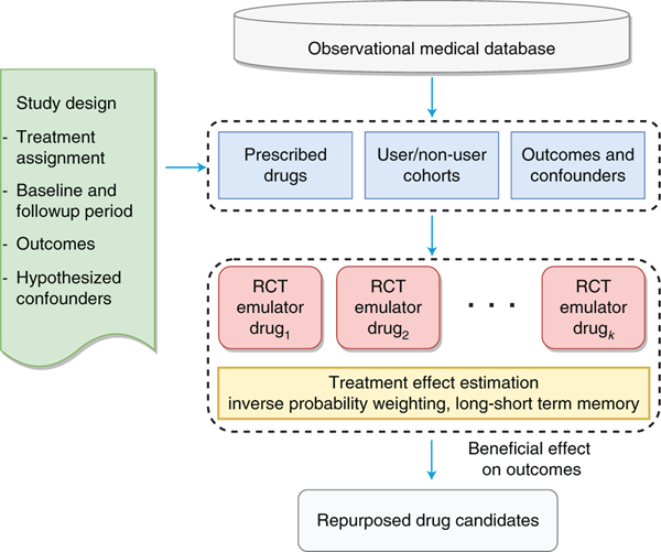
We develop a high-throughput, computational drug-repurposing pipeline (Fig. 1) that, given a disease cohort (for example, CAD patients), extracts a list of potential repurposing drug ingredients and, for each, identifies the corresponding user and non-user sub-cohorts. It then computes, for all patients in both sub-cohorts, a large number of features (confounding factors), as well as disease progression outcomes. The treatment effects are estimated after correcting for confounding and selection biases using the deep learning framework (Fig. 2). The framework is equipped with an attention mechanism that provides interpretability for the model. Drug ingredients with statistically significant beneficial effects will be considered as repurposed drug candidates and suggested as treatments for CAD. This algorithm shows an overview of the steps in estimating the effect of assigned treatment on the outcome from observational data:
Fig. 1 |. Flowchart of overall drug repurposing framework.
First, a list of potential repurposing drug ingredients are extracted from the observational medical database given a disease cohort. Second, for each ingredient, the framework identifies the corresponding user and non-user sub-cohorts, and computes a large number of features for patients in both sub-cohorts. Third, the treatment effects are estimated via emulating an RCT for each ingredient to adjust confounding and biases.
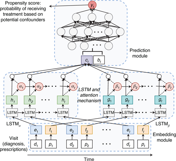
Fig. 2 |. Illustration of the deep learning model for predicting treatment probability (or propensity score) that we used to correct confounding from time sequence data (including diagnoses dt, prescriptions pt and demographics bt).
It consists of three main components: an embedding module, a recurrent neural network (LSTM) and a prediction module.
Input: patient data: assigned treatment, outcomes, values for potential confounders
Output: repurposed drug candidates, and their estimated effect, unbalanced feature ratio and significance
Generate user and non-user sub-cohorts for the treatment
C ompute balancing weights for all patients in both sub-cohorts via LSTM-based IPTW
Estimate the effect over multiple outcomes after correcting for the biases in the confounders (equation (1))
Compute the unbalanced feature ratio for the treatment after re-weighting using standardized difference (equation (2))
Estimate the significance of effect and compute adjusted p-values using bootstrapping
if estimated effect < 0 and adjusted p-value < 0.05 and unbalanced feature ratio < 2% then
return the estimated effect, unbalanced feature ratio and computed p-value
end if
Results
In this section we introduce the dataset we use for this study and then demonstrate the performance of our model in CAD drug repurposing experiments.
Dataset.
We identified around 107.5 million distinct patients in the MarketScan Commercial Claims and Encounters (CCAE)17 from 2012 to 2017, which contain individual-level, de-identified healthcare claims information from employers, health plans and hospitals. CCAE contains the largest number of patients and the most diverse population of the MarketScan data. The MartketScan table structure and data flow can be found in its user manual18. We extracted patient data from three source tables: Outpatient Drug (D), Inpatient Admission (I) and Outpatient Services (O). Then we compiled and formulated the raw data into five separate tables that can be easily prepossessed. The details of these tables and demo input data can be found in our Github repository at https://github.com/ruoqi-liu/DeepIPW.
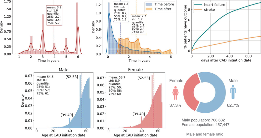
MarketScan claims data are primarily used for evaluating health utilization and services. The overall distribution of patients during the recording period is shown in Extended Data Fig. 1a. We consider both inpatient and outpatient claims. CAD cohort criteria are defined using International Classification of Diseases (ICD) codes19 (Supplementary Table 1). In total, there were 1,178,997 CAD patients. We refer to the first date when patients were diagnosed with CAD as their CAD initiation date. Extended Data Fig. 1b shows the patient distribution of time before/after CAD initiation date.
We identify three categories of study variable: demographic characteristics, diagnosis codes and prescription medication. Demographic characteristics in MarketScan CAD data include information on age and gender for each patient. Extended Data Fig. 1d shows the age and gender statistics distributions of our dataset. Because a majority of the data come from commercial claims, race and ethnicity information is incomplete and is not included in the analysis. Diagnosis codes in MarketScan CAD data are defined using the ICD codes for billing purposes. There are 57,089 ICD-9/10 codes considered in the dataset. Prescription medications in MarketScan CAD data also contain all prescription drug claims, which contain prescription drug name (generic and brand), national drug code (NDC) and the number of days of supply approved. By matching NDCs to observational medical outcomes partnership (OMOP) ingredient concept IDs20, we get 1,353 unique drugs in the dataset for drug repositioning screening. For drugs with multiple ingredients, we consider each active ingredient separately in the mapping processes.
To evaluate the drug effect, we consulted domain experts to define a set of clinically relevant events linked to CAD as the disease outcomes (for example, heart failure onset and stroke onset). These definitions are based on ICD codes and can be found in Supplementary Tables 2 and 3. Since CAD is the major risk factor for both heart failure21,22 and stroke23,24, we hypothesize that an effective drug will lower the risks of CAD patients developing those diseases. Extended Data Fig. 1c demonstrates the time to develop outcomes from the CAD initiation date. The confounding variables affect both treatment assignment of patients and an outcome used in the trial. We consult domain experts to compile a list of hypothesized confounders for the CAD case study with respect to the study variables illustrate above: demographics, co-morbidities (diagnosis codes) and co-prescribed drugs.
Model performance.
Evaluation metrics.
Treatment effect estimation.
In this study, we leverage average treatment effect (ATE) to examine the treatment effect at the population level, which is defined as
| (1) |
where and are the expected potential treated and control outcomes of the whole population, respectively. The values of ATE are used to determine whether the given treatment can improve disease outcomes or not.
Testing feature balance.
We evaluate the performance of models by measuring features’ balance between the weighted user and non-user sub-cohorts generated by the IPTW. Given patient weights from IPTW, we quantify the balance for each feature using its standardized mean difference (SMD), which is the difference in the variable means between the two treatment groups, divided by the combined standard deviation. To be exact, we use the following definition for standardized difference:
| (2) |
where μuser and μnon-user are the mean in user cohort and non-user cohort; suser2 and snon–user2 are sample variance of variables in two s2 is calculated by sub-cohorts. For binary variables, the variance . We consider a standardized difference greater than 0.1 as unbalanced25 and compute the unbalanced feature ratio (that is, unbalanced/all features) before and after weighting to evaluate the performance of balancing. The user and non-user sub-cohorts are considered as balanced if their unbalanced feature ratio is below 2% after weighting.
Confidence intervals and significance of effect.
We use bootstrapping26 to calculate the confidence intervals of estimators of and , and statistical significance of ATE. For each candidate I ingredient, we repeatedly generate multiple different control drugs via random sampling with replacement, and the analysis is repeated in each bootstrap sample. The 95% confidence interval is then computed by using the standard normal approximation: ±1.96 times the estimate of the standard error. The p-value of the effect estimator can be computed by the normal cumulative distribution function of estimators. We use adjusted p-value27 as a statistically significant measurement. We consider a repurposing drug candidate as significant if its adjusted p-value is below 0.05.
Performance over repurposing drug candidates.
We identified 55 qualified drugs following our study design (Methods). Then we estimated the treatment effect on various disease outcomes (that is, heart failure and stroke). The flowchart of data collection and study process can be found in Supplementary Fig. 2.
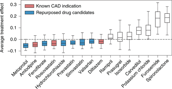
Among the qualified drugs obtained from the data, four of them are known CAD treatments: amlodipine, diltiazem, ticagrelor and rosuvastatin (drug label information is collected from SIDER28 and DrugBank29). Our framework successfully retrieved three of these known drugs: amlodipine, diltiazem and rosuvastatin. We demonstrate the distribution of estimated ATE in Fig. 3. Here, we show the drug candidates with balanced user and non-user sub-cohorts after re-weighting and statistically significant estimates (adjusted p-value). All the drugs are ranked from left to right according to increasing estimated ATE values. Based on the definition of ATE (that is, the weighted average of observed outcomes from the user and non-user sub-cohorts), the drug ingredients with ATE values smaller than 0 are identified as improving disease outcomes, while the drug ingredients with ATE values larger than 0 are identified to worsen disease outcomes. For drugs with beneficial effects, we colour those with known CAD indications in red and those without in blue.
Fig. 3 |. Distribution of estimated ATE of drugs on defined outcomes across the 50 bootstrap samples.
All shown drugs satisfy two conditions: adjusted p-value ≤ 0.05 and post-weighting unbalanced ratio ≤ 2%. Within the boxplot, the central line denotes the median, and the bottom and the top edges denote the 25th (Q1) and 75th (Q3) and percentiles respectively. The whiskers extend to 1.5 times the interquartile range.
From the results, we observe that nine drugs yield a beneficial effect on disease outcomes among the sixteen selected significant drug candidates. Specifically, only three have been indicated for CAD according to their drug labels information. The remaining six drugs, which have not been indicated for treating CAD but can improve the disease outcomes, are considered as repurposed drug candidates. We find evidence to support these six drug candidates from related literature and web resources as follows: (1) metoprolol is one of the most commonly used beta-blockers for treating high blood pressure and chest pain. It shows beneficial effects in patients with heart failure associated with CAD30; (2) fenofibrate is mainly used to treat abnormal blood lipid levels and also appears to decrease the risk of CAD in patients with diabetes mellitus31; (3) hydrochlorothiazide, which is often used to treat high blood pressure and diabetes insipidus32, also shows effectiveness in preventing CAD33; (4) pravastatin has also shown a beneficial effect on CAD34; (5) for simvastatin, results from RCTs show that it can reduce the occurrence of heart failure in patients with CAD35; (6) valsartan, a kind of angiotensin receptor blocker, results in improved coronary micro-vascular flow reserve, suggesting a direct benefit in hypertensive patients with stable CAD36.
We further list the sub-cohort size, feature balancing and estimated ATE values for each drug candidate in Table 1. The results of all 55 drugs can be found in Supplementary Table 4. The first column lists the names corresponding to drugs in Fig. 3. The second and third columns denote the number of patients in user and non-user sub-cohorts, respectively. The next two columns denote the average number of unbalanced covariates before and after re-weighting. The unbalanced ratio column represents the ratio of unbalanced covariates to all covariates after re-weighting (that is, the number of unbalanced covariates divided by the total number of covariates). And the last two columns are the estimated ATE before and after re-weighting. We rank the drugs by increasing re-weighted ATE values. We see that our proposed method successfully corrects for most biases in the original data, which results in a decrease in the number of unbalanced covariates.
Table 1 |.
The estimated treatment effects for CAD over balanced and statistically significant drug ingredients
| Drug name | Users | Non-users | Unbalanced covariates (pre) | Unbalanced covariates (post) | Covariates | Unbalanced ratio (post) | ATE (pre) | ATE (post) |
|---|---|---|---|---|---|---|---|---|
| Metoprolol | 9,730 | 29,190 | 38.308 | 23.231 | 1,270 | 1.8 | −0.023 | −0.043 |
| Fenofibrate | 1,352 | 4,056 | 39.340 | 13.200 | 1,038 | 1.3 | −0.051 | −0.038 |
| Rosuvastatin | 2,420 | 7,260 | 24.020 | 9.620 | 1,097 | 0.9 | −0.063 | −0.030 |
| Hydrochlorothiazide | 2,001 | 6,003 | 32.500 | 15.320 | 1,076 | 1.4 | −0.055 | −0.029 |
| Amlodipine | 4,613 | 13,839 | 21.340 | 8.300 | 1,180 | 0.7 | −0.050 | −0.026 |
| Pravastatin | 2,007 | 6,021 | 11.260 | 9.640 | 1,085 | 0.9 | −0.016 | −0.022 |
| Simvastatin | 1,605 | 4,815 | 10.060 | 13.240 | 1,044 | 1.3 | −0.032 | −0.020 |
| Valsartan | 1,316 | 3,948 | 24.940 | 13.740 | 1,026 | 1.3 | 0.010 | −0.015 |
| Diltiazem | 1,044 | 3,132 | 28.360 | 13.080 | 1,007 | 1.3 | −0.010 | −0.013 |
| Isosorbide | 1,482 | 4,446 | 33.320 | 9.560 | 1,039 | 0.9 | 0.045 | 0.034 |
| Prasugrel | 1,316 | 3,948 | 41.500 | 18.340 | 1,019 | 1.8 | −0.043 | 0.036 |
| Ramipril | 887 | 2,661 | 25.340 | 14.840 | 973 | 1.5 | 0.020 | 0.043 |
| Potassium chloride | 1,110 | 3,330 | 43.460 | 20.240 | 1,016 | 2.0 | 0.169 | 0.090 |
| Carvedilol | 3,959 | 11,877 | 38.280 | 8.140 | 1,154 | 0.7 | 0.198 | 0.124 |
| Furosemide | 1,545 | 4,635 | 50.880 | 17.080 | 1,064 | 1.6 | 0.301 | 0.179 |
| Spironolactone | 1,292 | 3,876 | 70.620 | 12.920 | 1,034 | 1.3 | 0.393 | 0.190 |
Bold denotes ingredients without a known CAD indication (repurposed drug candidates). The drugs are ranked by the estimated ATE values. Pre and post refer to re-weighting.
Attention visualization case studies.
Having shown that our model successfully identified repurposed drug candidates for CAD treatment, we further demonstrate the interpretability of our framework achieves via attention mechanism. To exemplify this, we select two case drug candidates: diltiazem and fenofibrate. According to Table 1, diltiazem and fenofibrate both have beneficial effects on CAD disease outcomes. Diltiazem has already been used for treating CAD37, while fenofibrate does not have CAD indication on its drug label.
We want to identify the covariates that are greatly biased between the user and non-user cohorts in original data but balanced after re-weighting. The learned attention weights enable visualization of each covariate and its SMD values before/after balancing between the user and non-user cohorts. We select the top 20 well-balanced (that is, large deviations of SMD during balancing) covariates and plot the distribution of SMD values for two case drugs in Fig. 4. The original unweighted data are denoted as blue dots and LSTM-weighted data as orange dots. The covariates are ordered from bottom to top according to the increase of differences between SMD values of unweighted data and LSTM-weighted data. According to the figure, we see that for both drugs, the SMD values in the original data are greater than 0.1 (that is, the threshold of balancing), which indicates that the original observational data is highly biased and many confounding variables exist. The maximum SMD value is about 0.6 for diltiazem and 0.35 for fenofibrate. While the SMD values estimated in the LSTM-weighted data are smaller than 0.1, which means no major biases between the user and non-user cohorts in terms of selected covariates. The selected covariates include demographics (for example, age), co-prescribed drugs (metformin, metoprolol and so on) and co-morbidities (for example, acute myocardial infarction, cardiac dysrhythmias and so on). Correcting for these confounding variables gives a more accurate estimation of the treatment effect on the diseases.
Fig. 4 |. The SMD values of the top 20 well-balanced covariates.
a, Diltiazem results. b, Fenofibrate results. The dashed red lines indicate the threshold of balancing.
Discussion
In this section, we demonstrate the model performance by comparing our framework with a logistic regression (LR)-based propensity score estimation method, and three existing pre-clinical drug repurposing methods. We also explore additional repurposing opportunities with drug class, synergistic drug combinations and various model parameters, further demonstrating the potential of our deep learning framework.
Comparison with an LR-based method.
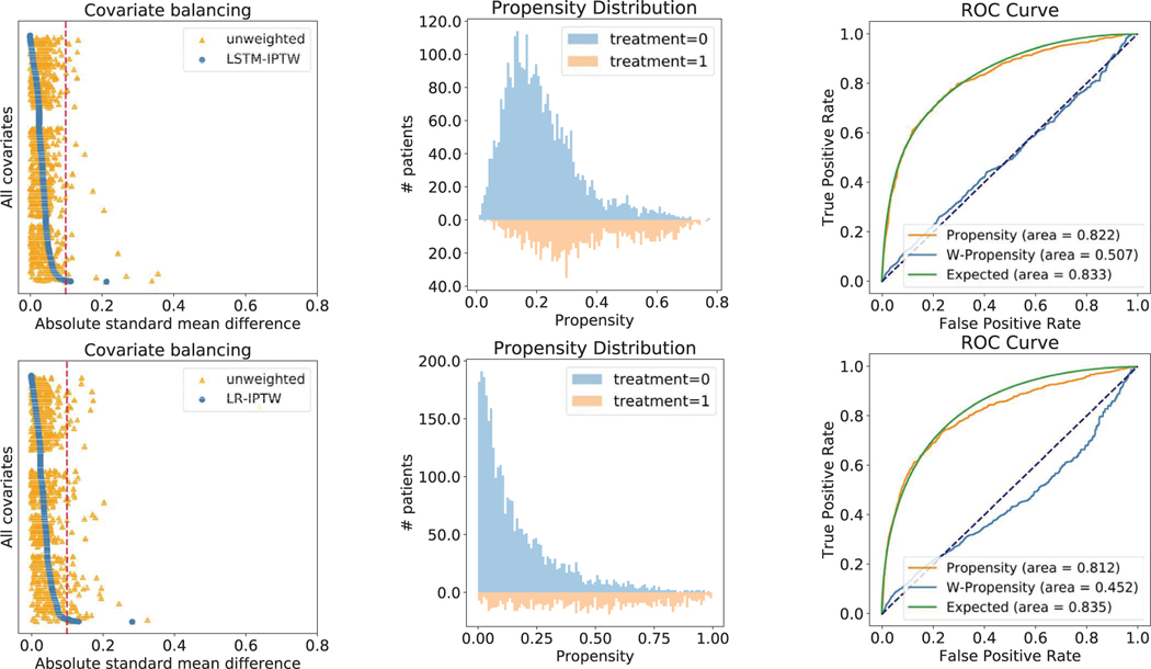
We also developed a base version of our model that uses LR for computing propensity score and treatment effect estimation. A recent study identifying drug repurposing candidates from observational data achieved a good performance on a case study of Parkinson’s disease38. They estimated the propensity scores using LR. Thus, we conduct comparison experiments using the base model (LR-IPTW) and our model (LSTM-IPTW) on the two case drugs above and show the results for diltiazem in Extended Data Fig. 2 (the results for fenofibrate can be found in Supplementary Fig. 1).
As feature balancing is one of the most important evaluation metrics, we first plot the distribution of absolute SMD values computed by LSTM-IPTW and LR-IPTW (Extended Data Fig. 2a,d). In both LSTM- and LR-weighted data, many features exhibit large absolute SMD values (greater than 0.1) in the original data, while most features exhibit low absolute SMD (below 0.1) after re-weighting. Specifically, fewer features exhibit absolute SMD values above 0.1 thresholds after weighting by the LSTM model than weighting by the LR model. This indicates that the data is well balanced by LSTM-IPTW and the estimated ATE from LSTM-IPTW should be more accurate than LR-IPTW. Extended Data Fig. 2b shows the propensity distribution plot over user and non-user cohorts using LSTM-IPTW and LR-IPTW models. We observe that the propensity distribution of LSTM-IPTW is more smooth (that is, the propensities are normally distributed) than the distribution of LR-IPTW. Under the LR-IPTW model, many of the patients in non-user cohorts are predicted to have a propensity of 0. We also evaluated our models using conventional metrics. The receiver operating characteristic (ROC) curve is a standard metric widely used to estimate the performance of prediction models. The area under the ROC curve (AUC) characterizes the accuracy of the prediction results. Extended Data Fig. 2c,f shows the ROC curves for the LSTM-IPTW and LR-IPTW models. The ‘propensity’ curves in the figures are the standard ROC curves of the LSTM and the LR models. By comparing the AUC values of the two models, we see that the LSTM model yields more accurate prediction results than the LR model. With the accurate treatment predictions, the model would generate better weights for balancing and treatment effect estimates in the following tasks. Besides the standard ROC curve, we also show another two curves: the weighted propensity curve and expected curve, which are also leveraged for evaluating causal inference algorithms39. The weighted propensity curve is obtained by re-weighting the standard ROC curve using weights drawn from the propensity model (the same weights applied in covariate balancing and effect estimates). This curve should be very close to the curve that would arise by a random assignment (that is, with an AUC close to 0.5), which indicates our assumption that the weighting can emulate an RCT. From the plots, we find that LSTM-IPTW performs better than LR-IPTW in terms of being closer to 0.5. Compared with the standard propensity ROC curve, the ‘expected’ ROC curve duplicates the population and assigns weights to each individual based on the propensity. In this setting, each patient contributes their propensity to the true positives and (1 − propensity) to the false positives. The standard propensity ROC curve should be close to the expected propensity ROC. We observe that the propensity curve of LSTM-IPTW is much closer to its expected curve than LR-ITPW.
Additional experiments on drug class.
We further consider the drug classes as repurposing candidates to extend the current framework, showing that our repurposing framework can also be applied to drug class level. We group the drugs into sub-classes according to ATC fourth-level (indicating chemical, therapeutic or pharmacological sub-group). Then we regard each drug sub-class as a repurposing candidate and emulate, for each candidate, an RCT to evaluate its treatment effect. The study design remains the same as that for individual drugs except that our studied repurposing candidates are drug classes (ATC fourth level). By applying the selection criteria and study design, we obtain 38 (out of 247) eligible drug classes.
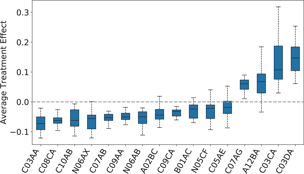
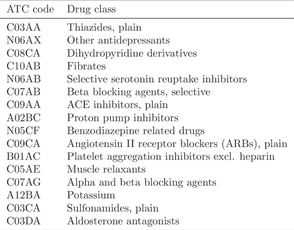
We plot the distribution of estimated ATE values in Extended Data Fig. 3 (the mapping of ATC codes and drug class names is shown in Extended Data Fig. 4). Here, we only show the drug classes with the balanced user and non-user sub-cohorts after re-weighting and statistically significant estimates (adjusted p-value). The results of all 38 drug classes can be found in Supplementary Table 5. All the drug classes are ranked left to right according to the increasing order of estimated ATE values. From the results, we observe that 12 drug classes yield a beneficial effect on disease outcomes among 16 selected significant drug classes.
We also compare the results of drug classes to previous results based on drug ingredients. We observe that most extracted drug classes are consistent with the extracted drug classes in Table 1, while some of them are not. For example, three extracted significant drug ingredients: rosuvastatin, pravastatin and simvastatin, belong to drug class HMG CoA reductase inhibitors (ATC code: C10AA), whereas HMG CoA reductase inhibitors is not a significant drug class. Also, some drug classes (for example, ‘other antidepressants’ and “selective serotonin reuptake inhibitors”) show a beneficial effect with statistical significance in Extended Data Fig. 4, but the drugs that belong to them are not significant nor beneficial to the disease in Table 1.
Drug class offers additional information for drug discovery or drug repurposing tasks. Considering the drug class helps to uncover potential repurposing drug candidates from the drug classes. In future work, we will consider the drug class for drug discovery/repurposing with a more comprehensive analysis.
Additional experiments on drug combinations.
We also evaluate the effect of drug combinations on CAD disease progression. Similar to the experimental setting of individual drugs, we select drug combinations that satisfy the previous cohort definition and criteria (that is, the number of minimum patients in a cohort is no less than 500, window thresholds, persistent prescription and so on). After applying the cohort selection, we obtain seven drug combinations: (1) metoprolol and clopidogrel; (2) metoprolol and atorvastatin; (3) lisinopril and atorvastatin; (4) lisinopril and clopidogrel; (5) metoprolol and lisinopril; (6) clopidogrel and atorvastatin; (7) carvedilol and atorvastatin.
We demonstrate the significant drug combinations in Extended Data Fig. 5 (the full list of drug combinations can be found in Supplementary Table 6). As shown in some drugs are not significant when evaluating their effectiveness at the individual level, while they are significant when combined with others. For example, lisinopril and atorvastatin are not statistically significant as individual treatments, but their drug combination is significant and has a beneficial effect on the outcomes. These results illustrate that considering the synergies of drug combinations provides further interesting findings of potential repurposing.
Comparison with pre-clinical-based methods.
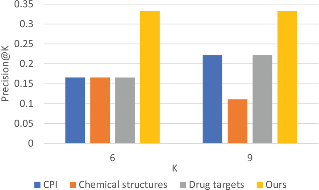
We compare our method with three existing pre-clinical drug repurposing methods40–42 and conduct experiments using CAD as a case study. From the literature43,44, we know that drug chemical structures, protein targets and chemical–protein interactome (CPI) docking are very important for computational pre-clinical drug repurposing methods. We followed the experimental settings of Gottlieb et al.45 to predict drugs for CAD. Specifically, we built an 881-dimensional binary vector for chemical structures following Zhang et al.40 and Liang et al.41. We built a 1,210-dimensional binary vector for protein targets following Zhang et al.40 and Liang et al.41. And we built a 600-dimensional continuous vector for CPI docking scores following Luo et al.42 and Luo et al.4.
For the performance evaluation, we used precision at K (precision@K) as our main evaluation metric to see how many drugs can be validated among the top-ranked candidates. We chose precision@K because given a limited budget, pharmaceutical companies can only evaluate the top-ranked drug candidates instead of all existing on-market drugs. As shown in Extended Data Fig. 6, our method performs better than the other three pre-clinical methods that use CPI docking, drug chemical structures and drug targets as features, respectively. Compared with pre-clinical methods, our method demonstrates two further advantages: (1) fewer translational problems9: we use observational data and emulate the process of RCTs while they only leverage pre-clinical information; (2) it’s more robust: we have strict covariate balancing testing and significance testing that guarantee our results are robust and convincing.
Influence of the model parameters to the results.
We also study the influence of one of our model parameters: adjusted p-value to the results. We slightly relax the threshold for adjusted p-value from 0.05 to 0.15 (ref. 46) and keep the post-weighting unbalanced ratio the same as before. Extended Data Fig. 7 shows the additional repurposing candidates retrieved under this parameter setting (adjusted p-value is less than 0.15 and the post-weighting unbalanced ratio is less than 0.02). As shown in Extended Data Fig. 7, four more drugs are retrieved by our framework. Specifically, (1) metformin, which is the first-line medication for the treatment of type 2 diabetes, and has also been tested for treating CAD in clinical trials47; (2) escitalopram, used to treat major depressive disorder or generalized anxiety disorder48, and some studies have started to explore the drug repurposing opportunity for CAD49; (3) atorvastatin has already been studied in a clinical trial for evaluating its therapeutic effect on CAD50; and (4) losartan has also been included in clinical trials51.
By relaxing the adjusted p-value threshold, we have more drug candidates (for example, metformin and escitalopram) with diverse indications. Our goal is to develop a general computational framework for drug repurposing. For people who want to use our framework, they can easily adjust these parameters according to their preference.
This study can be extended in multiple directions in the future. For this study, we used hypothesized confounders including demographics, co-morbidities and co-prescribed drugs. Some other potential confounders such as time elapsed from the first disease diagnosis to index date and outcome value calculated over the baseline period could be considered to build the model in the future work.
In summary, we demonstrate that the proposed computational drug repurposing framework can successfully identify drug candidates that have a beneficial effect on disease outcomes but aren’t yet indicated for CAD patients. The proposed LSTM-IPTW model performs better at correcting biases and estimating treatment effects than LR-IPTW, and retaining interpretability for recognizing important confounding. We also evaluate the therapeutic effect of drug combinations, drug-class-level candidates on disease outcomes and further explore the potential repurposing opportunity with different model parameters. Besides, we compare our framework with three existing pre-clinical drug repurposing methods and our framework outperforms others.
Methods
In this section, we introduce the study design, which includes definitions of cohorts and study variables. Then we illustrate our deep learning model in detail with three main components.
Study design.
Our framework identifies drug repurposing candidates using MarketScan CAD data to emulate a bulk of corresponding RCTs. Below, we describe the design of the emulated trials and the key components of our framework for CAD drug repurposing.
User and non-user cohorts.
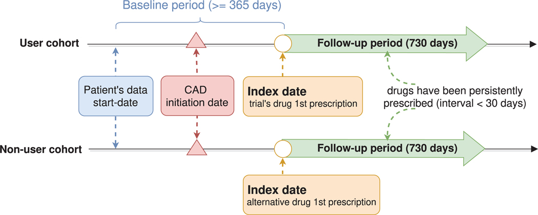
Given the drug tested in the trial, a patient is assigned to the user cohort if the following inclusion criteria are satisfied: (1) the patient has been persistently prescribed the drug (for example, the interval between two prescriptions is less than 30 days); (2) the patient is eligible for trial at the time of the first prsquocription for the drug (in the CAD study, this condition is that the first prescription is after the CAD initiation date); (3) the patient had at least one year’s (365 days) history in the database prior to the first prescription of the drug.
Estimating the effect of a drug requires comparing the user cohort to a control group assigned with alternative drugs. Once the alternative drugs are determined, the non-user cohort is defined by the same inclusion criteria described above— but with respect to the alternative drugs. To avoid overlap between the user and non-user cohorts, the framework further excludes from the non-user cohort any patient prescribed with the trial’s drug. In our study design, alternative drugs are selected randomly from the prescribed ingredients, excluding the trial drug itself. Such a control group directly compares the trial’s drug to drugs of the same therapeutic indication, reducing confounding by indication. We use the term “index date” to refer to the date of the first prescription of the assigned drug, that is, the first time the trial’s drug (respectively, the alternative drug) was prescribed for patients in the user (respectively, non-user) cohort.
Baseline and follow-up periods.
We refer to the time period prior to the index date for which we have information on the patient as the baseline period. We use the baseline period for characterizing the patients prior to the beginning of the treatment with the assigned drug. The follow-up period starts at the index date, that is, at the beginning of the treatment with the trial’s drug in the user cohort, and the control drug in the non-user cohort. The effect of the drug is evaluated during the follow-up period. In the CAD study, the baseline period is at least 365 days, and the follow-up period is 2 years (730 days). Extended Data Fig. 8 demonstrates the definition of user and non-user cohorts.
Outcomes and hypothesized confounders.
The effect of the drug during the follow-up period is defined with respect to various disease outcomes. In this CAD drug repurposing case study, we consulted domain experts to define a set of clinically relevant events linked with CAD as the outcome, for example, heart failure onset (Supplemental Table 2) and stroke onset (Supplemental Table 3). The treatment effect is estimated on these outcomes during the follow-up period (that is, 730 days after the index date). The patient is considered to have the disease outcome if either of them happens in the follow-up period.
Confounders are variables affecting both treatment assignment of patients and an outcome used in the trial, thus creating a ‘backdoor path’ that may hinder the true effect of the drug on the outcome. We consult domain experts to compile a list of hypothesized confounders for the CAD study, including demographics (for example, age at the index date and sex), co-morbidities (for example, indicator per each ICD-9/10 diagnosis class) and co-prescribed drugs. Since confounders affect treatment assignment, they are computed on the baseline period.
Repurposing drug ingredients.
We regard a drug as a repurposing candidate if it satisfies the following conditions: (1) contains an active ingredient (that is, the ingredient directly involved in achieving the mediation objectives); and (2) is persistently prescribed to a large enough number of patients in the disease cohort. Specifically, an ingredient is considered as being used by a patient only if it was prescribed on two or more distinct dates, as least one month apart. And a minimum of 500 patients prescribed a certain ingredient was required. For each repurposing candidate, we can compute the user and non-user cohorts according to the above definition of cohorts. After obtaining the corresponding user and non-user cohorts, we can extract outcomes and hypothesized confounders for each individual patient from the database. Every patient in their sub-cohort is represented by a sequence of events, with each event providing the patient information (that is, co-morbidities, co-prescribed drugs and so on) that corresponds to each visit. The available data within these visits during the baseline period, combined with demographic characteristics (that is, age and gender collected at CAD initiation date) are used as inputs to the model.
Model.
Estimation of ATE.
Our proposed framework evaluates the effect of a certain drug (that is, a trial’s drug) on a clinical outcome with respect to alternative treatments. Let α = 1 denote the treatment corresponding to the trial’s drug, and α = 0 denote the alternative treatments. We define the ATE of a drug on the potential outcome Y as , with denoting the potential expected prevalence of patients who would have experienced an outcome event during a complete follow-up period if all patients in the trial had been assigned with treatment α. The potential outcomes are referred to as counterfactual as only one of these is observed for any given individual. By running RCTs, we can measure the outcomes within user and non-user groups into which individuals are randomly assigned: can be directly estimated as and as . However, in observational data (for example, our MarketScan CAD data), treatment assignment is usually far from random, which may depend on confounders (affecting both treatment assignment and outcome). We need to assign weights to the individuals in each group to avoid the influence of confounders.
In order to control the influence of confounders, we apply IPTW to create a pseudo-population from the original one by assigning a weight to an individual i with treatment α. The weight is defined as the inverse of the conditional probability (or propensity score) that an individual is treated with α given the confounding values. One common issue with IPTW is that individuals with a propensity score very close to 0 will end up with an extremely high weight, potentially making the weighted estimator unstable. We address this problem by adopting an alternative weighting function called standardized IPTW25, which uses the marginal probability of treatment instead of 1 in the weight numerator.
Logistic regression is the most popular method in statistics for estimating the propensity score52. In longitudinal observational data, those observational covariates are not a set of static feature vectors (one for each patient), but irregularly sampled time series (recording diagnoses, medications and so on at each timestamp). Thus, logistic regression is not ideal for effectively modelling longitudinal observational data.
Model for propensity score weighting.
The schematic view of our model is shown in Fig. 2, which consists of three main components: an embedding module, a recurrent neural network and a prediction module. Briefly, the model estimates the propensity score by first transforming the input features using an embedding layer. These embedded features are then fed into LSTM, the output of which at every time point is aggregated through an attention layer for automatically focusing on important time points. The aggregated features are fed into a prediction module that provides the probability of receiving treatment. Each of these is discussed below in detail.
Embedding module.
The embedding module is to convert the initial high-dimensional and sparse input features into a lower-dimensional and continuous data representation, which is beneficial to the following prediction task. As shown in Fig. 2, the input features consist of three components: diagnosis, prescription and demographic information (age and gender). The diagnosis codes for each patient at each timestamp can be denoted as , and prescription can be denoted as . Here, dt and pt are both one dimensional binary vectors with the size of diagnosis code dictionary (r) and prescription code dictionary (s), respectively. For each element in the vector, the value in the j-th column indicates that code j is documented in the t-th visit. We use two linear embedding modules to represent diagnosis and prescription respectively. That is, we define , , where denotes the embedding of the input vector , m is the size of the diagnosis embedding dimension, and is the embedding matrix. denotes the embedding of the input vector , n is the size of the diagnosis embedding dimension, and is the embedding matrix. The age is normalized into a range of [0, 1] using min–max normalization and the gender is represented as a binary vector. Having the embedded vectors of patients, we input them to LSTM.
Recurrent neural network and attention mechanism.
LSTM15, which is a kind of recurrent neural network equipped with memory cells, can better model the temporality of observational data. A common LSTM unit contains a cell, an input gate, an output gate and a forget gate. The cell can remember values over irregular time intervals and the three gates moderate the flow of information into and out of the cell. The inputs to the LSTM are embedded confounding vectors from the embedding module and the output of which is the patient’s latent health status at the time of visit. We use two LSTMs, LSTMα and LSTMβ to separately model diagnosis and prescription codes of patients.
| (3) |
where , are hidden state vectors at t-th visit, and u and v denote the size of hidden layer of LSTMα and LSTMβ. Then those patient hidden states are aggregated through two separate attention layers for automatically focusing on important visits.
| (4) |
where and are the parameters to learn. Using the generated attention weights for diagnosis and prescription, we obtain the aggregated vectors and as defined in equation (4). Then we combine cα, cβ with vectorized age and gender to predict the probability of receiving a treatment (propensity score).
Prediction module.
The aggregated patient states from attention layer cα, cβ, combined with the demographic features cdemo, are passed through a fully connected neural network to predict the probability of receiving a treatment as follows,
| (5) |
where are the model parameters. We use cross-entropy to calculate the prediction loss as follows,
| (6) |
where yi is the ground truth of observed treatment for patient i.
Experiment settings.
The model is implemented and trained with Python 3.6 and PyTorch 1.4 (https://pytorch.org/), on a high-performance computing cluster with four NVIDIA TITAN RTX 6000 GPUs. For each drug candidate, we train a model using the adaptive moment estimation (Adam) algorithm with a batch size of 50 subjects and a learning rate of 0.001. We run each model for 50 iterations for computing p-values and confidence intervals. We randomly split the input data into training, validation and test sets with a ratio of 70:10:20. The information from a given patient is only present in one set. The training set is to train the proposed models. The validation set is used to improve the models and select the best model hyperparameters.
Extended Data
Extended Data Fig. 1 |. CAD cohorts characteristics.
a, The patients’ distribution of total time in the database. b, The patient’s distribution of time before/after CAD initiation date. c, The growth of the number of patients developing outcomes after CAD initiation date. d, The gender distribution with age at CAD initiation date.
Extended Data Fig. 2 |. Performance comparison of LSTM-IPTW and LR-IPTW using drug candidate: diltiazem (with known CAD indication).
The three figures on the top are results obtained from LSTM-IPTW, while the figures on the bottom are from LR-IPTW. a, and (d) The absolute SMD of each covariate in the original data (orange triangles) and in the weighted data (blue circles). b, and (e) The distribution of estimated propensity scores over user (orange area) and non-user (blue area) cohorts. c, and (f) The ROC curves for the propensity model (orange), expected value (green) and weighted propensity (blue).
Extended Data Fig. 3 |. Distribution of estimated ATE of drug classes on defined outcomes across the 50 bootstrap samples.
All these showing drug classes satisfy two conditions: adjusted p-value less than 0.05 and post unbalanced ratio less than 2%. Within the boxplot, the central line denotes the median, and the bottom and the top edges denote the 25th(Q1) and 75th(Q3) and percentiles respectively. The whiskers extend to 1.5 times the interquartile range.
Extended Data Fig. 4 |. The list of significant drug classes.
The drug classes are denoted using ATC code and corresponding names.
Extended Data Fig. 5 |. The estimated treatment effects for CAD over balanced and statistically significant drug combinations.
The drug combinations are ranked by the estimated ATE values.
Extended Data Fig. 6 |. Performance comparison of proposed method and three pre-clinical methods evaluated by Precision@K.
The values of K are selected from {6, 9}.
Extended Data Fig. 7 |. Retrieved additional repurposing candidates under different thresholds’ setting.
The adjusted p-value is changed to 0.15 and the post unbalanced ratio remains the same as previous setting (less than 2%).
Extended Data Fig. 8 |. The definition of user and non-user cohorts.
Index date refers to the first prescription of the trial’s drug (user cohort) or the alternative drug (non-user cohort). The time period before the index date is the baseline period, and the time after the index date is the follow-up period. The patient covariates are collected during the baseline period and the treatment effects are evaluated at the follow-up period.
Supplementary Material
Acknowledgements
This work was funded in part by the National Center for Advancing Translational Research of the National Institutes of Health under award number CTSA Grant UL1TR002733. The content is solely the responsibility of the authors and does not necessarily represent the official views of the National Institutes of Health.
Footnotes
Competing interests
The authors declare no competing interests.
Additional information
Extended data is available for this paper at https://doi.org/10.1038/s42256-020-00276-w.
Supplementary information is available for this paper at https://doi.org/10.1038/s42256-020-00276-w.
Peer review information Nature Machine Intelligence thanks Daniel Merk and the other, anonymous, reviewer(s) for their contribution to the peer review of this work.
Code availability
The source code for this paper can be downloaded from the Github repository at https://github.com/ruoqi-liu/DeepIPWor the Zenodo repository at https://doi.org/10.5281/zenodo.4079391.
Data availability
The data we use is MarketScan Commercial Claims and Encounters (CCAE, more than 100 million patients, from 2012 to 2017) The details of source data structure and prepossessed input data demo are available at the Github repository https://github.com/ruoqi-liu/DeepIPW. Access to the MarketScan data analysed in this manuscript is provided by the Ohio State University. The dataset is available from IBM at https://www.ibm.com/products/marketscan-research-databases.
References
- 1.Langedijk J, Mantel-Teeuwisse AK, Slijkerman DS & Schutjens M-HD Drug repositioning and repurposing: terminology and definitions in literature. Drug Discov. Today 20, 1027–1034 (2015). [DOI] [PubMed] [Google Scholar]
- 2.Ashburn TT & Thor KB Drug repositioning: identifying and developing new uses for existing drugs. Nat. Rev. Drug Discov 3, 673–683 (2004). [DOI] [PubMed] [Google Scholar]
- 3.Pushpakom S. et al. Drug repurposing: progress, challenges and recommendations. Nat. Rev. Drug Discov 18, 41–58 (2019). [DOI] [PubMed] [Google Scholar]
- 4.Luo H. et al. DPDR-CPI, a server that predicts drug positioning and drug repositioning via chemical-protein interactome. Sci. Rep 6, 35996 (2016). [DOI] [PMC free article] [PubMed] [Google Scholar]
- 5.Dakshanamurthy S. et al. Predicting new indications for approved drugs using a proteochemometric method. J. Med. Chem 55, 6832–6848 (2012). [DOI] [PMC free article] [PubMed] [Google Scholar]
- 6.Sanseau P. et al. Use of genome-wide association studies for drug repositioning. Nat. Biotechnol 30, 317–320 (2012). [DOI] [PubMed] [Google Scholar]
- 7.Iorio F. et al. Discovery of drug mode of action and drug repositioning from transcriptional responses. Proc. Natl Acad. Sci USA 107, 14621–14626 (2010). [DOI] [PMC free article] [PubMed] [Google Scholar]
- 8.Sirota M. et al. Discovery and preclinical validation of drug indications using compendia of public gene expression data. Sci. Transl. Med 3, 96ra77 (2011). [DOI] [PMC free article] [PubMed] [Google Scholar]
- 9.Buchan NS et al. The role of translational bioinformatics in drug discovery. Drug Discov. Today 16, 426–434 (2011). [DOI] [PubMed] [Google Scholar]
- 10.Sherman RE et al. Real-world evidence—what is it and what can it tell us. N. Engl. J. Med 375, 2293–2297 (2016). [DOI] [PubMed] [Google Scholar]
- 11.Cheng F. et al. Network-based approach to prediction and population-based validation of in silico drug repurposing. Nat. Commun 9, 2691 (2018). [DOI] [PMC free article] [PubMed] [Google Scholar]
- 12.Xu H. et al. Validating drug repurposing signals using electronic health records: a case study of metformin associated with reduced cancer mortality. J. Am. Med. Inform. Assoc 22, 179–191 (2014). [DOI] [PMC free article] [PubMed] [Google Scholar]
- 13.Hernán MA & Robins JM Using big data to emulate a target trial when a randomized trial is not available. Am. J. Epidemiol 183, 758–764 (2016). [DOI] [PMC free article] [PubMed] [Google Scholar]
- 14.D’Agostino RB Estimating treatment effects using observational data. JAMA 297, 314–316 (2007). [DOI] [PubMed] [Google Scholar]
- 15.Hochreiter S. & Schmidhuber J. Long short-term memory. Neural Comput. 9, 1735–1780 (1997). [DOI] [PubMed] [Google Scholar]
- 16.Hirano K, Imbens GW & Ridder G. Efficient estimation of average treatment effects using the estimated propensity score. Econometrica 71, 1161–1189 (2003). [Google Scholar]
- 17.MarketScan Research Databases. IBM https://www.ibm.com/products/marketscan-research-databases (2020).
- 18.Commercial Claims and Encounters: Medicare Supplemental https://theclearcenter.org/wp-content/uploads/2020/01/IBM-MarketScan-User-Guide.pdf (Truven Health Analytics, 2016). [Google Scholar]
- 19.Classification of diseases, functioning, and disability. Centers for Disease Control and Prevention; https://www.cdc.gov/nchs/icd/index.htm (2019). [Google Scholar]
- 20.The Observational Health Data Sciences and Informatics (OHDSI). https://ohdsi.org/ (2019).
- 21.Causes of heart failure. American Heart Association https://www.heart.org/en/health-topics/heart-failure/causes-and-risks-for-heart-failure/causes-of-heart-failure (2017).
- 22.Gheorghiade M. & Bonow RO Chronic heart failure in the united states: a manifestation of coronary artery disease. Circulation 97, 282–289 (1998). [DOI] [PubMed] [Google Scholar]
- 23.Conditions that increase risk for stroke. Centers for Disease Control and Prevention https://www.cdc.gov/stroke/conditions.htm (2018).
- 24.Coronary artery disease. Heart and Stroke Foundation of Canada https://www.heartandstroke.ca/heart/conditions/coronary-artery-disease (2019).
- 25.Austin PC An introduction to propensity score methods for reducing the effects of confounding in observational studies. Multivariate Behav. Res 46, 399–424 (2011). [DOI] [PMC free article] [PubMed] [Google Scholar]
- 26.Efron B. & Tibshirani R. Bootstrap methods for standard errors, confidence intervals, and other measures of statistical accuracy. Stat. Sci 1, 54–75 (1986). [Google Scholar]
- 27.Benjamini Y. & Hochberg Y. Controlling the false discovery rate: a practical and powerful approach to multiple testing. J. R. Stat. Soc. B 57, 289–300 (1995). [Google Scholar]
- 28.Kuhn M, Campillos M, Letunic LJ & Bork P. A side effect resource to capture phenotypic effects of drugs. Mol. Syst. Biol 6, 343 (2010). [DOI] [PMC free article] [PubMed] [Google Scholar]
- 29.Wishart DS et al. Drugbank 5.0: a major update to the drugbank database for 2018. Nucleic Acids Res. 46, D1074–D1082 (2018). [DOI] [PMC free article] [PubMed] [Google Scholar]
- 30.Fisher ML et al. Beneficial effects of metoprolol in heart failure associated with coronary artery disease: a randomized trial. J. Am. Coll. Cardiol 23, 943–950 (1994). [DOI] [PubMed] [Google Scholar]
- 31.Wong TY, Simó R. & Mitchell P. Fenofibrate – a potential systemic treatment for diabetic retinopathy?. Am. J. Ophthalmol 154, 6–12 (2012). [DOI] [PubMed] [Google Scholar]
- 32.Hydrochlorothiazide. drugs.com https://www.drugs.com/monograph/hydrochlorothiazide.html (2019).
- 33.Pepine CJ et al. A calcium antagonist vs a non–calcium antagonist hypertension treatment strategy for patients with coronary artery disease: the international verapamil-trandolapril study (invest): a randomized controlled trial. JAMA 290, 2805–2816 (2003). [DOI] [PubMed] [Google Scholar]
- 34.Jukema JW et al. Effects of lipid lowering by pravastatin on progression and regression of coronary artery disease in symptomatic men with normal to moderately elevated serum cholesterol levels: the regression growth evaluation statin study (regress). Circulation 91, 2528–2540 (1995). [DOI] [PubMed] [Google Scholar]
- 35.Kjekshus J, Pedersen TR, Olsson AG, Færgeman O. & Pyörälä K. The effects of simvastatin on the incidence of heart failure in patients with coronary heart disease. J. Card. Fail 3, 249–254 (1997). [DOI] [PubMed] [Google Scholar]
- 36.Higuchi T, Abletshauser C, Nekolla SG, Schwaiger M. & Bengel FM Effect of the angiotensin receptor blocker valsartan on coronary microvascular flow reserve in moderately hypertensive patients with stable coronary artery disease. Microcirculation 14, 805–812 (2007). [DOI] [PubMed] [Google Scholar]
- 37.Diltiazem. SIDER http://sideeffects.embl.de/drugs/3075/ (2019).
- 38.Ozery-Flato M, Goldschmidt Y, Shaham O, Ravid S. & Yanover C. Framework for identifying drug repurposing candidates from observational healthcare data. Preprint at medRxiv 10.1101/2020.01.28.20018366 (2020). [DOI] [PMC free article] [PubMed]
- 39.Shimoni Y. et al. An evaluation toolkit to guide model selection and cohort definition in causal inference. Preprint at https://arxiv.org/abs/1906.00442 (2019).
- 40.Zhang P, Wang F, Hu J. & Sorrentino R. Exploring the relationship between drug side-effects and therapeutic indications. In AMIA Annual Symposium Proceedings 2013 1568–1577 (American Medical Informatics Association, 2013). [PMC free article] [PubMed] [Google Scholar]
- 41.Liang X. et al. LRSSL: predict and interpret drug–disease associations based on data integration using sparse subspace learning. Bioinformatics 33, 1187–1196 (2017). [DOI] [PubMed] [Google Scholar]
- 42.Luo H. et al. DRAR-CPI: a server for identifying drug repositioning potential and adverse drug reactions via the chemical–protein interactome. Nucleic Acids Res. 39, W492–W498 (2011). [DOI] [PMC free article] [PubMed] [Google Scholar]
- 43.Dudley JT, Deshpande T. & Butte AJ Exploiting drug–disease relationships for computational drug repositioning. Brief. Bioinform 12, 303–311 (2011). [DOI] [PMC free article] [PubMed] [Google Scholar]
- 44.Jarada TN, Rokne JG & Alhajj R. A review of computational drug repositioning: strategies, approaches, opportunities, challenges, and directions. J. Cheminf 12, 46 (2020). [DOI] [PMC free article] [PubMed] [Google Scholar]
- 45.Gottlieb A, Stein GY, Ruppin E. & Sharan R. PREDICT: a method for inferring novel drug indications with application to personalized medicine. Mol. Syst. Biol 7, 496 (2011). [DOI] [PMC free article] [PubMed] [Google Scholar]
- 46.Rubinstein LV et al. Design issues of randomized phase II trials and a proposal for phase ii screening trials. J. Clin. Oncol 23, 7199–7206 (2005). [DOI] [PubMed] [Google Scholar]
- 47.Metformin to reduce heart failure after myocardial infarction (gips-iii). clinicaltrials.gov https://clinicaltrials.gov/ct2/show/study/NCT01217307?term=metformin&cond=Coronary+Artery+Disease&phase=12&draw=2&rank=2 (2018).
- 48.Escitalopram oxalate. drugs.com https://www.drugs.com/monograph/escitalopram-oxalate.html (2020).
- 49.Responses of myocardial ischemia to escitalopram treatment (remit). clinicaltrials.gov https://clinicaltrials.gov/ct2/show/NCT00574847?term=escitalopram&cond=Coronary+Artery+Disease&draw=2&rank=1 (2015). [DOI] [PMC free article] [PubMed]
- 50.Effect of atorvastatin on fractional flow reserve in coronary artery disease (forte). clinicaltrials.gov https://clinicaltrials.gov/ct2/show/NCT01946815?term=atorvastatin&cond=Coronary+Artery+Disease&phase=12&draw=2&rank=1 (2018).
- 51.Dahlöf B. et al. Cardiovascular morbidity and mortality in the losartan intervention for endpoint reduction in hypertension study (life): a randomised trial against atenolol. Lancet 359, 995–1003 (2002). [DOI] [PubMed] [Google Scholar]
- 52.D’Agostino RB Jr Propensity score methods for bias reduction in the comparison of a treatment to a non-randomized control group. Stat. Med 17, 2265–2281 (1998). [DOI] [PubMed] [Google Scholar]
Associated Data
This section collects any data citations, data availability statements, or supplementary materials included in this article.
Supplementary Materials
Data Availability Statement
The data we use is MarketScan Commercial Claims and Encounters (CCAE, more than 100 million patients, from 2012 to 2017) The details of source data structure and prepossessed input data demo are available at the Github repository https://github.com/ruoqi-liu/DeepIPW. Access to the MarketScan data analysed in this manuscript is provided by the Ohio State University. The dataset is available from IBM at https://www.ibm.com/products/marketscan-research-databases.


