Viable closed-loop supply chain network by considering robustness and risk as a circular economy

Abstract

The viable closed-loop supply chain network (VCLSCND) is a new concept that integrates sustainability, resiliency, and agility into a circular economy. We suggest a hybrid robust stochastic optimization by minimizing the weighted expected, maximum, and entropic value at risk (EVaR) of the cost function for this problem. This form considers robustness against demand disruption. Finally, CLSC components are located, and quantity flows are determined in the automotive industry. The results show that the VCLSCND cost is less than not considering viability and has a − 0.44% gap. We analyze essential parameters. By increasing the conservative coefficient, confidence level, and the scale of the main model, decreasing the allowed maximum energy, the cost function, time solution, and energy consumption grow. We suggested applying the Fix-and-Optimize algorithm for producing an upper bound for large-scale. As can be seen, the gap between this algorithm and the main problem for cost, energy, and time solution is approximately 6.10%, − 8.28%, and 75.01%.

Introduction

The closed-loop supply chain (CLSC) is a complete SC that considers sustainability and a circular economy (Difrancesco & Huchzermeier 2016; Rafigh et al., 2021). Paying more attention to returned products does not allow to release of returned products to environments. Therefore, a CLSC network design (CLSCND) that integrates sustainability, resiliency, and agility is the discussion of researchers. The viable CLSCND (VCLSCND) concept combines sustainability, resiliency, and agility in CLSCND (Ivanov & Dolgui 2020) (Fig. 1). We try to improve organizational, informational, technological, financial, and process-functional structure in VCLSCND. We can add backup suppliers, flexible capacity and sourcing, and increase inventory and capacity to fortify resiliency.

Fig. 1.

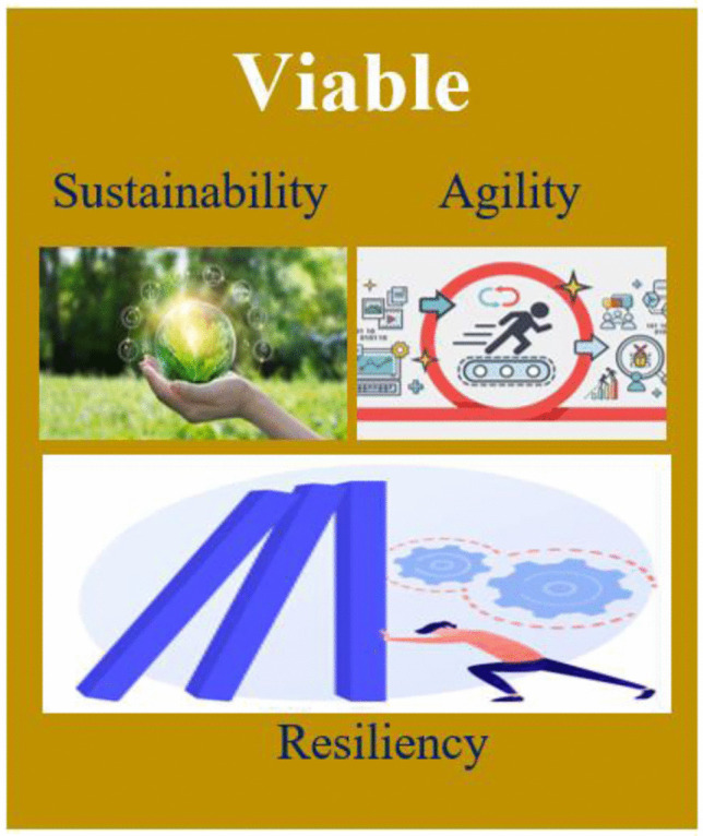
Concept of viability in network design

Moreover, requirements of the environment, energy consumption, and social welfare can be seen in the sustainability subject (Mehrbakhsh & Ghezavati 2020). Eventually, delivery on time with a responsive SC is needed as an agile supply chain. Using novel technology like blockchain and Internet-of-Thing (IoT), 3D printing aims as an agile tool in VCLSCND (Lotfi et al. 2021e). We should design a VCLSCND that enables us to cope with uncertainty and robust disruption.

This subject has been raised, originating from decision-making challenges due to the COVID19 outbreak and global pandemic. It makes disturbance for demand and changes sustainability among social welfare like occupation and employment. We need CLSCND to be resilient against these fluctuations (Simchi-Levi & Simchi-Levi 2020). The advantage of this network design is adapting to all situations and having flexibility (Paul & Chowdhury 2020). In addition, this way of thinking guarantees that move toward leanness and agility, and their combination is Leagility. Therefore, researchers need a network that maintains itself and survives in a changing environment over a long period by redesigning the structures and replanning economic performance with long-term impacts (Ivanov 2020; Ivanov & Dolgui 2020).

If we want to move to globalization and have global SC, it is inevitable to redesign SC in the form of viable until improving the performance of SCND (Lotfi et al., 2021a; Zare Mehrjerdi & Lotfi 2019). The further we go, changing the society is fast; as a result, all SCND should transform to VCLSCND as soon as possible until they can stand (Hosseini et al. 2019).

We need to consider all requirements of resiliency that fortify by the flexible facility and increase suppliers to resilience in complex situations. Shocks like COVID-19, natural disasters, unnatural disasters, and risks may disturb CLSC (Srivastava & Rogers 2021). We must always be ready and flexible with various products and services to tackle demand fluctuation. Therefore, if we run a VCLSCND considering risk and robustness, we can establish a global SC with the ability to face any problems.

The innovation and contribution are as follows:

1. A viable CLSCND (VCLSCND) as a circular economy,

2. Integrating sustainability, resiliency, and agility in VCLSCND,

3. Considering risks and robustness in VCLSCND.

We prepared this research as follows. In the “Related work about SCND” section, we survey the literature review and related work and suggest gap research in the scope of SCND. The “Problem statement” section determines the VCLSCND mathematical, linearization, and solution approach. In the “Results and discussion” section, the results and sensitivity analysis are explained. In the “Managerial insights and practical implications” section, the managerial insights are presented. In the “Conclusions and outlook” section, the conclusion and outlook are drawn.

Survey on related work

In this section, we survey related work about type of SCND. The researchers develop many contributions to this issue. However, this issue has many research gaps; integrating resiliency, sustainability, and agility is not defined.

Sustainable SCND

Santander et al. (2020) suggested the first formulation for CLSCND of distributed plastic recycling for 3D printing. They determined economic and environmental objectives. They utilized GAMS solver for optimizing. Pourmehdi et al. (2020) designed a SCLSCND considering production technology for the steel industry. They utilized a scenario-based multi-objective to show uncertainty. Their objectives are optimizing total profit, energy, and water consumption, CO₂ emission, and job opportunity. They embedded a fuzzy goal programming approach to solve the model.

Nayeri et al. (2020) developed a SCLSCND. They integrated strategic and tactical decisions in their model and optimized financial, environmental, and social impacts by a multi-objective fuzzy robust optimization approach. Their case study was a water tank.

Diabat and Jebali (2021) presented a CLSCND for durable products with take-back legislation. Each returned product had three recovery options based on its quality, economic value, and environmental impact. Their case study was washing machines and tumble dryers. They found that the recovery of used products is not profitable for CLSCND.

Salehi-Amiri et al. (2021a, b) designed a SCLSCND based on a triple bottom line approach. Their model indicates economic, environmental, and social impacts (created job opportunities). They utilized a hybrid Imperialist Competitive Algorithms (ICA) and variable neighborhood search as a solution approach.

In other works of Salehi-Amiri et al. (2021b)they survey a SCLSCND in the agriculture industry. They suggested a bi-objective model, including cost and job creation in the avocado industry. They found that decreasing demand, make to increases cost and improve employment efficiency.

Soleimani et al. (2021) suggested a SCLSCND by inspiring from circular economy paradigm. They established a tradeoff between economic and environmental sustainability. They designed a green CLSCND to minimize cost and carbon emission. They utilized Augmented Weighted Tchebycheff (AWT) and ε-constraint as a solution approach.

Tehrani and Gupta (2021) investigated a sustainable green CLSC with various capacity levels. They applied the proposed CLSCND in the tire industry. They used a fuzzy robust stochastic optimization approach (FRSO) for uncertainty parameters and considered recovery options.

Resilient and sustainable SCND

Zare Mehrjerdi and Lotfi (2019) designed a resilient and sustainable CLSCND (RSCLSCND) by considering resilience, robustness, sustainability, and risk aversion. They used a hybrid two-stage stochastic robust optimization by adding conditional VaR (CVaR). Four objectives include minimizing the costs, CO₂ emission, energy, and maximizing employment. They applied Lp-metric to draw the Pareto front. They employed fix-and-optimize and a constraint relaxation to generate the upper and lower bounds.

In other work, Lotfi et al. (2021d) suggested and developed two algorithms for solving a RSCLSCND. They proposed a constraint relaxation and worst-case method as a hybrid model that contains robust stochastic optimization with risk.

Moreover, Lotfi et al. (2021a) contributed a new RSSCND by adding renewable energy for the first time. This RSSCND applied renewable energy to prepare the energy for SCND. They applied a fix-and-optimize algorithm to minimize cost and determine a large-scale problem’s upper bound.

Mehrjerdi and Shafiee (2021) presented a RSCLSCND with information sharing and multiple sourcing as resilience strategies. They utilized multiple sourcing and information sharing for resiliency strategy. They used total cost, pollution, energy consumption, and job creation as objective functions. They embedded the Augmented ε-constraint (AUGMECON2) method as a solution approach.

Fazli-Khalaf et al. (2021) developed a sustainable and resilient tire CLSCND. They suggested four objectives function: minimizing the total costs, maximizing the coverage of customers’ demand, maximizing the reliability of facilities, and minimizing CO2 emissions. A Fuzzy Possibilistic Flexible Programming (FPFP) method is contributed to coping with uncertainty.

Yavari and Ajalli (2021) investigated a resiliency strategy for a green-resilient SCND with a supplier coalition. They compared coalition strategy with single-source and multi-source retailers. The green-resilient model reduced costs by 14% compared to the non-resilient model.

Nayeri et al. (2021) contributed to a sustainable SCND by considering a resilience and responsiveness strategy. The model aims to minimize the total cost and environmental impact by maximizing the social effects. An improved version of FRSO is utilized to tackle uncertainty. They used meta-goal programming to optimize the model. A case study in the water heater industry is suggested to show the model’s performance.

Research gap

We arranged the survey of related work in Table 1. As can be seen, we want to design VCLSCND that is not developed yet. The contribution of this research is as follows:

1. We suggest VCLSCND through sustainability constraints, resilience strategy (flexible capacity), and agility.

2. Finally, we proposed robust stochastic optimization as an uncertainty method by defining a new form that includes a hybrid EVaR, minimax, as a risk objective function.

Table 1.

Survey on related work

Ref	Type of SCND	Viable			Method	Risk criteria	Uncertainty	Case study
		Resilience	Sustainable	Agile
Zare Mehrjerdi and Lotfi, 2019)	RCLSCNDR	✓	✓	-	MILP + Lp-metric, Fix-and-opt	CVaR	Robust scenario-based	Automotive
Pourmehdi et al. (2020)	SCLSCND	-	✓	-	MILP	-	Scenario-based	Steel
Nayeri et al. (2020)	SCLSCND	-	✓	-	MILP	-	FRO	Water tank
Santander et al. (2020)	SCLSCND	-	✓	-	MILP	-	-	3D printing
Salehi-Amiri, et al. (2021a, b)	SCLSCND	-	✓	-	MILP + 3 Meta-heuristic	-	-	Numerical example (NE)
Diabat and Jebali (2021)	SCLSCND	-	✓	-	MILP	-	-	Washing machines and tumble dryers
Lotfi et al. (2021c)	RSCLSCNDR	✓	✓	-	MILP	CVaR	Robust scenario-based	Automotive
Lotfi et al. (2021b)	RSSCNDRE	✓	✓	-	MILP	-	Robust scenario-based	NE
Lotfi et al. (2021f)	RSCLSCNDR	✓	✓	-	MILP	CVaR, EVaR and Minimax	Robust scenario-based	Automotive
Mehrjerdi and Shafiee (2021)	RCLSCND	✓	✓	-	MILP + AUGMECON2	-	Scenario-based	Tire
Salehi-Amiri et al. (2021b)	SCLSCND	-	✓	-	MILP	-	-	Avocado
Soleimani et al. (2021)	SCLSCND	-	✓	-	MILP + AWT	-	Robust optimization	NE
Fazli-Khalaf et al. (2021)	RSCLSCND	✓	✓	-	MILP	-	FPFP	Tire
Yavari and Ajalli (2021)	RSSCND	✓	✓	-	MILP	-	-	Dairy
Nayeri et al. (2021)	RSCND	✓	✓	✓	MILP	-	FRSO	Water heater industry
Tehrani and Gupta (2021)	SCLSCND	-	✓	-	MILP	-	FRSO	Tire
Fu et al. (2021)	Couple CLSCND	-	✓	-	MILP	-	-	NE
Tirkolaee et al. (2022a, b)	CLSCND	-	✓	-	MILP + Pareto-based algorithms	-	-	NE
Salehi-Amiri et al. (2022)	CLSCND	-	✓	-	MILP	-	-	Avocado industry
Kim and Do Chung (2022)	CLSCND	-	✓	-	MILP	-	-	NE
This research	VCLSCND	✓	✓	✓	MILP	EVaR minimax	Robust scenario-based	Automotive

MILP, mixed-integer linear programming

In comparison between our methodology and related work, we cannot see VCLSND in the literature review. There are only (Lotfi et al., 2021d; f) and (Fazli-Khalaf et al. 2021) that are not considered agility and risk completely. In addition, we propose two types of resilience strategy (the flexible capacity facility, multi-resource) that is not applied in the previous study.

Eventually, this model presents a resilience strategy through the flexible capacity facility, multi-resource (supplier and distribution), sustainable approach through presenting energy consumption constraints, and agile method by offering satisfaction demand. Also, we propose a new form of cost objective function for robustness against demand disruption. This form includes minimizing the weighted expected, maximum, and EVaR cost function that was not considered in the previous study.

Problem statement

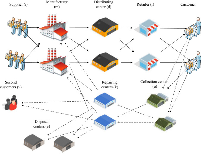
In this research, we propose VCLSCND that considers resiliency, sustainability, and agility in CLSCND, and the previous section shows a lack of research. This study has customers, retailers, distributing centers, manufacturers, suppliers, recovery centers, repair centers, disposal centers, and second customers (Fig. 2). We applied a new form of robust stochastic optimization by minimizing the weighted expected, maximum, and EVaR cost function. We suggest this form of robustness and risk-averse against demand fluctuation in a circular economy. We apply viable policies, including resilience strategy, sustainable strategy, and agile approach.

Fig. 2.

VCLSCND with considering robustness and risk

Eventually, we suggested VCLSCND based on this scope:

1. Resilience strategy: we present resilience strategy through the flexible capacity facility, multi-resource (supplier and distribution),

2. Sustainable strategy: we present energy consumption constraints,

3. Agile approach: we offer satisfaction demand.

Therefore, this assumption is needed as follows:

Assumption

• All demands should be satisfied, and the shortage is not allowed (agility),

• Flow and capacity constraints in forwarding and backward SC are established (agility),

• Sustainability constraint includes energy consumption are determined (sustainability),

• Flexible capacity based on scenarios for each facility is a resilience strategy (resiliency),

• Robust stochastic optimization is applied to cope with demand fluctuation (resiliency) (Ivanov 2020; Lotfi et al. 2021d).

Notation list.

Indices:

$i$	Index of suppliers $i\in I=\{1,2,...,i\},$
$m$	Index of producer (manufacturers)$m\in M=\{1,2,...,\overline{m}\},$
$d$	Index of Distributing Centers (DC)$d\in D=\{1,2,...,\overline{d}\},$
$r$	Index of retailers $r\in R=\{1,2,...,\overline{r}\},$
$u$	Index of collection centers $u\in U=\{1,2,...,\overline{u}\},$
$k$	Index of repairing centers $k\in K=\{1,2,...,\overline{k}\},$
$e$	Index of disposal centers $e\in E=\{1,2,...,\overline{e}\},$
$v$	Index of second customers $v\in V=\{1,2,...,\overline{v}\},$
$p$	Index of commodity (products)$p\in P=\{1,2,...,\overline{p}\},$
$t$	Index of time period $t\in T=\{1,2,...,\overline{t}\},$
$s$	Index of scenario $s\in S=\{1,2,...,\overline{s}\}.$

Parameters

		Value for case study	Unit
$d{d}_{\mathit{rpts}}$	Demand in retailer $r$ for commodity $p$ in period $t$ under scenario $s,$	(s-1).40 + U(20,60)	Number
Costs:
$f{i}_i$	Activation cost for supplier $i,$	U(1,2).1000	Thousand Dollars (TDollar)
$f{m}_m$	Activation cost for manufacture	U(4,5).10000	TDollar
$f{d}_d$	Activation cost for DC $d,$	U(3,4).1000	TDollar
$f{r}_r$	Activation cost for retailer $r,$	U(1,2).1000	TDollar
$f{u}_u$	Activation cost for collection centers $u$,	U(2,3).1000	TDollar
$f{k}_k$	Activation cost for repairing centers $k$,	U(2,3).1000	TDollar
$f{e}_e$	Activation cost for disposal centers $e$,	U(1,2).1000	TDollar
$vi{m}_{\mathit{impts}}$	Variable cost for shipment from supplier $i$ to manufacture $m$ for commodity $p$ in period $t$ under scenario $s,$	U(3,4)/1000	TDollar
$vm{d}_{\mathit{mdpts}}$	Variable cost for shipment from manufacturer $m$ to DC $d$ for commodity $p$ in period $t$ under scenario $s,$	U(3,4)/1000	TDollar
$vd{r}_{\mathit{drpts}}$	Variable cost for shipment from DC $d$ to retailer $r$ for commodity $p$ in period $t$ under scenario $s,$	U(3,4)/1000	TDollar
$vr{u}_{\mathit{rupts}}$	Variable cost for shipment from retailer $r$ to collection centers $u$ for commodity $p$ in period $t$ under scenario $s,$	U(3,4)/1000	TDollar
$vu{k}_{\mathit{ukpts}}$	Variable cost for shipment from collection centers $u$ to repairing centers $k$ for commodity $p$ in period $t$ under scenario $s,$	U(3,4)/1000	TDollar
$vk{e}_{\mathit{kepts}}$	Variable cost for shipment from repairing centers $k$ to disposal centers $e$ for commodity $p$ in period $t$ under scenario $s,$	U(3,4)/1000	TDollar
$vk{m}_{\mathit{kmpts}}$	Variable cost for shipment from repairing centers $k$ to manufacturer $m$ for commodity $p$ in period $t$ under scenario $s,$	U(3,4)/1000	TDollar
$vk{v}_{\mathit{kvpts}}$	Variable cost for shipment from repairing centers $k$ to second customers $v$ for commodity $p$ in period $t$ under scenario $s,$	U(3,4)/1000	TDollar
Energy:
$e{i}_i$	Fix energy consumption for supplier $i,$	U(0.4,0.5)/3	Mega Watt (MW)
$e{m}_m$	Fix energy consumption for manufacture $m,$	U(5,6)/3	MW
$e{d}_d$	Fix energy consumption for DC $d,$	U(0.4,0.5)/3	MW
$e{r}_r$	Fix energy consumption for retailer $r,$	U(0.4,0.5)/3	MW
$e{u}_u$	Fix energy consumption for collection centers $u$,	U(0.4,0.5)/3	MW
$e{k}_k$	Fix energy consumption for repairing centers $k$,	U(0.4,0.5)/3	MW
$e{e}_e$	Fix energy consumption for disposal centers $e$,	U(0.4,0.5)/3	MW
$ei{m}_{\mathit{impts}}$	Variable energy for forward quantity from supplier $i$ to manufacture $m$ for commodity $p$ in period $t$ under scenario $s,$	U(2,3)/100/3	MW
$em{d}_{\mathit{mdpts}}$	Variable energy for forward quantity from manufacturer $m$ to DC $d$ for commodity $p$ in period $t$ under scenario $s,$	U(2,3)/100/3	MW
$ed{r}_{\mathit{drpts}}$	Variable energy for forward quantity from DC $d$ to retailer $r$ for commodity $p$ in period $t$ under scenario $s,$	U(2,3)/100/3	MW
$er{u}_{\mathit{rupts}}$	Variable energy for backward quantity from retailer $r$ to collection centers $u$ for commodity $p$ in period $t$ under scenario $s,$	U(2,3)/100/3	MW
$eu{k}_{\mathit{ukpts}}$	Variable energy for backward quantity from collection centers $u$ to repairing centers $k$ for commodity $p$ in period $t$ under scenario $s,$	U(2,3)/100/3	MW
$ek{e}_{\mathit{kepts}}$	Variable energy for backward quantity from repairing centers $k$ to disposal centers $e$ for commodity $p$ in period $t$ under scenario $s,$	U(2,3)/100/3	MW
$ek{m}_{\mathit{kmpts}}$	Variable energy for backward quantity from repairing centers $k$ to manufacturer $m$ for commodity $p$ in period $t$ under scenario $s,$	U(4,5)/100/3	MW
$ek{v}_{\mathit{kvpts}}$	Variable energy for backward quantity from repairing centers $k$ to second customers $v$ for commodity $p$ in period $t$ under scenario $s,$	U(2,3)/100/3	MW
${\text{Emax}}_{\mathit{ts}}$	Maximum energy consumption in period $t$ under scenario $s,$	120	MW
Capacity:
$Cap{i}_{\mathit{ipts}}$	Capacity of supplier $i$ for commodity $p$ in period $t$ under scenario $s,$	U(500,600).((s-1)0.0.5 + 1)	Num
$Cap{m}_{\mathit{mpts}}$	Capacity of manufacture $m$ for commodity $p$ in period $t$ under scenario $s,$	U(1000,1100).((s-1)0.0.5 + 1)	Num
$Cap{d}_{\mathit{dpts}}$	Capacity of DC $d$ for commodity $p$ in period $t$ under scenario $s,$	U(200,220).((s-1)0.0.5 + 1)	Num
$Cap{r}_{\mathit{rpts}}$	Capacity of retailer $r$ for commodity $p$ in period $t$ under scenario $s,$	U(300,330).((s-1)0.0.5 + 1)	Num
$Cap{u}_{\mathit{upts}}$	Capacity of collection centers $u$ for commodity $p$ in period $t$ under scenario $s,$	U(200,220).((s-1)0.0.5 + 1)	Num
$Cap{k}_{\mathit{kpts}}$	Capacity of repairing centers $k$ for commodity $p$ in period $t$ under scenario $s,$	U(50,55).((s-1)0.0.5 + 1)	Num
$Cap{e}_{\mathit{epts}}$	Capacity of disposal centers $e$ for commodity $p$ in period $t$ under scenario $s,$	U(30,33).((s-1)0.0.5 + 1)	Num
Other parameters
$p_s$	Probably of scenario $s,$	1/|S|	%
$\beta$	Conservative coefficient,	50	%
$\alpha$	Confidence level,	5	%
${\rho }^{\prime }$	Flow rate to manufacturing from repairing center,	70	%
${\rho }^{″}$	Flow rate to disposal center from repairing center,	20	%
${\rho }^{″\prime }$	Flow rate to the second customer from repairing center,	10	%
$\rho \rho$	Flow rate from supplier to manufacturing	90	%
$pr{i}_i$	Availability coefficient of supplier $i,$	U(95,98)	%
$pr{m}_m$	Availability coefficient of manufacture $m,$	U(95,98)	%
$pr{d}_d$	Availability coefficient of DC $d,$	U(95,98)	%
$pr{u}_u$	Availability coefficient of collection centers $u$,	U(95,98)	%
$pr{k}_k$	Availability coefficient of repairing centers $k$,	U(95,98)	%
$pr{e}_e$	Availability coefficient of disposal centers $e$,	U(95,98)	%
$\gamma$	Agility (responsive) rate	85	%
${\psi }_1$	Minimum amount of suppliers is needed to activate,	3	Num
${\psi }_2$	Minimum amount of distributing centers is needed to activate,	3	Num

Decision variables

Binary variables

$x{i}_i$	Equal 1, if supplier $i$ is established; else 0,
$x{m}_m$	Equal 1, if manufacture $m$ is established; else 0,
$x{d}_d$	Equal 1, if DC $d$ is established; else 0,
$x{u}_u$	Equal 1, if collection centers $u$ is established; else 0,
$x{k}_k$	Equal 1, if repairing centers $k$ is established; else 0,
$x{e}_e$	Equal 1, if disposal centers $e$ is established; else 0,

Continues variables

$qi{m}_{\mathit{impts}}$	Forward quantity from supplier $i$ to manufacture $m$ for commodity $p$ in period $t$ under scenario $s,$
$qm{d}_{\mathit{mdpts}}$	Forward quantity from manufacture $m$ to DC $d$ for commodity $p$ in period $t$ under scenario $s,$
$qd{r}_{\mathit{drpts}}$	Forward quantity from DC $d$ to retailer $r$ for commodity $p$ in period $t$ under scenario $s,$
$qu{k}_{\mathit{ukpts}}$	Backward quantity from collection centers $u$ to repairing centers $k$ for commodity $p$ in period $t$ under scenario $s,$
$qk{e}_{\mathit{kepts}}$	Backward quantity from repairing centers $k$ to disposal centers $e$ for commodity $p$ in period $t$ under scenario $s,$
$qk{m}_{\mathit{kmpts}}$	Backward quantity from repairing centers $k$ to manufacturer $m$ for commodity $p$ in period $t$ under scenario $s,$
$qk{v}_{\mathit{kvpts}}$	Backward quantity from repairing centers $k$ to second customers $v$ for commodity $p$ in period $t$ under scenario $s,$

Auxiliary variables

$\mathit{FC}$	Summation of fixed cost,
$V{C}_s$	Summation of variable cost for scenario $s,$
${\mathrm{\Gamma }}_s$	Summation of fixed and variable cost for scenario $s,$
$\lambda$	Covariate variables for linearization of the max function
${\mathrm{\Gamma }}_{\mathit{ts}}^{\prime }$	Summation of fixed and variable energy for scenario $s,$
$\mathit{FE}$	Summation of fixed energy,
$V{E}_{\mathit{ts}}$	Summation of variable energy for scenario $s,$

Model 1 VCLSCND with considering robustness and risk.

$$minZ=(1-\beta )\sum _s{p}_s{\mathrm{\Gamma }}_s+\beta \frac{(max({\mathrm{\Gamma }}_s)+EVaR({\mathrm{\Gamma }}_s))}{2},$$ 1

$${\mathrm{\Gamma }}_s=FC+V{C}_s,$$ 2

$$\begin{array}{c}FC=\sum _{i}f{i}_{i}x{i}_i+\sum _{m}f{m}_{m}x{m}_m+\sum _{d}f{c}_{d}x{d}_d\\ +\sum _{u}f{u}_{u}x{u}_u+\sum _{k}f{k}_{k}x{k}_k+\sum _{e}f{e}_{e}x{e}_e,\\ \end{array}$$ 3

$$\begin{array}{cc}\begin{array}{c}V{C}_s=\sum _p\sum _t(\sum _i\sum _{m}vs{m}_{\mathit{impts}}qi{m}_{\mathit{impts}}+\sum _m\sum _{d}vm{c}_{\mathit{mdpts}}qm{d}_{\mathit{mdpts}}\\ +\sum _d\sum _{r}vd{r}_{\mathit{drpts}}qd{r}_{\mathit{drpts}}+\sum _r\sum _{u}vr{u}_{\mathit{rupts}}qr{u}_{\mathit{rupts}}\\ +\sum _c\sum _{k}vc{k}_{\mathit{ckpts}}qc{k}_{\mathit{ckpts}}+\sum _k\sum _{e}vk{e}_{\mathit{kepts}}qk{e}_{\mathit{kepts}}\\ +\sum _k\sum _{m}vk{m}_{\mathit{kmpts}}qk{m}_{\mathit{kmpts}}+\sum _k\sum _{v}vk{v}_{\mathit{kvpts}}qk{v}_{\mathit{kvpts}}),\end{array}& \forall s\end{array}$$ 4

subject to:

Forward flow quantity constraints:

$$\begin{array}{cc}\sum _{d}qd{r}_{\mathit{drpts}}+ww{w}_{\mathit{drpts}}\ge d_{\mathit{rpts}},& \forall r,p,t,s\end{array}$$ 5

$$\begin{array}{cc}\sum _{m}qm{d}_{\mathit{mdpts}}=\sum _{r}qd{r}_{\mathit{drpts}},& \forall d,p,t,s\end{array}$$ 6

$$\begin{array}{cc}\sum _{i}qi{m}_{\mathit{impts}}+\sum _{k}qk{m}_{\mathit{kmpts}}\ge \sum _{d}qm{d}_{\mathit{mdpts}},& \forall m,p,t,s\end{array}$$ 7

Backward flow quantity constraints:

$$\begin{array}{cc}\sum _{u}qr{u}_{\mathit{rupts}}\ge \rho d_{\mathit{rpts}},& \forall r,p,t,s\end{array}$$ 8

$$\begin{array}{cc}\sum _{k}qu{k}_{\mathit{ukpts}}={\sum }_{r}qr{u}_{\mathit{rupts}},& \forall u,p,t,s\end{array}$$ 9

$$\begin{array}{cc}\sum _{m}qk{m}_{\mathit{kmpts}}\ge {{\rho }^{{}^{\prime }}}_{\mathit{pt}}\sum _{u}qu{k}_{\mathit{ukpts}},& \forall k,p,t,s\end{array}$$ 10

$$\begin{array}{cc}\sum _{e}qk{e}_{\mathit{kepts}}\ge {{\rho }^{{}^{{}^{\prime \prime }}}}_{\mathit{pt}}\sum _{u}qu{k}_{\mathit{ukpts}},& \forall k,p,t,s\end{array}$$ 11

$$\begin{array}{cc}\sum _{v}qk{v}_{\mathit{kvpts}}\ge {\rho }_{\mathit{pt}}\sum _{u}qu{k}_{\mathit{ukpts}},& \forall k,p,t,s\end{array}$$ 12

$$\begin{array}{cc}\sum _{i}qi{m}_{\mathit{impts}}\ge \rho \rho \sum _{d}qm{d}_{\mathit{mdpts}},& \forall m,p,t,s\end{array}$$ 13

Resiliency strategy with multi-resource strategy and flexible capacity:

$$\begin{array}{cc}\sum _{m}qi{m}_{\mathit{impts}}\le pr{i}_{i}Cap{s}_{\mathit{ipts}}x{i}_i,& \forall i,p,t,s\end{array}$$ 14

$$\begin{array}{cc}\sum _{d}qm{d}_{\mathit{mdpts}}\le pr{m}_{m}Cap{m}_{\mathit{mpts}}x{m}_m,& \forall m,p,t,s\end{array}$$ 15

$$\begin{array}{cc}\sum _{r}qd{r}_{\mathit{drpts}}\le pr{d}_{d}Cap{d}_{\mathit{dpts}}x{d}_d,& \forall d,p,t,s\end{array}$$ 16

$$\begin{array}{cc}\sum _{r}qr{u}_{\mathit{rupts}}\le pr{u}_{u}Cap{u}_{\mathit{upts}}x{u}_u,& \forall u,p,t,s\end{array}$$ 17

$$\begin{array}{cc}\sum _{u}qu{k}_{\mathit{ukpts}}\le pr{k}_{k}Cap{k}_{\mathit{kpts}}x{k}_k,& \forall k,p,t,s\end{array}$$ 18

$$\begin{array}{cc}\sum _{k}qk{e}_{\mathit{kepts}}\le pr{e}_{e}Cap{e}_{\mathit{epts}}x{e}_e,& \forall e,p,t,s\end{array}$$ 19

$$\sum _{i}x{i}_i\ge {\psi }_1,$$ 20

$$\sum _{d}x{d}_d\ge {\psi }_2,$$ 21

Sustainability constraint (allowed energy consumption):

$$\begin{array}{cc}{{\mathrm{\Gamma }}^{{}^{\prime }}}_{\mathit{ts}}\le {\text{Emax}}_{\mathit{ts}},& \forall t,s\end{array}$$ 22

$$\begin{array}{cc}{{\mathrm{\Gamma }}^{{}^{\prime }}}_{\mathit{ts}}=FE+V{E}_{\mathit{ts}},& \forall t,s\end{array}$$ 23

$$\begin{array}{c}FE=\sum _{i}e{i}_{i}x{i}_i+\sum _{m}e{m}_{m}x{m}_m+\sum _{d}e{c}_{d}x{d}_d\\ +\sum _{u}e{u}_{u}x{u}_u+\sum _{k}e{k}_{k}x{k}_k+\sum _{e}e{e}_{e}x{e}_e,\end{array}$$ 24

$$\begin{array}{cc}\begin{array}{c}V{E}_{\mathit{ts}}=\sum _p(\sum _i\sum _{m}es{m}_{\mathit{impts}}qi{m}_{\mathit{impts}}+\sum _m\sum _{d}em{c}_{\mathit{mdpts}}qm{d}_{\mathit{mdpts}}\\ +\sum _d\sum _{r}ed{r}_{\mathit{drpts}}qd{r}_{\mathit{drpts}}+\sum _r\sum _{u}er{u}_{\mathit{rupts}}qr{u}_{\mathit{rupts}}\\ +\sum _c\sum _{k}ec{k}_{\mathit{ckpts}}qc{k}_{\mathit{ckpts}}+\sum _k\sum _{e}ek{e}_{\mathit{kepts}}qk{e}_{\mathit{kepts}}\\ +\sum _k\sum _{m}ek{m}_{\mathit{kmpts}}qk{m}_{\mathit{kmpts}}+\sum _k\sum _{v}ek{v}_{\mathit{kvpts}}qk{v}_{\mathit{kvpts}}),\end{array}& \forall t,s\end{array}$$ 25

Agile constraint (satisfaction demand):

$$\frac{\sum _d\sum _r\sum _p\sum _t\sum _{s}qd{r}_{\mathit{drpts}}}{\sum _r\sum _p\sum _t\sum _s{d}_{\mathit{rpts}}}\ge \gamma ,$$ 26

Decision variables:

$$\begin{array}{cc}x{i}_i,x{m}_m,x{d}_d,x{r}_r,x{u}_u,x{k}_k,x{e}_e\in \left\{0,1\right\},& \forall i,m,d,\\ & r,u,k,e\end{array}$$ 27

$$\begin{array}{cc}\begin{array}{c}qi{m}_{\mathit{impts}},qm{d}_{\mathit{mdpts}},qd{r}_{\mathit{drpts}},qr{u}_{\mathit{rupts}},\\ qc{k}_{\mathit{ckpts}},qk{e}_{\mathit{kepts}},qk{m}_{\mathit{kmpts}},qk{v}_{\mathit{kvpts}}\ge 0,\end{array}& \begin{array}{c}\forall i,m,d,\\ r,u,k,e.\end{array}\end{array}$$ 28

The objective function (1) minimizes a hybrid of the weighted expected, maximum, and EVaR of the cost function. This objective function improves robustness against demand fluctuation and considers the worst-case with max and EVaR function. Constraint (2) shows fixed and variable costs for each scenario. Constraints (3) are the fix-cost of running facilities. Constraints (4) have the variable cost of flow between facilities. Constraints (5) to (7) show the forward balance between facilities. Constraints (8) to (13) show the backward balance between reverse logistic facilities. Constraints (14) to (21) show resiliency strategy include the flexible facility capacity dependent on scenario, multi-supplier, and multi-distribution. Constraints (22)–(25) guarantee that total energy consumption is less than maximum energy as a sustainability strategy (Pahlevan et al. 2021). Constraints (26) show the agile approach and ratio of total transshipment from DC d to retailer r for all demand in retailer is greater than the threshold. Constraints (27) are location variables, and if equal to one, the pillar of CLSC is established. Constraints (28) are flow forward and backward variables.

Linearizing of max and absolute function

Linearizing max function and absolute function is as follows:

If $k=max({\mathrm{\Omega }}_s),$ therefore, we can replace these constraints with $k\ge {\mathrm{\Omega }}_s,\forall s.$

If $k=\left|{\mathrm{\Omega }}_s\right|,$ therefore, we can replace absolute function with these constraints to the model:$k={\alpha }_s+{\beta }_s,{\mathrm{\Omega }}_s={\alpha }_s-{\beta }_s,{\alpha }_s,{\beta }_s\ge 0,\forall s.$

Linearizing of VCLSCND

It is better to change objective function (1) from Non-Linear to Linear Programming (LP) by operational research method in a two-step to decrease the time solution (Lotfi et al. 2021a; Tirkolaee et al. 2022b). We can add covariate variable for minimax function and use formulation EVaR (Lotfi et al. 2021f):

Step 1 Linearizing of model 1

$$minZ=(1-\beta )\sum _s{p}_s{\mathrm{\Gamma }}_s+\beta \frac{(\lambda +EVaR({\mathrm{\Gamma }}_s))}{2},$$ 29

Subject to:

$$EVaR({\mathrm{\Gamma }}_s)=\sum _s{p}_s{\mathrm{\Gamma }}_s+\sum _s{p}_s\left|{\mathrm{\Gamma }}_s-\sum _s{p}_s{\mathrm{\Gamma }}_s\right|\sqrt{-2Ln(\alpha )},$$ 30

$$\begin{array}{cc}\lambda \ge {\mathrm{\Gamma }}_s,& \forall s\end{array}$$ 31

Constraints (2)-(28).

Step 2 Linearizing of model 1

$$minZ=(1-\beta )\sum _s{p}_s{\mathrm{\Gamma }}_s+\beta \frac{(\lambda +EVaR({\mathrm{\Gamma }}_s))}{2},$$ 32

Subject to:

$$EVaR({\mathrm{\Gamma }}_s)=\sum _s{p}_s{\mathrm{\Gamma }}_s+\sum _s{p}_s(v{a}_s+v{b}_s)\sqrt{-2Ln(\alpha )},$$ 33

$$\begin{array}{cc}{\mathrm{\Gamma }}_s-\sum _s{p}_s{\mathrm{\Gamma }}_s=v{a}_s-v{b}_s,& \forall s\end{array}$$ 34

$$\begin{array}{cc}v{a}_s,v{b}_s\ge 0,& \forall s\end{array}$$ 35

Constraints (2)–(28).

Complexity of VCLSCND

When linearization is done, the problem changes from Mixed-Integer Nonlinear Programming (MINLP) to LP, and the model complexity and speed of solving decrease for the commercial solver. The complexity of the main model is calculated in Eqs. (36) to (39) and includes the amount of binary, free, non-negative variables and numbers of constraints:

$$\text{Binary}\text{variables}=\left|I\right|+\left|M\right|+\left|D\right|+\left|U\right|+\left|K\right|+\left|E\right|,$$ 36

$$\text{Positive}\text{variables}=\left|P\right|.\left|T\right|.\left|S\right|(\left|M\right|(\left|I\right|+\left|D\right|)+\left|R\right|(\left|D\right|+\left|U\right|)+\left|K\right|(\left|U\right|+\left|E\right|+\left|V\right|+\left|M\right|)+\left|R\right|)+2\left|S\right|,$$ 37

$$\text{Free}\text{variables}=7+2\left|S\right|(1+\left|T\right|),$$ 38

$$\text{Constraints}=7+\left|S\right|(4+3\left|T\right|)+\left|P\right|.\left|T\right|.\left|S\right|(2\left|R\right|+2\left|D\right|+3\left|M\right|+\left|I\right|+2\left|U\right|+4\left|K\right|+\left|E\right|).$$ 39

The number of constraints and positive and free variables is dependent on the scenario and uses algorithms for scenario reduction like fix-and-optimize to solve and generate the best upper in minimum time.

Fix-and-optimize (upper bound)

The fix-and-optimize is an algorithm to decrease the scale of this problem and produce the best upper bound in minimum time. The steps of the new fix-and-optimize that are proposed a suitable upper bound are shown in Fig. 3.

Fig. 3.

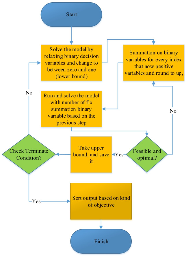
Fix-and-optimize solution approach (upper bound)

You know that constraint relaxation produces an upper bound, and the model’s output is equal to or greater than the main objective function ((Lotfi et al. 2021d). By fixing the binary variables, we obtain an appropriate upper bound that is bigger or equal to the main model (Helber & Sahling 2010).

The steps of fix-and-optimize are as follows:

1. Selecting and changing binary variable to linear (between zero and one) and obtaining optimal linear (relax constraint (27)),

2. We gain a lower bound after solving step 1, and our model is entirely linear,

3. Loop:

   1. Summarizing linear variables that we calculate in the previous step for each index and rounding them up,
   2. Solving the model with a new linear variable,
   3. If the model gains optimal value, we save the objective function as an upper bound in a list,
   4. Loop until stop criteria,

4. Sorting list based on ascending objective function and report list.

Using this algorithm makes to decreases the time solution. Therefore, this algorithm’s complexity includes removing binary variables, but free, non-negative variables and constraints are the same as Eqs. (37)–(39).

Results and discussion

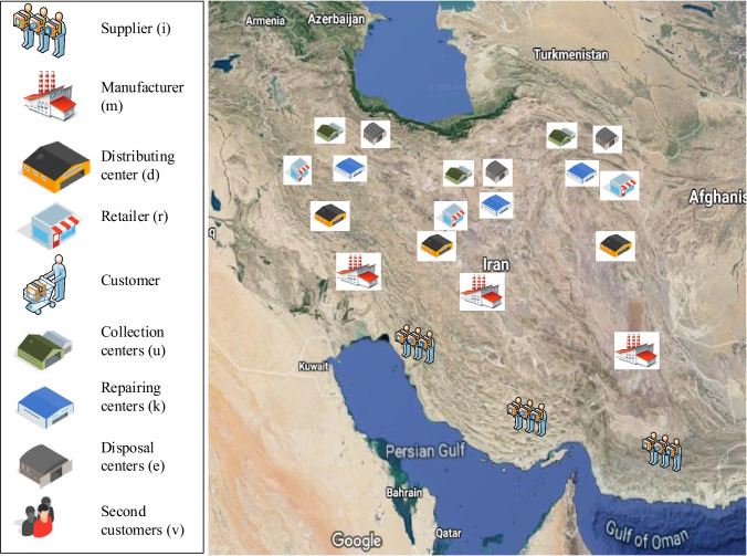
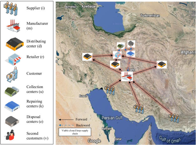
The case study of this research is the automotive industry. We mine data by running meetings with managers of the SC. Therefore, we assign parameter values in the notation list based on the case study information because there are many parameters. The automotive industry has value-added because of the process of materials. Consequently, we should keep these materials and return them to the economy. This subject is one of the circular economy pillars. In this case, we have a new company that wants to establish all components of CLSC, including customers, retailers, distributing centers, manufacturers, suppliers, recovery center, repairing center, disposal center, and second customer (Fig. 4). We applied the configuration: CPU 3.2 GHz, Processor Core i3-3210, 6.00 GB RAM, 64-bit operating system. We utilized the GAMS-CPLEX solver to attain optimal value. After running the model, we received cost and energy consumption and determined them in Table 2, Table 3, and Fig. 5. As can be seen, the cost function is 61369.620, and the energy consumption is 37.1553.

Fig. 4.

Suitable locations for the facilities

Table 2.

Number of sets, variables, and constraints of the case study

Problem	$\begin{array}{c}\left|i\right|.\left|m\right|.\left|d\right|.\left|r\right|.\left|u\right|.\\ \left|k\right|.\left|e\right|.\left|v\right|.\left|p\right|.\left|t\right|.\left|s\right|\\ \end{array}$	Binary var	Positive var	Free var	Constraint	Cost (TDollar)	Energy (MW)	Time (second)
P1-main	3.3.3.3.3.3.3.3.3.3.3	18	2031	31	1263	61,369.620	37.1553	1.758

Table 3.

Final location for the facility of VCLSC

Problem	Variables	City
P1	Supplier ($x{i}_i$)	Chabahar	Bandarabas	Abadan
		1	1	1
	Manufacture ($x{m}_m$)	Zahedan	Esfahan	Ilam
		0	1	0
	Distributing ($x{d}_d$)	Khoramabad	Esfahan	Birjand
		1	1	1
	Collection ($x{u}_u$)	Zanjan	Tehran	Mashhad
		0	1	0
	Repairing ($x{k}_k$)	Qazvin	Tehran	Sabzevar
		0	1	0
	Disposal ($x{e}_e$)	Rasht	Semnan	Ghochan
		0	1	0

Fig. 5.

Final location of the facility for VCLSC

Comparing viability and without viability

We compare the main problem in the situation with viability and without viability. As can be seen, the cost of P1-viable is less than P1-without considering viability and has a − 0.44% gap, and the energy consumption is greater than P1-without viable and has a 47.94% gap (cf. Table 4).

Table 4.

Compare model P1-viable and without viable

Model		P1-viable	P1-without viable	Gap
P1	Cost (TDollar)	61,369.6	61,637.3	-0.44%
	Energy (MW)	37.1553	19.3413	47.94%

Effects on the conservative coefficient

This section changes the conservative coefficient ($\beta$) between 0 and 100%. The cost function and energy consumption increase by increasing the conservative coefficient, and the time solution grows and then grows down (cf. Table 5, Fig. 6, Fig. 7, and Fig. 8).

Table 5.

Effects of conservative coefficient ($\beta$)

Problem	Conservative coefficient ($\beta$)	Cost (TDollar)	Energy (MW)	Time (second)	Cost variation
P1	0%	61,366.123	29.4147	0.408	− 0.01%
	25%	61,368.001	25.5527	0.933	− 0.003%
	50%	61,369.620	37.1553	1.758	0%
	75%	61,369.661	37.178	2.096	0.0001%
	100%	61,369.662	37.7643	1.078	0.0001%

Fig. 6.

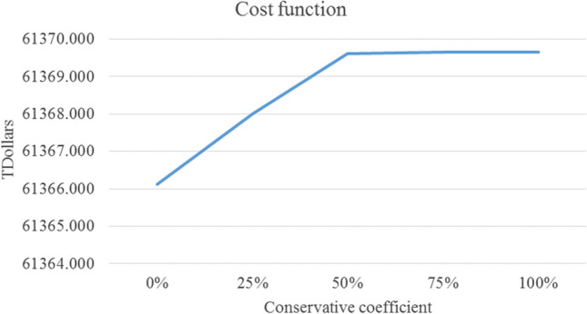
Effects of cost function based on conservative coefficient ($\beta$)

Fig. 7.

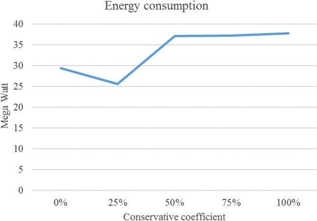
Effects of energy based on conservative coefficient ($\beta$)

Fig. 8.

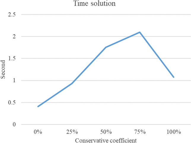
Effects of time solution based on conservative coefficient ($\beta$)

Effects on the confidence level

We change the confidence level ($\alpha$) between 1 and 10% in this section. The cost function and energy consumption increase by increasing the confidence level, and the time solution first increases and then grows down (cf. Table 6, Fig. 9, Fig. 10, and Fig. 11).

Table 6.

Effects of confidence level ($\alpha$)

Problem	Confidence level ($\alpha$)	Cost (TDollar)	Energy (MW)	Time (Second)	Cost variation
P1	1%	61,369.632	37.178	1.792	0.00%
	2%	61,369.627	37.178	0.693	0.000%
	5%	61,369.620	37.1553	1.758	0%
	8%	61,369.613	25.5527	1.043	0.0000%
	10%	61,369.496	25.5527	0.807	− 0.0002%

Fig. 9.

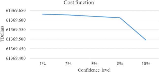
Effects of cost function based on confidence level ($\alpha$)

Fig. 10.

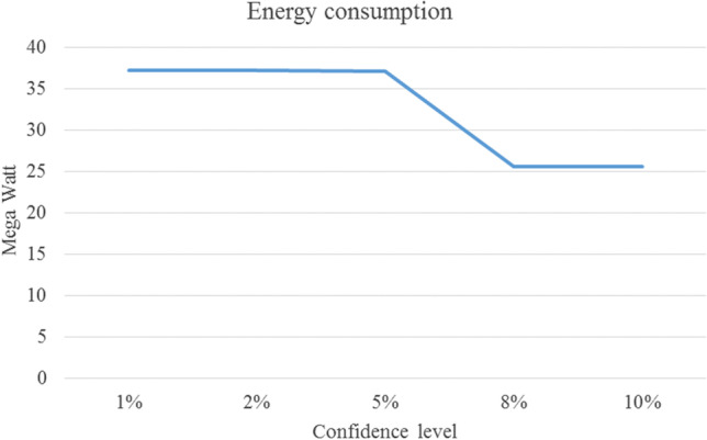
Effects of energy based on confidence level ($\alpha$)

Fig. 11.

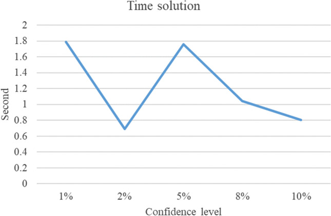
Effects of time solution based on confidence level ($\alpha$)

Effects on the maximum energy

This section changes the maximum energy (${\text{Emax}}_{\mathit{ts}}$) between 20 and 37 MW. Increasing the maximum allowed energy decreases the cost function (Table 7 and Fig. 12).

Table 7.

Effects of the allowed maximum energy

Problem	Maximum energy (MW)	Cost (TDollar)	Time (second)	Cost variation
P1	20.000	61,370.200	4.346	0.00095%
	21.667	61,369.635	6.479	0.00002%
	23.333	61,369.625	1.536	0.00001%
	33.333	61,369.620	1.27	0.00000%
	37.155	61,369.620	1.758	0%

Fig. 12.

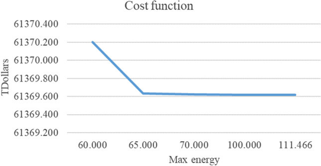
Effects of the cost function based on allowed maximum energy

Effects on the scale of the main model

In this section, we change the scale of the main model. By increasing the scale of the main model, the cost function, time solution, and energy consumption grow smoothly (cf. Table 8, Fig. 13, Fig. 14, and Fig. 15).

Table 8.

Cost and time solution for several problems

Problem	$\begin{array}{c}\left|I\right|.\left|M\right|.\left|D\right|.\left|R\right|.\left|U\right|.\\ \left|K\right|.\left|E\right|.\left|V\right|.\left|P\right|.\left|T\right|.\left|S\right|\\ \end{array}$	Binary variable	Positive variable	Free variable	Constraint	Cost (TDollar)	Energy (MW)	Time (second)
P1	3.3.3.3.3.3.3.3.3.3.3	18	2031	31	1263	61,369.6	37.1553	1.813
P2	4.4.4.4.4.4.4.4.4.4.3	24	6342	37	2937	63,735.2	68.194	11.866
P3	5.5.5.5.5.5.5.5.5.5.3	30	15,381	43	5691	68,872.3	146.085	30.37
P4	5.5.5.5.5.5.5.5.5.5.5	30	25,635	67	9479	63,577.8	194.781	141.752
P5	6.6.6.6.6.6.6.6.6.6.5	36	52,930	77	16,319	66,152.4	264.549	488.459
P6	7.7.7.7.7.7.7.7.7.7.3	42	58,659	55	15,519	63,755	225.192	331.039
P7	7.7.7.7.7.7.7.7.7.7.7	42	136,871	119	36,199	60,187.3	263.24	1999.56

Fig. 13.

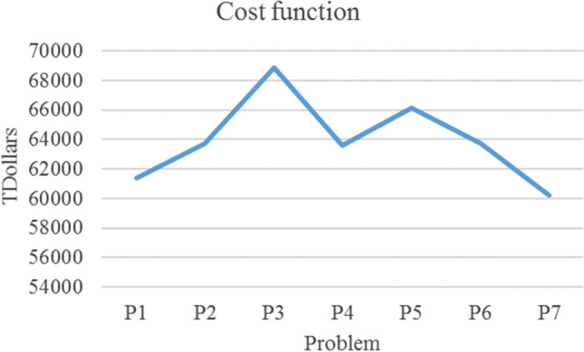
Effects of scale on cost function

Fig. 14.

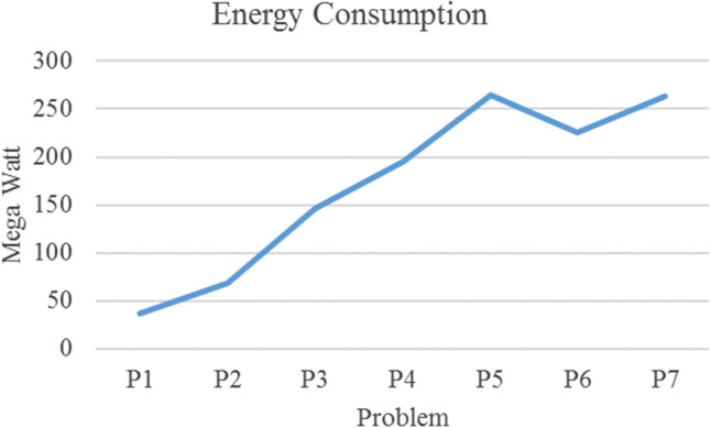
Effects of scale on energy consumption

Fig. 15.

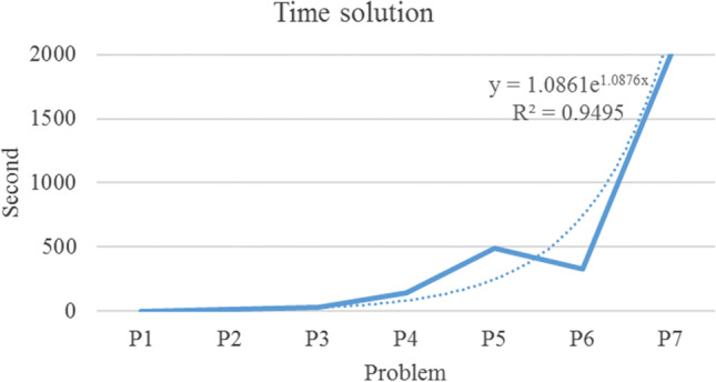
Effects of scale on-time solution

Upper bound for the main model

This section produces an appropriate upper bound for the large-scale problem. We suggested applying the Fix-and-Optimize algorithm (Lotfi et al., 2021b). As can be seen, the gap between this algorithm and the main problem for cost, energy, and time solution is approximately 6.10%, − 8.28%, and 75.01% (cf. Table 9, Fig. 16, Fig. 17, and Fig. 18).

Table 9.

Comparing the main model with the fix-and-opt algorithm

Problem	Main model (A)			Fix and opt. Upper bound (B)			Gap1%	Gap2%	Gap3%
	Cost (TDollar)	Energy (MW)	Time (second)	Cost (TDollar)	Energy (MW)	Time (second)
P1	61,369.6	37.1553	1.813	62,379.371	25.552	1.26	1.65%	− 31.23%	− 30.50%
P2	63,735.2	68.194	11.866	68,429.45	53.964	3.963	7.37%	− 20.87%	− 66.60%
P3	68,872.3	146.085	30.37	75,416.461	142.684	8.167	9.50%	− 2.33%	− 73.11%
P4	63,577.8	194.781	141.752	67,567.129	188.597	8.792	6.27%	− 3.17%	− 93.80%
P5	66,152.4	264.549	488.459	70,046.681	269.233	19.792	5.89%	1.77%	− 95.95%
P6	63,755	225.192	331.039	69,033.324	202.309	88.976	8.28%	− 10.16%	− 73.12%
P7	60,187.3	263.24	1999.56	62,457.67	284.295	160.723	3.77%	8.00%	− 91.96%
						Average	6.10%	− 8.28%	− 75.01%

Fig. 16.

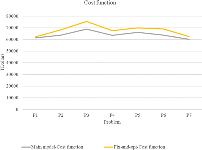
Comparing cost function of main model and fix-and-opt

Fig. 17.

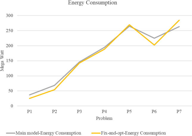
Comparing energy consumption of main model and fix-and-opt

Fig. 18.

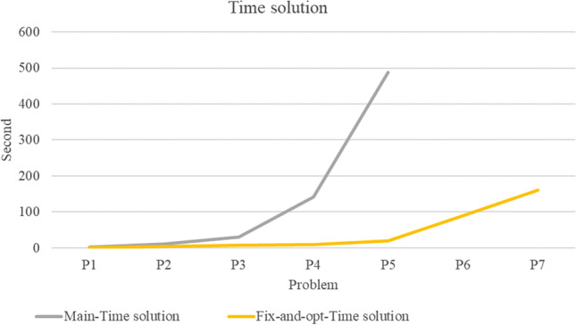
Comparing time solution of main model and fix-and-opt algorithm

Discussion

As can be seen, we show a CLSCND with a viable approach that integrates resiliency, sustainability, and agility for the first time. The case study is automotive production. The advantages of the model against the others given in the literature, we cannot see VCLSND in the literature review when surveying related work. There are only Lotfi et al. 2021d, f and Fazli-Khalaf et al. (2021) that are close to our research, but they did not consider agility and risk completely. We suggest both resilience strategies (the flexible capacity facility, multi-resource) that is not applied in the previous studies.

In addition, this model integrates resilience strategy through the flexible capacity facility, multi-resource (supplier and distribution), sustainable approach through presenting energy consumption constraints, and agile method by offering satisfaction demand. Also, we suggest a new form of cost function for robustness against demand disruption. This form includes minimizing the weighted expected, maximum, and EVaR cost function that was not considered in the previous study.

This research includes a VCLSCND that contains customers, retailers, distributing centers, manufacturers, suppliers, recovery centers, repairing centers, disposal centers, and second customers. We want to locate a resilience facility and determine flow quantity. Because we add agility constraints (satisfaction demand), resiliency constraints (multi-resource strategy and flexible capacity), and sustainability constraints (maximum allowed energy consumption), this model has a novel contribution and cannot compare with other models. As a result, we compare our model with a situation in which we do not consider viability. We found that the cost function of VCLSCND is almost − 0.44% less than without viability.

In addition, we run sensitivity analysis on essential parameters. Variation on the conservative coefficient shows that rising the conservative coefficient increases the cost function and energy. Variation in confidence level explains that the cost function and energy will decrease by increasing the confidence level. Increasing the maximum allowed energy reduces the cost function, too.

While variation on the scale of the model increases the cost function, time solution, and energy consumption grow smoothly. Finally, we produce an appropriate upper bound by the Fix-and-Opt algorithm for large-scale models. The gap between the upper bound and primary model is tiny.

Managerial insights and practical implications

In this section, we attract managers’ attention to managerial insights and practical implications. According to the environmental, energy, and social impacts on people’s lives, designing SCN is very important because SC affects production, employment, welfare, and posterity’s fate. One of the best models in this scope is the CLSC. The CLSC considers forward and backward products and returned products. This research shows VCLSC includes resiliency in facilities, environmental sustainability, and energy and agility in responsibility for the first time. Paying attention to resiliency makes it robust again demand and risk variation. The requirements of sustainability force to observe energy consumption, emission, and waste management. Although, we focus on the energy problem, one of Iran’s sustainable problems. Finally, we try to limit CLSC by energy constraints. Regarding resiliency, we utilized flexible capacity as a resiliency strategy. We added the rate of responsiveness as an agile constraint.

As a result, we compare our model with a situation in which we do not consider viability. We found that the cost function of VCLSCND is almost − 0.44% less than without viability. Also, Variation on the conservative coefficient shows that rising the conservative coefficient increases the cost function and energy. A variation in confidence level explains that the cost function and energy will decrease by increasing the confidence level. Increasing the maximum allowed energy reduces the cost function, too.

As SC managers, we should move to the viable SC and use methods to improve resiliency. Moreover, considering environmental requirements increase social responsibility. Finally, we need to design a global CLSC that observes all helpful concepts until resisting demand fluctuation and natural disasters.

Conclusions and outlook

This research suggests sustainability, agility, and resiliency for CLSC and develops VCLSC by considering risk and robustness in the circular economy for the first time. We applied a new robust stochastic optimization and a new form of robustness for the objective function. By minimizing the weighted expected, maximum, and EVaR cost function, we suggest robustness against demand fluctuation. Finally, we located suppliers, manufacturers, distributing, collection, repairing, and disposal centers. Eventually, we assigned flow on the forward and backward of CLSC.

The findings are as follows:

1. As can be seen, the cost of P1-viable is less than P1-without viable and has a − 0.44% gap and the energy consumption is greater than P1-without viable and has a 47.94% gap (cf. Table 4).

2. The cost function and energy consumption increase by increasing the conservative coefficient, and the time solution grows and then grows down (cf. Table 5, Fig. 6, Fig. 7, and Fig. 8).

3. The cost function and energy consumption increase by increasing the confidence level, and the time solution increases and then grows down (cf. Table 6, Fig. 9, and Fig. 10).

4. Increasing the allowed maximum energy decreases the cost function (cf. Table 7 and Fig. 12).

5. By increasing the scale of the main model, the cost function, time solution, and energy consumption grow smoothly (cf. Table 8, Fig. 13, Fig. 14, and Fig. 15).

6. We suggested applying Fix-and-Optimize algorithms. As can be seen, the gap between this algorithm and the main problem for cost, energy, and time solution is approximately 6.10%, − 8.28%, and 75.01% (cf. Table 9, Fig. 16, Fig. 17, and Fig. 18).

The limitation of this research is solving the large-scale in minimum time. It is better to use exact algorithms like Benders decomposition, Lagrange relaxation, and meta-heuristic algorithms (Fakhrzad & Lotfi 2018; Lotfi et al. 2017; Lotfi et al. 2021f). Eventually, we can suggest using other resilience and sustainable strategies, including green backup suppliers, decreasing node complexity, and trading carbon to increase resiliency and sustainability.

Furthermore, applying other risk criteria like robust conditional value at risk (RCVaR) helps consider the risk method (Lotfi et al. 2021b; Zare Mehrjerdi & Lotfi 2019). Other uncertainties like stochastic programming and robust optimization (convex) make it close to the real world (Lotfi et al. 2021c; Tirkolaee et al. 2021). In addition, fuzzy and a data-driven robust optimization approach is advantageous for a risk-averse decision-maker in the recent decade. Eventually, applying open innovation, learning, Internet-of-Thing (IoT) (De Vass et al. 2021), RFID, renewable energy (Lotfi et al. 2021b), and blockchain will improve SC agility, viability, and antifragility.

Author contribution

Reza Lotfi: conceptualization, supervision, software, methodology; software; formal analysis; data curation; writing original draft; visualization. Hossein Nazarpour: methodology; software; formal analysis; data curation; writing original draft; writing review and edit; visualization. Alireza Gharehbaghi: methodology, validation. Seyyed Mahdi Hosseini Sarkhosh: validation, writing review, and edit. Amirhossein Khanbaba: validation, writing review, and edit.

Data availability

The data and code supporting this study’s findings are openly available in VCLSC at http://doi.org/10.17632/t39mxddrg9.1 (Lotfi 2021).

Declarations

Ethics approval

Not applicable.

Consent to participate

Not applicable.

Consent for publication

Not applicable.

Competing interests

The authors declare no competing interests.

References

- De Vass T, Shee H, Miah SJ. Iot in supply chain management: a narrative on retail sector sustainability. Int J Log Res Appl. 2021;24(6):605–624. doi: 10.1080/13675567.2020.1787970. [DOI] [Google Scholar]
- Diabat A, Jebali A. Multi-product and multi-period closed loop supply chain network design under take-back legislation. Int J Prod Econ. 2021;231:107879. doi: 10.1016/j.ijpe.2020.107879. [DOI] [Google Scholar]
- Difrancesco RM, Huchzermeier A. Closed-loop supply chains: a guide to theory and practice. Int J Log Res Appl. 2016;19(5):443–464. doi: 10.1080/13675567.2015.1116503. [DOI] [Google Scholar]
- Fakhrzad M-B, Lotfi R. Green vendor managed inventory with backorder in two echelon supply chain with epsilon-constraint and NSGA-II approach. J Ind Eng Res Prod Syst. 2018;5(11):193–209. [Google Scholar]
- Fazli-Khalaf M, Naderi B, Mohammadi M, Pishvaee MS. The design of a resilient and sustainable maximal covering closed-loop supply chain network under hybrid uncertainties: a case study in tire industry. Environ Dev Sustain. 2021;23(7):9949–9973. doi: 10.1007/s10668-020-01041-0. [DOI] [Google Scholar]
- Fu R, Qiang QP, Ke K, Huang Z. Closed-loop supply chain network with interaction of forward and reverse logistics. Sustain Prod Consum. 2021;27:737–752. doi: 10.1016/j.spc.2021.01.037. [DOI] [Google Scholar]
- Helber S, Sahling F. A fix-and-optimize approach for the multi-level capacitated lot sizing problem. Int J Prod Econ. 2010;123(2):247–256. doi: 10.1016/j.ijpe.2009.08.022. [DOI] [Google Scholar]
- Hosseini S, Ivanov D, Dolgui A. Review of quantitative methods for supply chain resilience analysis. Transp Res Part E Logist Transp Rev. 2019;125:285–307. doi: 10.1016/j.tre.2019.03.001. [DOI] [Google Scholar]
- Ivanov, D. (2020). Viable supply chain model: integrating agility, resilience and sustainability perspectives—lessons from and thinking beyond the COVID-19 pandemic. Ann Oper Res 1–21 [DOI] [PMC free article] [PubMed]
- Ivanov D, Dolgui A. Viability of intertwined supply networks: extending the supply chain resilience angles towards survivability. A position paper motivated by COVID-19 outbreak. Int J Prod Res. 2020;58(10):2904–2915. doi: 10.1080/00207543.2020.1750727. [DOI] [Google Scholar]
- Kim YG, Do Chung B (2022) Closed-loop supply chain network design considering reshoring drivers. Omega 102610
- Lotfi R (2021) EcoVCLSC. Retrieved from: 10.17632/t39mxddrg9.1
- Lotfi R, Kargar B, Gharehbaghi A, Weber G-W (2021a) Viable medical waste chain network design by considering risk and robustness. Environ Sci Pollut Res 1–16 [DOI] [PMC free article] [PubMed]
- Lotfi R, Kargar B, Hoseini SH, Nazari S, Safavi S, Weber GW (2021b) Resilience and sustainable supply chain network design by considering renewable energy. Int J Energy Res
- Lotfi R, Mardani N, Weber GW (2021c) Robust bi‐level programming for renewable energy location. Inter J Energy Res
- Lotfi R, Mehrjerdi YZ, Mardani N. A multi-objective and multi-product advertising billboard location model with attraction factor mathematical modeling and solutions. Int J Appl Logistics (IJAL) 2017;7(1):64–86. doi: 10.4018/IJAL.2017010104. [DOI] [Google Scholar]
- Lotfi R, Mehrjerdi YZ, Pishvaee MS, Sadeghieh A, Weber G-W. A robust optimization model for sustainable and resilient closed-loop supply chain network design considering conditional value at risk. Numerical Algebra, Control & Optimization. 2021;11(2):221. doi: 10.3934/naco.2020023. [DOI] [Google Scholar]
- Lotfi, R., Safavi, S., Gharehbaghi, A., Ghaboulian Zare, S., Hazrati, R., & Weber, G.-W. (2021e). Viable supply chain network design by considering blockchain technology and cryptocurrency. Math Probl Eng 2021e
- Lotfi R, Sheikhi Z, Amra M, AliBakhshi M, Weber G-W (2021f) Robust optimization of risk-aware, resilient and sustainable closed-loop supply chain network design with Lagrange relaxation and fix-and-optimize. Int J Log Res Appl 1–41
- Mehrbakhsh S, Ghezavati V. Mathematical modeling for green supply chain considering product recovery capacity and uncertainty for demand. Environ Sci Pollut Res. 2020;27(35):44378–44395. doi: 10.1007/s11356-020-10331-z. [DOI] [PubMed] [Google Scholar]
- Mehrjerdi YZ, Shafiee M. A resilient and sustainable closed-loop supply chain using multiple sourcing and information sharing strategies. J Clean Prod. 2021;289:125141. doi: 10.1016/j.jclepro.2020.125141. [DOI] [Google Scholar]
- Nayeri S, Paydar MM, Asadi-Gangraj E, Emami S. Multi-objective fuzzy robust optimization approach to sustainable closed-loop supply chain network design. Comput Ind Eng. 2020;148:106716. doi: 10.1016/j.cie.2020.106716. [DOI] [Google Scholar]
- Nayeri S, Torabi SA, Tavakoli M, Sazvar Z (2021) A multi-objective fuzzy robust stochastic model for designing a sustainable-resilient-responsive supply chain network. J Clean Prod 127691
- Pahlevan SM, Hosseini SMS, Goli A (2021) Sustainable supply chain network design using products’ life cycle in the aluminum industry. Environ Sci Pollut Res 1–25 [DOI] [PubMed]
- Paul SK, Chowdhury P (2020) A production recovery plan in manufacturing supply chains for a high-demand item during COVID-19. Int J Phys Distrib Logist Manag
- Pourmehdi M, Paydar MM, Asadi-Gangraj E. Scenario-based design of a steel sustainable closed-loop supply chain network considering production technology. J Clean Prod. 2020;277:123298. doi: 10.1016/j.jclepro.2020.123298. [DOI] [Google Scholar]
- Rafigh P, Akbari AA, Bidhandi HM, Kashan AH (2021) Sustainable closed-loop supply chain network under uncertainty: a response to the COVID-19 pandemic. Environ Sci Pollut Res 1–17 [DOI] [PMC free article] [PubMed]
- Salehi-Amiri A, Zahedi A, Akbapour N, Hajiaghaei-Keshteli M. Designing a sustainable closed-loop supply chain network for walnut industry. Renew Sustain Energy Rev. 2021;141:110821. doi: 10.1016/j.rser.2021.110821. [DOI] [Google Scholar]
- Salehi-Amiri A, Zahedi A, Calvo EZR, Hajiaghaei-Keshteli M (2021b) Designing a Closed-loop Supply Chain Network Considering Social Factors; A Case Study on Avocado Industry. Appl Math Model
- Salehi-Amiri A, Zahedi A, Gholian-Jouybari F, Calvo EZR, Hajiaghaei-Keshteli M. Designing a closed-loop supply chain network considering social factors; a case study on avocado industry. Appl Math Model. 2022;101:600–631. doi: 10.1016/j.apm.2021.08.035. [DOI] [Google Scholar]
- Santander P, Sanchez FAC, Boudaoud H, Camargo M. Closed loop supply chain network for local and distributed plastic recycling for 3D printing: a MILP-based optimization approach. Resour Conserv Recycl. 2020;154:104531. doi: 10.1016/j.resconrec.2019.104531. [DOI] [Google Scholar]
- Simchi-Levi D, Simchi-Levi E (2020) We need a stress test for critical supply chains. Harvard Bus Rev 28
- Soleimani H, Mohammadi M, Fadaki M, Mirzapour Al-e-hashem SMJ (2021) Carbon-efficient closed-loop supply chain network: an integrated modeling approach under uncertainty. Environ Sci Pollut Res 1–16 [DOI] [PubMed]
- Srivastava M, Rogers H (2021) Managing global supply chain risks: effects of the industry sector. Int J Logist Res Appl 1–24
- Tehrani M, Gupta SM. Designing a sustainable green closed-loop supply chain under uncertainty and various capacity levels. Logistics. 2021;5(2):20. doi: 10.3390/logistics5020020. [DOI] [Google Scholar]
- Tirkolaee EB, Abbasian P, Weber G-W. Sustainable fuzzy multi-trip location-routing problem for medical waste management during the COVID-19 outbreak. Sci Total Environ. 2021;756:143607. doi: 10.1016/j.scitotenv.2020.143607. [DOI] [PMC free article] [PubMed] [Google Scholar]
- Tirkolaee EB, Goli A, Ghasemi P, Goodarzian F. Designing a sustainable closed-loop supply chain network of face masks during the COVID-19 pandemic: Pareto-based algorithms. J Clean Prod. 2022;333:130056. doi: 10.1016/j.jclepro.2021.130056. [DOI] [PMC free article] [PubMed] [Google Scholar]
- Tirkolaee EB, Goli A, Gütmen S, Weber G-W, Szwedzka K (2022b) A novel model for sustainable waste collection arc routing problem: Pareto-based algorithms. Ann Oper Res 1–26 [DOI] [PMC free article] [PubMed]
- Yavari M, Ajalli P. Suppliers’ coalition strategy for green-resilient supply chain network design. J Ind Prod Eng. 2021;38(3):197–212. [Google Scholar]
- ZareMehrjerdi Y, Lotfi R. Development of a mathematical model for sustainable closed-loop supply chain with efficiency and resilience systematic framework. Int J Supply Oper Manag. 2019;6(4):360–388. [Google Scholar]
Associated Data
This section collects any data citations, data availability statements, or supplementary materials included in this article.
Data Availability Statement