GAPIT Version 3: Boosting Power and Accuracy for Genomic Association and Prediction

Abstract

Genome-wide association study (GWAS) and genomic prediction/selection (GP/GS) are the two essential enterprises in genomic research. Due to the great magnitude and complexity of genomic and phenotypic data, analytical methods and their associated software packages are frequently advanced. GAPIT is a widely-used genomic association and prediction integrated tool as an R package. The first version was released to the public in 2012 with the implementation of the general linear model (GLM), mixed linear model (MLM), compressed MLM (CMLM), and genomic best linear unbiased prediction (gBLUP). The second version was released in 2016 with several new implementations, including enriched CMLM (ECMLM) and settlement of MLMs under progressively exclusive relationship (SUPER). All the GWAS methods are based on the single-locus test. For the first time, in the current release of GAPIT, version 3 implemented three multi-locus test methods, including multiple loci mixed model (MLMM), fixed and random model circulating probability unification (FarmCPU), and Bayesian-information and linkage-disequilibrium iteratively nested keyway (BLINK). Additionally, two GP/GS methods were implemented based on CMLM (named compressed BLUP; cBLUP) and SUPER (named SUPER BLUP; sBLUP). These new implementations not only boost statistical power for GWAS and prediction accuracy for GP/GS, but also improve computing speed and increase the capacity to analyze big genomic data. Here, we document the current upgrade of GAPIT by describing the selection of the recently developed methods, their implementations, and potential impact. All documents, including source code, user manual, demo data, and tutorials, are freely available at the GAPIT website (http://zzlab.net/GAPIT).

Introduction

Computer software is essential for genomic research. Genome-wide association study (GWAS) and genomic prediction (GP) are the two essential enterprises for genomic research. For a particular trait of interest, GWAS focuses on finding genetic loci associated with the markers (typically single nucleotide polymorphisms; SNPs) and estimating their effects. GP, known as genomic selection (GS) in the fields of animal and plant breeding, focuses on the direct prediction of phenotypes by estimating the total genetic merit underlying the phenotypes [1]. The estimated genetic merit is also known as the estimated breeding value (EBV) for animal and plant breeding. In the long term, the assessment of all genetic loci underlying a trait may eventually lead to highly accurate EBV predictions. In the short term, methods have been developed to derive EBV even without identifying the associated genetic loci. Consequently, some statistical methods are shared between GWAS and GS, and some methods are specific to each. Accordingly, the software packages are also characterized into GWAS-specific, GS-specific, or packages that perform both.

For GWAS, many statistical methods and software packages have been developed to improve computational efficiency, statistical power, and control of false positives [2]. The most computationally efficient method is the general linear model (GLM), which can fit population structure or principal components as fixed effects to reduce the false positives caused by population stratification [3], [4]. To account for the relationships among individuals within sub-populations, kinship among individuals was introduced through the mixed linear model (MLM) by using genetic markers covering the entire genome [5]. This strategy serves to further control false positives. To reduce the computational burden of MLM, many algorithms have been developed, including efficient mixed model association (EMMA) [6], EMMA eXpredited (EMMAx), population parameter previously determined (P3D) [7], [8], factored spectrally transformed linear mixed models (FaST-LMM) [9], and genome-wide rapid association using mixed model and regression (GRAMMAR) [10]. These methods improve computing efficiency of MLM, but their statistical power remains the same as MLM.

Enhancement of MLM has also been introduced to improve statistical power. To reduce the confounding bias between kinship and testing markers, individuals in the MLM are replaced with their corresponding groups in the compressed MLM (CMLM), which also improves computing efficiency [8]. Referring to the clustering method to fit such relationship between individuals, the enriched CMLM (ECMLM) was developed to further improve statistical power [11]. Instead of using all markers to derive kinship among individuals across traits of interest, selection of the markers according to traits of interest can improve statistical power. One of such methods is settlement of MLMs under progressively exclusive relationship (SUPER) [12]. SUPER contains three steps. The first step is the same as in other models such as GLM or MLM, i.e., to have an initial assessment of the marker effects. In the second step, kinship is optimized using maximum likelihood in a mixed model with kinship derived from the selected markers based on their effects and relationship on linkage disequilibrium (LD). In the third step, markers are tested again one at a time as final output, with kinship derived from the selected markers except the ones that are in LD with the testing markers.

Same as the extension of single-marker tests using GLM to stepwise regression, e.g., GLMSELECT procedure in the Statistical Analysis System (SAS) [13], [14], single-locus tests using MLM were also extended to multi-locus tests, named multiple loci mixed model (MLMM) [15]. The most significant maker is fitted as a covariate in the stepwise fashion. Iteration stops when variance associated with the kinship goes to zero, followed by a backward stepwise regression to eliminate the non-significant covariate markers. In MLMM, both covariate markers and kinship are fitted in the same MLM. An iterative method named as fixed and random model circulating probability unification (FarmCPU) [16] also uses stepwise strategy to estimate marker effect. Different from MLMM, FarmCPU iterates back and forth with two models. One model is an MLM, which contains the random effect associated with kinship and covariates such as population structure, but not the associate markers. The associated markers are optimized to derive the kinship using maximum likelihood. The other model is a GLM, which contains a testing marker and covariates such as population structure. Since a marker test in GLM does not involve kinship, FarmCPU is not only faster but also provides higher statistical power than MLMM. The MLM in FarmCPU is further replaced with GLM to speed up the computation in the new method named Bayesian-information and LD iteratively nested keyway (BLINK) [17]. The maximum likelihood method in MLM is replaced by the Bayesian-information content. BLINK eliminates the restriction assuming that causal genes are evenly distributed across the genome by SUPER and FarmCPU method, consequently boosting statistical power.

For GP/GS, the earliest effort can be traced to the use of marker-based kinship in the best linear unbiased prediction (BLUP) method, currently known as genomic BLUP or gBLUP [18], [19], [20]. The method uses all markers covering the whole genome to define the kinship among individuals to estimate their EBVs. A different strategy is to estimate the effects of all markers and sum them together to predict the total genetic effects of all individuals [21]. To avoid the overfitting problem in the fixed-effect model, these markers are fitted as random effects simultaneously. A variety of restrictions and assumptions are applied to these random effects and their prior distributions under the Bayesian theorem. Different methods are named according to different prior probability, such as Bayes A, B, Cpi, and least absolute selection and shrinkage operator (LASSO) [21]. The case assuming that effects of all markers have the same distribution with constant prior variance is equivalent to ridge regression [19], [22].

Development of many software packages is accompanied by the development of GWAS and GS methods. Therefore, these methods and software packages are often given the same name, such as EMMA [6], EMMAx [7], FaST-LMM [9], FarmCPU [16], and BLINK [17]. Often, to compare different statistical methods, users must learn how to use various software packages. To reduce the multiple steep learning curves for users, some packages are developed with more than one statistical method. These packages include population-based linkage tool (PLINK) with GLM and logistic regression [23]; trait analysis by association, evolution and linkage (TASSEL) [24] with GLM and MLM; ridge regression BLUP (rrBLUP) with ridge regression and gBLUP [22]; as well as Bayesian generalized linear regression (BGLR) with ridge regression, gBLUP, and Bayesian methods [25]. Also, some packages have implemented methods for both GWAS and GS so that users can use one software package to conduct both analyses. One example is genome association and prediction integrated tool (GAPIT). GAPIT was initiated with GLM, MLM, EMMAx/P3D, CMLM, and gBLUP in version 1 (GAPIT1) [26] and enriched with ECMLM, FaST-LMM, and SUPER in version 2 (GAPIT2) [27].

Furthermore, with such a variety of methods available, researchers feel extremely overwhelmed when trying to choose the best method to analyze their particular data. This dilemma is especially true when only a subset of these methods has been compared under conditions less relevant to a researcher’s specific study conditions. For example, simulation studies have demonstrated that FarmCPU is superior to MLMM for GWAS [16]; however, no comparisons have been conducted between SUPER and FarmCPU or between SUPER and MLMM. Similarly, for GS, gBLUP, SUPER BLUP (sBLUP), and compressed BLUP (cBLUP) have been compared with Bayesian LASSO [1]. Thus, software packages with features that allow researchers to conduct comparisons for model selection — especially under the conditions relevant to their studies — are critically needed.

To address these critical needs, we continuously strive to upgrade GAPIT software by adding state-of-the-art GWAS and GS methods as they become available. Herein, we report our most recent efforts to upgrade GAPIT to version 3 (GAPIT3) by implementing MLMM, FarmCPU, and BLINK [15], [16], [17] for GWAS, as well as sBLUP and cBLUP for GS [1]. We also added features that allow users to interact with both the analytical methods and display outputs for comparison and interpretation. Users’ prior knowledge can now be used to enhance method selection and unfold the discoveries hidden by static outputs.

Method

Architecture of GAPIT3

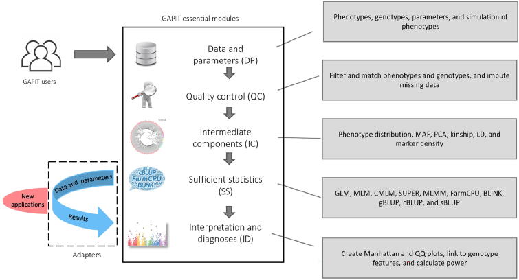
To implement three multi-locus GWAS methods (MLMM, FarmCPU, and BLINK) and two new methods of GS (cBLUP and sBLUP), we redesigned GAPIT with a new architecture to easily incorporates an external software package. In the order of execution, GAPIT is compartmentalized into five modules: 1) data and parameters (DP); 2) quality control (QC); 3) intermediate components (IC); 4) sufficient statistics (SS); and 5) interpretation and diagnoses (ID). Any of these modules are optional and can be skipped. However, GAPIT3 does not allow modules to be executed in reverse order (Fig. 1).

Fig. 1.

GAPIT essential modules and adapters to external packages. GAPIT version 3 was designed to have five sequential modules and multiple adapters that connect external software packages. The first module (DP) is responsible to process input data and parameters from users. The second module (QC) is responsible for quality control, including missing genotype imputation. The third module (IC) provides intermediate results, including MAF, PCA, kinship, LD analysis, and maker density distribution. The fourth module (SS) contains multiple adapters that convert input data into sufficient statistics, including maker effects, P values, and predicted phenotypes. The current adapters include GLM, MLM, CMLM, SUPER, MLMM, FarmCPU, BLINK, gBLUP, cBLUP, and sBLUP. The fifth module (ID) provides the interpretation and diagnosis on the final results, including P values illustrated as Manhattan plots and QQ plots. GAPIT, genomic association and prediction integrated tool; DP, data and parameters; QC, quality control; IC, intermediate components; MAF, minor allele frequency; PCA, principal component analysis; LD, linkage disequilibrium; GLM, general linear model; MLM, mixed linear model; CMLM, compressed MLM; SUPER, settlement of MLM under progressively exclusive relationship; MLMM, multiple loci mixed model; FarmCPU, fixed and random model circulating probability unification; BLINK, Bayesian-information and LD iteratively nested keyway; gBLUP, genomic best linear unbiased prediction; cBLUP, compressed BLUP; sBLUP, SUPER BLUP; QQ, quantile–quantile.

The DP module contains functions to interpret input data, input parameters, genotype format transformation, missing genotype imputation, and phenotype simulations. The types of input data and their labels are the same as previous versions of GAPIT, including phenotype data (Y); genotype data in either haplotype map (HapMap) format (G), or numeric data format (GD) with genetic map (GM); covariate variables (CV), and kinship (K). The input parameters include those from previous GAPIT versions plus the parameters for the new GWAS and GS methods and the enrichments associated with the other four modules. Two genetic models, additive and dominant, are available to transform genotypes in HapMap format into numeric format. Under the additive model, homozygous genotypes with recessive allele combinations are coded as 0, homozygous genotypes with dominant allele combinations are coded as 2, and heterozygous genotypes are coded as 1. Under the dominant model, both types of homozygous genotypes are coded as 0 and heterozygous genotypes are coded as 1. When genotype, heritability, and number of quantitative trait nucleotides (QTNs) are provided without phenotype data, GAPIT3 conducts a phenotype simulation from the genotype data.

By default, GAPIT assumes that users would provide quality data and thus does not perform data quality control. When the QC option is turned on, GAPIT conducts QC on imputing missing genotypes, filtering markers by minor allele frequency (MAF), sorting individuals in phenotype and genotype data, as well as matching the phenotype and genotype data together. GAPIT provides multiple options for genotype imputation, including major homozygous genotypes and heterozygous genotypes.

In the IC module, GAPIT provides comprehensive functions to generate intermediate graphs and reports, including phenotype distribution, MAF distribution, heterozygosity distribution, marker density, LD decay, principal components, and kinship. These reports and graphs help users to diagnose and identify problems within the input data for QC. For example, an associated marker should be further investigated if it has low MAF.

The SS module contains multiple adapters that generate SS for existing methods in the previous versions of GAPIT and new external methods. The statistics include the estimated effect, P values of all markers for GWAS, and predicted phenotypes of individuals for GS. The methods in the previous versions include GLM, MLM, CMLM, ECMLM, SUPER, and gBLUP. The new adapters developed in GAPIT3 include MLMM, FarmCPU, BLINK, cBLUP, and sBLUP.

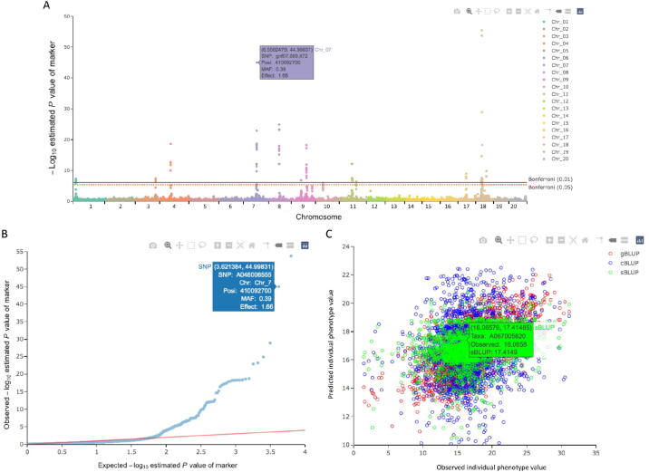
The ID module contains the static reports developed in previous GAPIT versions and the new interactive reports generated in GAPIT3. The interactive reports include the rotational 3D plot of the first three principal components, display of marker information on Manhattan plots and quantile–quantile (QQ) plots, and individual information on the phenotype plots (predicted vs. observed). The marker information includes maker name, chromosome, position, MAF, P value, and estimated effect. The individual information covers the individual name and the values for predicted and observed phenotypes.

Implementation of MLMM and FarmCPU

Both MLMM and FarmCPU have source code available on their respective websites. These source codes are directly integrated into the GAPIT source code, so users are only required to install GAPIT3, not three packages separately (GAPIT3, MLMM, and FarmCPU). Integrating MLMM and FarmCPU source code into GAPIT source code lowers the risk of breaking the linkage between GAPIT and these two software packages when they release updates. The disadvantage in doing so is that MLMM and FarmCPU source codes remain static in GAPIT. To compensate for this disadvantage, the GAPIT team periodically checks for updates of these two packages and updates the GAPIT source code accordingly.

Implementation of BLINK R and C versions

BLINK R version is released as an executable R package on GitHub. GAPIT accesses BLINK R as an independent package. Similarly, BLINK C version is released as an executable C package on GitHub. To access BLINK C, GAPIT needs the executable program in the working directory. To avoid the potential risk of breaking the linkage between GAPIT and BLINK, the GAPIT team maintains a close connection with the BLINK team for updates. BLINK C conducts analyses on binary files for genotypes. The binary files not only make BLINK C faster, but also provide the capacity to process big data with limited memory. Running BLINK C through GAPIT requires nonbinary files first, then BLINK C is used to convert them to binary. For big data, we recommend directly accessing BLINK C to obtain P values and using the GAPIT ID module to interpret and diagnose the results.

Implementation of cBLUP and sBLUP

cBLUP and sBLUP were developed from the corresponding GWAS methods: CMLM and SUPER, respectively. Since CMLM and SUPER have already been implemented in GAPIT GAPIT1 and GAPIT2, respectively, implementation of cBLUP and sBLUP is more straightforward than other implementations. For cBLUP, the solutions of the random group effects in CMLM are used as the genomic EBVs for the corresponding individuals. For sBLUP, the calculation is even easier than the SUPER GWAS method. For the SUPER GWAS method, a complementary kinship is used for a testing SNP that is in LD with some of the associated SNPs. For sBLUP, all associated markers are used to derive the kinship and subsequently to predict the EBVs and phenotype values of individuals. No operation for the complementary process is necessary.

Implementation of interactive reports

Two types of interactive reports are included in GAPIT3. First, users can now interact with Manhattan plots, QQ plots, and scatter plots of predicted vs. observed phenotypes to extract information about markers and individuals. For example, by moving the cursor or pointing device over a data point, users can find names and positions of markers, or names and phenotypes of individuals. An R package plotly is used to store this type of information in the format of HTML files, which can be displayed by web browsers. Second, users can rotate graphs such as 3D principle component analysis (PCA) plots using a pointing device such as mouse or trackpad. The R packages (rgl and rglwidget) are jointly used to plot 3D figures.

Percentage of variance explained

In GAPIT3, the percentage of total phenotypic variance explained (PVE) by significantly associated markers (P values < Bonferroni threshold) is evaluated. A Bonferroni multiple test threshold is used to determine significance. The associated markers are fitted as random effects in a multiple random variable model. The model also include other fixed effects that are used in GWAS to select the associated markers. The multiple random variable model is analyzed using an R package, lme4, to estimate the variance of residuals and the variance of the associated markers. The percentage explained by the markers are calculated as their corresponding variance divided by the total variance, which is the sum of residual variance and the variance of the associated markers.

Results

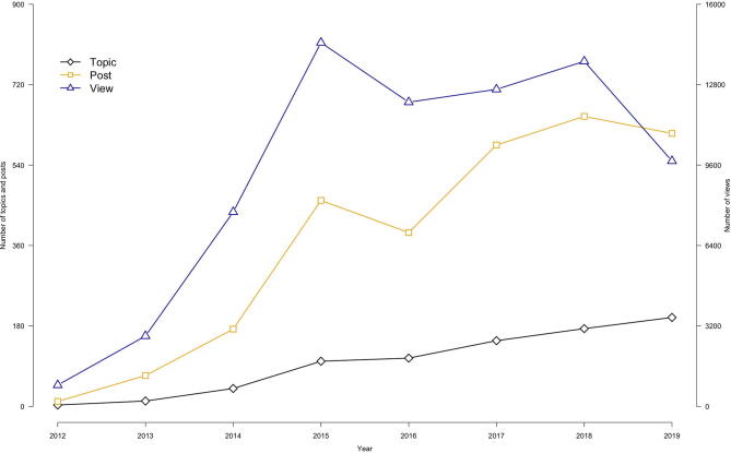
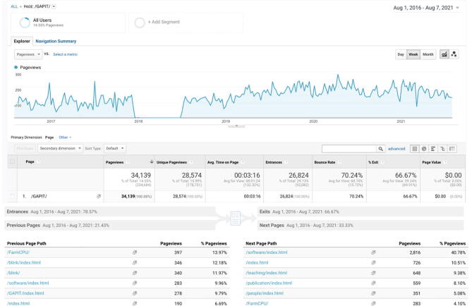
GAPIT is a widely used software package. GAPIT website (https://zzlab.net/GAPIT) has received over 34,000 pageviews since 2016. The GAPIT forum (https://groups.google.com/g/gapit-forum) on Google contains ∼ 2900 posts that cover ∼ 800 topics (regarding the usage, functions, bugs, and fixes) and had been viewed ∼ 74,000 times by the GAPIT community between 2012 and 2019 (Figures S1 and S2). Meanwhile, articles on GAPIT1 and GAPIT2 received 1250 and 203 citations, respectively. The GAPIT3 project started after the publication of GAPIT2 in 2016. Since then, we have implemented three multi-locus methods for GWAS and two methods for GS (Fig. 2). In addition, we have enhanced the outputs of GAPIT to improve their quality, and to help users to more easily diagnose the data quality, compare analytical methods, and interpret the results.

Fig. 2.

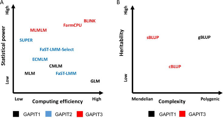
Statistical methods implemented in previous and current versions of GAPIT. The statistical methods are characterized by statistical power and computing efficiency (A) for GWAS and by genetic architecture of targeting traits for GS with respect to heritability and complexity (B). The GWAS methods include GLM, MLM, CMLM, FaST-LMM, FaST-LMM-Select, ECMLM, SUPER, MLMM, FarmCPU, and BLINK. The GS methods include the regular gBLUP, cBLUP, and sBLUP. Methods implemented in the initial version of GAPIT, newly in GAPIT2, and newly in the current GAPIT3 are indicated with letters in black, blue and red, respectively. GWAS, genome-wide association study; GS, genomic selection; FaST-LMM, factored spectrally transformed linear mixed models; FaST-LMM-Select, FaST-LMM select; ECMLM, enriched CMLM.

Implementation of GWAS and GS methods

GAPIT1 was initiated with the single-locus test based on the GLM, MLM, and CMLM. The computation complexity of MLM is cubic to the number of individuals. Thus, compression of individuals to groups not only improves statistical power, but also dramatically reduces computing time (Fig. 2A). To improve the computing speed of MLM, GAPIT2 implemented FaST-LMM, which uses a set of markers to define kinship without performing the actual calculations.

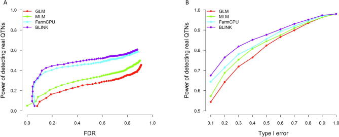
All GWAS methods implemented in GAPIT1 and GAPIT2 are based on the single-locus testing. In GAPIT3, we implemented all three of multi-locus test methods (MLMM, FarmCPU, and BLINK). We simulated 100 traits and ran four methods (GLM and MLM are single-locus methods, FarmCPU and BLINK are multi-locus methods). Power against false discover rate (FDR) and power against type I error are used to compare the performance differences between single-locus and multi-locus methods (Figure S3).

For GP/GS, GAPIT1 and GAPIT2 implement gBLUP using MLM. This method works well for traits controlled by many genes, but not as well for traits controlled by a small number of genes. To overcome this difficulty, the updated GAPIT3 implements the sBLUP method, which is superior to gBLUP for traits controlled by a small number of genes [1]. Both gBLUP and sBLUP have a disadvantage for traits with low heritability. Therefore, GAPIT3 implements the cBLUP method [1], which is superior to both gBLUP and sBLUP for traits with low heritability (Fig. 2B).

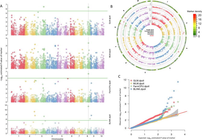
The new GAPIT3 creates two types of Manhattan plots, the standard orthogonal type with x- and y-axes (Figure S4A), and a circular type (Figure S4B) that takes less display space. The overlap in results between multiple methods is displayed as either solid or dashed vertical lines that will extend through the Manhattan plots for all methods (Figure S4). A solid vertical line indicates that the overlap of significant SNP is shared by more than two methods and a dashed vertical line indicates the overlap only occurs between two methods. When multiple traits are analyzed with a single method, the trait results are displayed in the same style as multiple methods. When both multiple methods and multiple traits are employed, the method plots are nested within the trait plots. We summarized the methods parameters and steps in the new GAPIT3 (Table 1).

Table 1.

Characteristics of methods in GAPIT3.

Method	Testing marker	No. of steps	Model	Kinship
GLM	Single locus	One	Fixed	NA
MLM	Single locus	One	Mixed	All markers
CMLM	Single locus	One	Mixed	Individuals clustered into groups
ECMLM	Single locus	One	Mixed	Individuals clustered into groups by enrichment
SUPER	Single locus	Two	Mixed	All marker except pseudo QTNs
MLMM	Multiple loci	Iterative	Mixed	All markers
FarmCPU	Multiple loci	Iterative	Fixed and mixed	Pseudo QTNs
BLINK	Multiple loci	Iterative	Fixed	NA
gBLUP	NA	One	Mixed	All markers for all individuals
cBLUP	NA	One	Mixed	Individuals clustered into groups with all markers
sBLUP	NA	One	Mixed	Pseudo QTNs

Note: NA, not applicable; GLM, general linear model; MLM, mixed linear model; CMLM, compressed MLM; ECMLM, enrichment CMLM; SUPER, settlement of MLMs under progressively exclusive relationship; MLMM, multiple loci MLM; FarmCPU, fixed and random model circulating probability unification; BLINK, Bayesian-information and linkage-disequilibrium iteratively nested keyway; gBLUP, genomic best linear unbiased prediction; cBLUP, compressed BLUP; sBLUP, SUPER BLUP; QTN, quantitative trait nucleotide.

Adaptation of existing GAPIT users

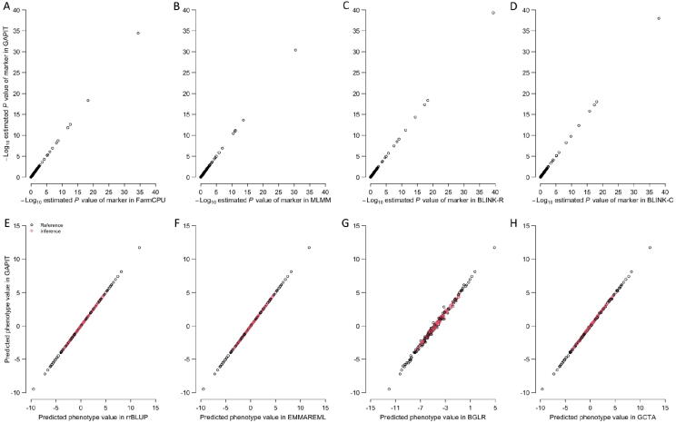
Users already familiar with GAPIT software have experienced no difficulty in migrating to GAPIT3. Experiences of using other related software packages also help to use GAPIT. GAPIT generated identical results for the same methods implemented in the separated packages (Fig. 3). By default, GAPIT3 conducts GWAS using the BLINK method, which has the highest statistical power and computing efficiency among all methods implemented. Users can change the default to other methods by including a model statement. For example, to use the FarmCPU method, users would include the statement “model = “FarmCPU”” to override the default. The model options include GLM, MLM, CMLM, ECMLM, FaST-LMM, FaST-LMM-Select, SUPER, MLMM, FarmCPU, and BLINK.

Fig. 3.

Comparison of P values and predicted phenotype values using GAPIT and other software packages. The comparison was conducted on a trait simulated from the genotypes of 3093 SNPs on 281 maize lines (GAPIT demonstration datasets, https://zzlab.net/GAPIT/GAPIT_Tutorial_Data.zip). The simulated trait had 75% heritability with 20 QTNs. P values obtained are log transformed and compared between GAPIT (vertical axis) and four software packages (horizontal axis) for GWAS analysis that were run as standalone packages, including FarmCPU, MLMM, BLINK R version, and BLINK C version. Similarly, predicted phenotype values using GAPIT are compared with those predicted using four software packages that were run as standalone packages, including rrBLUP, EMMAREML, BGLR, and GCTA. QTN, quantitative trait nucleotide; rrBLUP, ridge regression BLUP; EMMAREML, efficient mixed model with restricted maximum likelihood; BGLR, Bayesian generalized linear regression; GCTA, genome-wide complex trait analysis.

GAPIT can also conduct GWAS and GS with multiple methods in a single analysis, allowing comparisons among methods for selection. For example, when the five methods (GLM, MLM, CMLM, FarmCPU, and BLINK) are used on maize flowering time in the demo data, inflation of P values and power of the analyses can be compared with Manhattan plots side-by-side (Figure S4). All plots for the multiple methods showed an interconnected vertical line that runs through chromosome 8. The results showed that the GLM method identified association signals above the Bonferroni threshold (horizontal solid green line in each plot). However, the association signals were inflated across the genome (the red dots on the QQ plots in the Figure S4C). BLINK method also identified two associated markers, including the marker close to a flowering time gene, VGT1 on chromosome 8. The QQ plot suggests that 99% of the markers have P values below the expected P values, which are indicated by the solid red line.

Assessment of explained variance

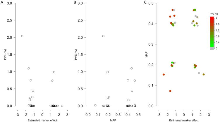
GAPIT1 outputs the proportion of the regression sum of squares of testing markers to the total sum of squares as the estimate of variance explained by the markers. This approach is debatable because the sum of these proportions can exceed 100% when multiple markers are tested independently. In GAPIT2, this output is suppressed. However, we received substantial demands from GAPIT users for such output because some journals and reviewers require this information. To solve both of these problems, GAPIT3 conducts additional analyses using all associated markers as random effects. The proportion of variance of a marker over the total variance, including the residual variance, is reported as the proportion of total variance explained by the markers. This guarantees the sum of proportions of variance explained by the associated markers is below 100%. The non-associated markers are considered to contribute nothing to the total variance. The percentage of PVE by a marker is correlated with its MAF and magnitude of marker effect. These relationships are demonstrated by scatter plots and a heatmap (Fig. 4). The heat map indicates which markers explain a high proportion of the variance due to either a high MAF or a large magnitude of effect, or both.

Fig. 4.

PVE by associated markers. GAPIT 3 provides estimates of the percentage of PVE by associated markers. The proportion is a function of both magnitude of marker effects and MAF. Larger marker effects and larger MAF contribute to larger proportion of phenotypic variance explained. This relationship is demonstrated on a trait simulated from the mouse genotypes of 12,564 SNPs on 1440 individuals (available at http://gscan.well.ox.ac.uk). The simulated trait had 75% heritability with 20 QTNs. A. Markers with large magnitude that explain little phenotypic variances due to low MAF. B. Markers with large MAF that explain little phenotypic variances due to small effect. C. Markers away from the center where both MAF and marker effect are zeros that explain more variation. PVE, phenotypic variance explained.

Enriched report output

When viewing the output graphics, such as Manhattan plots, QQ plots, and scatter plots of predicted vs. observed phenotypes, users are interested in the names and properties of markers and individuals. Finding this information usually requires computer programming to extract data from multiple resources, which includes searching files for P values, genotypes, estimated effects, and MAFs. With GAPIT3, in the interactive result, all information can be found by moving the cursor over the data point of interest (Fig. 5, Figure S5). For example, on the Manhattan and QQ plots, when the cursor moves over a data point, the marker information is displayed. The Manhattan plot also contains a chromosome legend. Chromosomes can be hidden or displayed with different mouse clicking patterns.

Fig. 5.

Interactive extraction of information for markers and individuals. GAPIT3 outputs two interactive HTML files to help user to extract information of markers on Manhattan plots (A) and QQ plots (B). The interactive plots are demonstrated on a trait simulated from the mouse genotypes with 12,564 SNPs on 1440 individuals (available at http://gscan.well.ox.ac.uk). The simulated trait had 75% heritability with 20 QTNs. When the cursor is moved over a dot, the marker information is displayed instantly, including name, P values, chromosome, position, and MAF. Similarly, a HTML file is generated to display the predicted phenotypes against observed phenotypes (C). When the cursor is moved over a dot, the individual information is displayed instantly, including name, as well as predicted and observed phenotypic values. When multiple prediction methods are used, individuals are displayed as different colors for different methods, such as gBLUP, cBLUP, and sBLUP.

Computing time

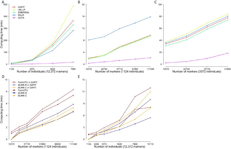
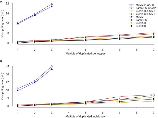
GAPIT3 newly implements three multi-locus test methods (MLMM, FarmCPU, and BLINK) for GWAS and two methods (cBLUP and sBLUP) for GS. All methods (GWAS and GS) have linear computing time to number of markers (Fig. 6, Figure S6). However, they have mixed computing complexity to number of individuals. Most of these methods have computing time complexity that are cubic to number of individuals, including gBLUP and cBLUP for GS, and MLMM for GWAS. For execution of gBLUP, genome-wide complex trait analysis (GCTA) was vigorous under all conditions to other packages, including BGLR, efficient mixed model with restricted maximum likelihood (EMMREML), GAPIT, and rrBLUP. All of these packages have linear computing time to number of markers, and nonlinear time to number of individuals. Their order changes depending on the number of individuals due to different setting cost. With number of markers duplicated four times and number of individuals duplicated at multiple levels (12×, 20×, and 28 × ), the computing time shows nonlinear relationship with the number of individuals, except the GCTA package (Fig. 6A). For small number of individuals (1124), BGLR was the slowest. When number of individuals is increased to three-fold (1124 × 3), rrBLUP becomes the slowest (Fig. 6B and C). Therefore, GCTA is recommended for gBLUP, and GAPIT is preferred over other methods for using cBLUP and sBLUP. There are only two methods that have linear computing time to number of individuals: FarmCPU and BLINK (Fig. 6D and E). There is a modest increase in computing time when using MLMM, FarmCPU, and BLINK packages within GAPIT, compared to using these packages directly. There are two versions for BLINK methods: C version and R version. Previous studies have demonstrated that the C version is much faster than the R version when they are operated as standard alone [17]. When they are executed within GAPIT, this situation is reversed. This is because GAPIT uses the input and output directly for the R version, whereas the input and output data have to be transformed between memory and disk, when GAPIT executes C version.

Fig. 6.

Comparison of computing time using multiple packages of GS and GWAS within and outside of GAPIT. The extra computing time involves format transformation of input data and result presentation. Computing time is compared among five packages for GP, including GAPIT, GCTA, BGLR, rrBLUP, and EMMAREML. gBLUP was selected in GAPIT. With number of markers duplicated four times and number of individuals duplicated at multiple levels (12×, 20×, and 28 × ), the computing time shows nonlinear relationship to number of individuals, except the GCTA package (A). With number of individuals duplicated 4 times and number of markers duplicated at multiple levels (12×, 20×, 28×, and 36 × ), the computing time shows linear relationship to number of marker for all package. The numbers of individuals change the rank of the packages. BGLR is the slowest with fewer individuals (B) and rrBLUP becomes the slowest with more individuals (C). Three GWAS packages (FarmCPU, BLINK C version, and BLINK R version) were compared by running them within GAPIT and outside of GAPIT as standalone. The comparison was conducted on a synthetic trait simulated from the maize genotypes (281 individuals and 3093 markers, GAPIT demonstration datasets, https://zzlab.net/GAPIT/GAPIT_Tutorial_Data.zip). The trait was simulated with 75% heritability controlled by 20 QTNs. To demonstrate the impact on computing time, the data was duplicated for markers (D) and individuals (E) at 8, 12, 20, 28, and 36 multiples.

Discussion

Comprehensive and specific software packages

Developments of sophisticated and computationally efficient methods are essential for genomic research. Software initiation, upgrade, and maintenance are equally crucial for turning genomic data into knowledge. These software packages can be classified into two categories: specific and comprehensive. Due to the limitation of time and resources, the specific software packages target the implementation of specific methods with a direct link between input data and output, mainly the P values. This type of software package does not provide comprehensive functions for input data diagnosis or output result interpretation. Consequently, users must rely on other types of software packages (comprehensive) to complete their analyses. The learning curves for the two types of software packages, specific and comprehensive, vary across users and packages. Some users are eager to learn new software packages, especially the specific software packages that are more straightforward. In contrast, some users are comfortable with their existing knowledge and skills, especially when they have mastered a particular comprehensive software package. GAPIT3 targets both types of users.

Selection of GWAS and GS methods

Although the current architecture of GAPIT3 makes it easy to implement an R package, selection of methods is critical for boosting statistical power and accuracy for GWAS and GS. We used the gaps of implementations and performance as the criteria for the selection of these packages. The method of fitting all markers simultaneously as random effects as an alternative to gBLUP for GS was introduced in 2001 [21]. The ridge regression and Bayes theory-based methods (e.g., Bayes A, B, and CPi) can be used not only to predict EBVs and phenotypes of individuals by summing the effects of all markers, but also to map genetic markers associated with phenotypes of interest [28].

For the conventional method of single-locus test, many advanced methods have been developed, including incorporation of population structure [3], kinship [29], compressed kinship [8], and complementary kinship [12], [30]. Many software packages have also been developed for these specific methods, including EMMA, EMMAx, FaST-LMM, genome modelling and model annotation (GeMMA), and genome-wide association analysis between quantitative or binary traits and SNPs tool (GenABEL) [31], [32], [33]. Comprehensive software packages, including PLINK, TASSEL, and GAPIT, have also been developed to implement many of these methods. The multi-locus tests evolve over time to use the format of stepwise regression with a fixed effect model such as the SAS GLMSELECT procedure [14], [34], or with a mixed model such as MLMM [15]. With the exception of GLMSELECT by SAS, multi-locus methods for GWAS have yet to be implemented in a comprehensive software package. Consequently, we choose to implement FarmCPU and BLINK in GAPIT3 to boost statistical power for GWAS.

For GS, GAPIT1 implemented gBLUP, which is superior for traits controlled by a large number of genes, but not as effective for traits controlled by a small number of genes. In GAPIT3, we implemented a newly developed method, sBLUP, which is superior to gBLUP for such traits. The common problem for both gBLUP and sBLUP is their lack of effectiveness when executing GS for traits with low heritability. Therefore, we implemented a newly developed method, cBLUP, which is superior for traits with low heritability in the updated GAPIT3. By doing so, GAPIT3 performs well across the full spectrum of traits controlled by either a large or small number of genes and with either high or low heritability.

Operation of GAPIT

GAPIT is an R package executed through the command-line interface (CLI), which is efficient for repetitive analyses such as multiple traits or using multiple models. However, CLI is not as straightforward as the software packages equipped with a graphical user interface (GUI), such as TASSEL and intelligent prediction and association tool (iPAT) [35]. Instead, GAPIT requires users to input some keywords in specific formats. We provide ∼ 20 tutorials on the GAPIT website showing how to efficiently use the CLI. Users can conduct most of the analyses by copying/pasting with minimal modifications such as file names and paths.

Limitations

As an R package, GAPIT faces challenges when dealing with big data. Most of the analyses using GAPIT require data to be loaded into memory. However, the FarmCPU can use an R package (bigmemory) to import big data and carry out all analyses into the final P values. The GAPIT team is currently working on this feature. For users with big data, a viable option is to run GAPIT with the BLINK C version, which only reads data pertinent to the analyses from a specific section on the disk/drive. The only requirement is an executable file of the BLINK C version in the working directory of R.

Conclusion

GAPIT has served the genomic research community for eight years since 2012 as a genomic association and prediction tool in the form of an R package. The software is extensively used worldwide, as indicated by over 1400 citations of two publications (Bioinformatics in 2012 and The Plant Genome in 2016), ∼ 2900 posts on GAPIT forum, and ∼ 34,000 page views on the GAPIT website. In the new GAPIT3, we implemented three multi-locus test methods (MLMM, FarmCPU, and BLINK) for GWAS and two more variations of BLUP (cBLUP and sBLUP) for GP. GAPIT3 also includes enhancements to the analytical reports as part of our continuous efforts to build upon the comprehensive output reports developed in GAPIT1 and GAPIT2. These enhancements could assist users in the interpretation of input data and analytical results. Valuable new features include the users’ ability to instantly and interactively extract information for individuals and markers on Manhattan plots, QQ plots, and scatter plots of predicted vs. observed phenotypes.

Availability

The GAPIT source code, demo script, and demo data are freely available on the GAPIT website (https://www.zzlab.net/GAPIT).

Competing interests

The authors have declared no competing interests.

CRediT authorship contribution statement

Jiabo Wang: Software, Data curation, Writing – original draft, Visualization, Validation. Zhiwu Zhang: Conceptualization, Methodology, Supervision, Writing – review & editing.

Handled by Zhongming Zhao

Supplementary material

The following are the Supplementary data to this article:

Supplementary Figure S1.

Interaction among users and developers on GAPIT forum through Google. Since the first post in 2012, the forum has received over 800 topics, 2900 posts and 74,000 views in total. This trend is increasing overall for all three measurements.

Supplementary Figure S2.

Usage of GAPIT website. The GAPIT website has received 34,139 pageviews since 2016 when we began tracking the usage on Google Analytics. We lost about six months of tracking due to a technical issue. The average pageview time is 3 min and 16 sec, accounting for 49.6 days in total. An increasing trend for weekly total number of pageviews is observed, which is currently over 200 pageviews per week. The previous page paths are FarmCPU (14%), BLINK (12%), software (10%), and GAPIT (10%). The majority of next page paths are software pages, which host several software packages developed at Zhiwu Zhang Lab, including FarmCPU and BLINK for GWAS.

Supplementary Figure S3.

Comparison between single-locus and multi-locus methods on power against FDR and type I error. Single-locus methods include GLM and MLM, whereas the multi-locus methods include FarmCPU and BLINK. The comparison was based on a simulated trait using the maize data containing 282 individuals and 3094 SNPs (GAPIT demonstration datasets, https://zzlab.net/GAPIT/GAPIT_Tutorial_Data.zip). The simulated trait had a heritability of 75% controlled by 20 QTNs. Power was calculated as the proportion of QTN detected. FDR was calculated as the proportion of non-QTNs among the positives (A). Type I error was calculated as the proportion of tests with false positives (B). The simulation was replicated 100 times. FDR, false discover rate.

Supplementary Figure S4.

Interactive Manhattan and QQ plots. As a software package that includes multiple GWAS methods, GAPIT supplies users with interactive Manhattan and QQ plots to compare results among the methods selected. Two types of Manhattan plots are displayed, the standard orthogonal plot (A) and a circle plot (B). Manhattan plot for each method includes an interconnected, solid vertical line that runs through chromosome 8, indicating that more than two methods have detected this association signal (i.e., potentially significant SNP) with the peak P value. In contrast, a dashed vertical line is displayed if only two methods have detected the same signal with the peak P value. The circle plot also supplies a marker distribution analysis, represented by the colors, ranging from green to red, in the outermost ring. Areas in the outer ring that are colored red have the highest number of markers within the selected window size (10 kb by default, can be changed by the user). A multiple-methods QQ plot is also displayed (C). The red line indicates null hypothesis, that is, markers lying on the red line are not associated with the trait.

Supplementary Figure S5.

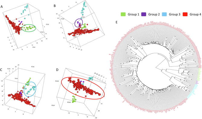
Interactive display of population structure and kinship cladogram. Population structure is displayed as an interactive 3D plot. Users can adjust the display at any angle (e.g., A to D). Individuals are displayed with colors that correspond to the grouping on the kinship cladogram using k-means cluster analysis (E).

Supplementary Figure S6.

Comparison of computing time using four software packages run separately and used within GAPIT. Three standalone software packages are MLMM, FarmCPU, BLINK R version, and BLINK C version. Comparison was performed on differently-sized datasets with respect to duplication of the original data containing 1124 individuals and 12,372 markers (available at http://gscan.well.ox.ac.uk). The duplications were conducted for markers only (A) and individuals only (B).

References

- 1.Wang J., Zhou Z., Zhang Z., Li H., Liu D.i., Zhang Q., et al. Expanding the BLUP alphabet for genomic prediction adaptable to the genetic architectures of complex traits. Heredity (Edinb) 2018;121(6):648–662. doi: 10.1038/s41437-018-0075-0. [DOI] [PMC free article] [PubMed] [Google Scholar]
- 2.Xiao Y., Liu H., Wu L., Warburton M., Yan J. Genome-wide association studies in maize: praise and stargaze. Mol Plant. 2017;10(3):359–374. doi: 10.1016/j.molp.2016.12.008. [DOI] [PubMed] [Google Scholar]
- 3.Pritchard JK, Stephens M, Donnelly P. Inference of population structure using multilocus genotype data. Genetics 2000;155:945–59. [DOI] [PMC free article] [PubMed]
- 4.Pritchard J.K., Stephens M., Rosenberg N.A., Donnelly P. Association mapping in structured populations. Am J Hum Genet. 2000;67(1):170–181. doi: 10.1086/302959. [DOI] [PMC free article] [PubMed] [Google Scholar]
- 5.Zhu X., Li S., Cooper R.S., Elston R.C. A unified association analysis approach for family and unrelated samples correcting for stratification. Am J Hum Genet. 2008;82(2):352–365. doi: 10.1016/j.ajhg.2007.10.009. [DOI] [PMC free article] [PubMed] [Google Scholar]
- 6.Kang H.M., Zaitlen N.A., Wade C.M., Kirby A., Heckerman D., Daly M.J., et al. Efficient control of population structure in model organism association mapping. Genetics. 2008;178(3):1709–1723. doi: 10.1534/genetics.107.080101. [DOI] [PMC free article] [PubMed] [Google Scholar]
- 7.Kang HM, Sul JH, Service SK, Zaitlen NA, Kong SY, Freimer NB, et al. Variance component model to account for sample structure in genome-wide association studies. Nat Genet 2010;42:348–54. [DOI] [PMC free article] [PubMed]
- 8.Zhang Z., Ersoz E., Lai C.-Q., Todhunter R.J., Tiwari H.K., Gore M.A., et al. Mixed linear model approach adapted for genome-wide association studies. Nat Genet. 2010;42(4):355–360. doi: 10.1038/ng.546. [DOI] [PMC free article] [PubMed] [Google Scholar]
- 9.Lippert C., Listgarten J., Liu Y., Kadie C.M., Davidson R.I., Heckerman D. FaST linear mixed models for genome-wide association studies. Nat Methods. 2011;8(10):833–835. doi: 10.1038/nmeth.1681. [DOI] [PubMed] [Google Scholar]
- 10.Svishcheva G.R., Axenovich T.I., Belonogova N.M., van Duijn C.M., Aulchenko Y.S. Rapid variance components–based method for whole-genome association analysis. Nat Genet. 2012;44(10):1166–1170. doi: 10.1038/ng.2410. [DOI] [PubMed] [Google Scholar]
- 11.Li M., Liu X., Bradbury P., Yu J., Zhang Y.-M., Todhunter R.J., et al. Enrichment of statistical power for genome-wide association studies. BMC Biol. 2014;12(1) doi: 10.1186/s12915-014-0073-5. [DOI] [PMC free article] [PubMed] [Google Scholar]
- 12.Wang Q., Tian F., Pan Y., Buckler E.S., Zhang Z., Li Y. A SUPER powerful method for genome wide association study. PLoS One. 2014;9(9):e107684. doi: 10.1371/journal.pone.0107684. [DOI] [PMC free article] [PubMed] [Google Scholar]
- 13.Wells C.R. SAS for mixed models: introduction and basic applications. Am Stat. 2021;75(2):231. [Google Scholar]
- 14.Buckler E.S., Holland J.B., Bradbury P.J., Acharya C.B., Brown P.J., Browne C., et al. The genetic architecture of maize flowering time. Science. 2009;325(5941):714–718. doi: 10.1126/science.1174276. [DOI] [PubMed] [Google Scholar]
- 15.Segura V., Vilhjálmsson B.J., Platt A., Korte A., Seren Ü., Long Q., et al. An efficient multi-locus mixed-model approach for genome-wide association studies in structured populations. Nat Genet. 2012;44(7):825–830. doi: 10.1038/ng.2314. [DOI] [PMC free article] [PubMed] [Google Scholar]
- 16.Liu X., Huang M., Fan B., Buckler E.S., Zhang Z., Listgarten J. Iterative usage of fixed and random effect models for powerful and efficient genome-wide association studies. PLoS Genet. 2016;12(2):e1005767. doi: 10.1371/journal.pgen.1005767. [DOI] [PMC free article] [PubMed] [Google Scholar]
- 17.Huang M., Liu X., Zhou Y., Summers R.M., Zhang Z. BLINK: a package for the next level of genome-wide association studies with both individuals and markers in the millions. GigaScience. 2018;91:399–404. doi: 10.1093/gigascience/giy154. [DOI] [PMC free article] [PubMed] [Google Scholar]
- 18.Bernardo R. Prediction of maize single-cross performance using RFLPs and information from related hybrids. Crop Sci. 1994;34(1):20–25. [Google Scholar]
- 19.VanRaden P.M. Efficient methods to compute genomic predictions. J Dairy Sci. 2008;91(11):4414–4423. doi: 10.3168/jds.2007-0980. [DOI] [PubMed] [Google Scholar]
- 20.Zhang Z, Todhunter RJ, Buckler ES, Van Vleck LD. Technical note: use of marker-based relationships with multiple-trait derivative-free restricted maximal likelihood. J Anim Sci 2007;85:881–5. [DOI] [PubMed]
- 21.Meuwissen THE, Hayes BJ, Goddard ME. Prediction of total genetic value using genome-wide dense marker maps. Genetics 2001;157:1819–29. [DOI] [PMC free article] [PubMed]
- 22.Endelman J.B. Ridge regression and other Kernels for genomic selection with R package rrBLUP. Plant Genome J. 2011;4(3):250–255. [Google Scholar]
- 23.Purcell S., Neale B., Todd-Brown K., Thomas L., Ferreira M.A.R., Bender D., et al. PLINK: a tool set for whole-genome association and population-based linkage analyses. Am J Hum Genet. 2007;81(3):559–575. doi: 10.1086/519795. [DOI] [PMC free article] [PubMed] [Google Scholar]
- 24.Bradbury P.J., Zhang Z., Kroon D.E., Casstevens T.M., Ramdoss Y., Buckler E.S. TASSEL: software for association mapping of complex traits in diverse samples. Bioinformatics. 2007;23(19):2633–2635. doi: 10.1093/bioinformatics/btm308. [DOI] [PubMed] [Google Scholar]
- 25.Pérez P., de los Campos G Genome-wide regression and prediction with the BGLR statistical package. Genetics. 2014;198:483–495. doi: 10.1534/genetics.114.164442. [DOI] [PMC free article] [PubMed] [Google Scholar]
- 26.Lipka AE, Tian F, Wang Q, Peiffer J, Li M, Bradbury PJ, et al. GAPIT: genome association and prediction integrated tool. Bioinformatics 2012;28:2397–9. [DOI] [PubMed]
- 27.Tang You, Liu Xiaolei, Wang Jiabo, Li Meng, Wang Qishan, Tian Feng, et al. GAPIT version 2: an enhanced integrated tool for genomic association and prediction. Plant Genome. 2016;9(2) doi: 10.3835/plantgenome2015.11.0120. [DOI] [PubMed] [Google Scholar]
- 28.Habier D., Fernando R.L., Kizilkaya K., Garrick D.J. Extension of the bayesian alphabet for genomic selection. BMC Bioinf. 2011;12:1–12. doi: 10.1186/1471-2105-12-186. [DOI] [PMC free article] [PubMed] [Google Scholar]
- 29.Yu Jianming, Pressoir Gael, Briggs William H, Vroh Bi Irie, Yamasaki Masanori, Doebley John F, et al. A unified mixed-model method for association mapping that accounts for multiple levels of relatedness. Nat Genet. 2006;38(2):203–208. doi: 10.1038/ng1702. [DOI] [PubMed] [Google Scholar]
- 30.Listgarten Jennifer, Lippert Christoph, Heckerman David. FaST-LMM-Select for addressing confounding from spatial structure and rare variants. Nat Genet. 2013;45(5):470–471. doi: 10.1038/ng.2620. [DOI] [PubMed] [Google Scholar]
- 31.Wang Maggie Haitian, Cordell Heather J., Van Steen Kristel. Statistical methods for genome-wide association studies. Semin Cancer Biol. 2019;55:53–60. doi: 10.1016/j.semcancer.2018.04.008. [DOI] [PubMed] [Google Scholar]
- 32.Aulchenko Y.S., Ripke S., Isaacs A., van Duijn C.M. GenABEL: an R library for genome-wide association analysis. Bioinformatics. 2007;23(10):1294–1296. doi: 10.1093/bioinformatics/btm108. [DOI] [PubMed] [Google Scholar]
- 33.Lee DA, Rentzsch R, Oreng C. GeMMA: functional subfamily classification within superfamilies of predicted protein structural domains. Nucleic Acids Res 2009;38:720–37. [DOI] [PMC free article] [PubMed]
- 34.Knab A.M., Nieman D.C., Sha W., Broman-Fulks J.J., Canu W.H. Exercise frequency is related to psychopathology but not neurocognitive function. Med Sci Sports Exerc. 2012;44:1395–1400. doi: 10.1249/MSS.0b013e31824795f4. [DOI] [PubMed] [Google Scholar]
- 35.Chen C.J., Zhang Z. iPat: intelligent prediction and association tool for genomic research. Bioinformatics. 2018;34:1925–1927. doi: 10.1093/bioinformatics/bty015. [DOI] [PubMed] [Google Scholar]