Mapping Heterogenous Anisotropic Tissue Mechanical Properties with Transverse Isotropic Nonlinear Inversion MR Elastography

Abstract

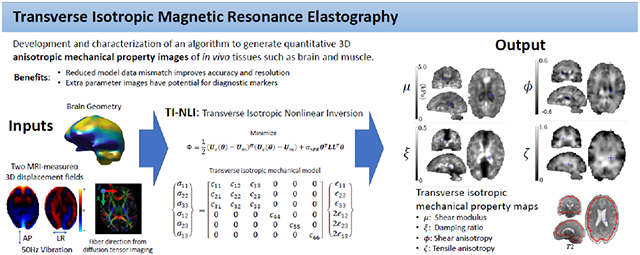
The white matter tracts of brain tissue consist of highly-aligned, myelinated fibers; white matter is structurally anisotropic and is expected to exhibit anisotropic mechanical behavior. In vivo mechanical properties of tissue can be imaged using magnetic resonance elastography (MRE). MRE can detect and monitor natural and disease processes that affect tissue structure; however, most MRE inversion algorithms assume locally homogenous properties and/or isotropic behavior, which can cause artifacts in white matter regions. A heterogeneous, model-based transverse isotropic implementation of a subzone-based nonlinear inversion (TI-NLI) is demonstrated. TI-NLI reconstructs accurate maps of the shear modulus, damping ratio, shear anisotropy, and tensile anisotropy of in vivo brain tissue using standard MRE motion measurements and fiber directions estimated from diffusion tensor imaging (DTI). TI-NLI accuracy was investigated with using synthetic data in both controlled and realistic settings: excellent quantitative and spatial accuracy was observed and cross-talk between estimated parameters was minimal. Ten repeated, in vivo, MRE scans acquired from a healthy subject were co-registered to demonstrate repeatability of the technique. Good resolution of anatomical structures and bilateral symmetry were evident in MRE images of all mechanical property types. Repeatability was similar to isotropic MRE methods and well within the limits required for clinical success. TI-NLI MRE is a promising new technique for clinical research into anisotropic tissues such as the brain and muscle.

GraphicalAbstract

1: Introduction

Magnetic resonance elastography (MRE) generates images of the mechanical properties of tissue using displacement fields measured with phase contrast MRI(Manduca et al., 2001; Muthupillai et al., 1995). MRE methods commonly use mechanical models with assumptions of local homogeneity and isotropy to simplify the associated processing. These approximations are reasonable in large, relatively homogenous organs that also exhibit near-isotropic mechanical behavior, such as liver. Liver MRE has been clinically successful, and is beginning to replace biopsy as the gold standard for diagnosis and staging of fibrosis(Asbach et al., 2008; Hoodeshenas et al., 2018; Huwart et al., 2007; Kennedy et al., 2018; Yin et al., 2007). In this clinical application, artifacts arising from modeling homogeneity and isotropy were minor and less consequential for evaluating liver disease because of its high contrast relative to healthy tissue.

Brain MRE is of growing clinical interest. Decreases in average brain stiffness have been reported in normal aging (Hiscox et al., 2018; Sack et al., 2009) and in neurological conditions such as Alzheimer’s disease (Hiscox et al., 2020; Murphy et al., 2012, 2011), multiple sclerosis (Sandroff et al., 2017; Streitberger et al., 2012; Wuerfel et al., 2010), hydrocephalus (Solamen et al., 2021; Streitberger et al., 2010), amyotrophic lateral sclerosis (Romano et al. 2014), and cerebral palsy (Chaze et al., 2019; McIlvain et al., 2020). Direct inversion techniques assuming local homogeneity have reported region-specific changes in specific cerebral lobes of Alzheimer’s patients(ElSheikh et al., 2017; Murphy et al., 2013, 2011); however, the brain is mechanically heterogeneous being comprised of many subregions with contrast in mechanical properties, and areas of mechanical property gradients cause artifacts in recovered property maps (McGarry et al. 2020). Assuming tissue property homogeneity leads to substantial errors in spatial accuracy, even with idealized simulated data (Barnhill et al., 2019; McGrath et al., 2016). Heterogenous, model-based inversions such as nonlinear inversion (NLI) (McGarry et al., 2013, 2012; Van Houten et al., 2011, 2001, 2000) account for wave reflections and refractions, and high spatial accuracy has been reported in simulation(McGarry et al., 2020) and experimental phantom studies (Solamen et al., 2018), leading to reliable localized property estimates in brain structures such as the hippocampus (Daugherty et al., 2020; Delgorio et al., 2021) and corpus callosum(Johnson et al., 2013). Reducing artifacts which arise from model-data mismatch is vital to improving the sensitivity of MRE in brain applications, which is essential for revealing recent observations of relationships between cognitive function and the mechanical properties of the contributing structures (L. V. Hiscox et al., 2020; Johnson et al., 2018; Schwarb et al., 2019, 2016).

In this study we extend the NLI approach to incorporate tissue anisotropy as well as heterogeneity. Certain brain regions contain aligned axons that makeup fiber bundles which carry and distribute neuronal signals between regions. Stiffness along these tracts is likely higher than in transverse directions, and accordingly, violates isotropic assumptions and causes wavefield-dependent artifacts when isotropic MRE is applied to anisotropic tissue (Anderson et al., 2016; McGarry et al., 2020). The need to account for both heterogeneity and anisotropy in a single inversion approach motivates development of transverse isotropic nonlinear inversion (TI-NLI). This algorithm adopts a previously-reported nearly incompressible transverse isotropic (NITI) finite element model (McGarry et al., 2020), and incorporates it into a subzone-based heterogenous nonlinear inversion MRE property reconstruction algorithm.

Anisotropic MRE inversions have been presented previously by Sinkus (Sinkus et al., 2005), Qin et al (Green et al., 2013; Qin et al., 2012), Miller (Miller et al., 2018a), and Romano (Romano et al., 2012). Promising clinical results have been published with the Romano waveguide algorithm (Mazumder et al., 2015; Romano et al., 2014); however, evaluation of its predictions by comparison to simulated or experimental phantom data has been limited. These tests are needed as effects of disease on the input DTI parameters for the waveguide inversion may be predictive, without the added value of an anisotropic mechanical model. The direct inversion algorithm of Qin et al. was convincingly validated in a phantom system, though it does not appear to have been implemented for in vivo brain studies. In brain, property image artifacts would be likely in regions of mechanical property gradients because of the local homogeneity assumption. The virtual fields method of Miller reconstructs a homogeneous set of transverse isotropic properties and was characterized in a simulated cardiac model and an isotropic phantom (Miller et al., 2018b, 2015); however, to our knowledge the method has not been used with in vivo data. This homogeneous implementation will have limited use in brain as substantial spatial variation in mechanical properties is expected; however, the virtual fields method could be adapted to support heterogenous properties. Recently, a finite element-based method has been presented by Babaei (Babaei et al., 2021) which can recover heterogeneous distributions of shear moduli parallel and perpendicular to the fiber directions and was comprehensively evaluated in silico and demonstrated in vivo. Tensile anisotropy was not accounted for in this model, so it cannot recreate the fast and slow shear waves predicted and detected in transverse isotropic materials (Feng et al., 2013; Schmidt et al., 2016).

An additional benefit of anisotropic MRE is the ability to assess a wider range of material property parameters, which may inform clinical diagnoses of neurodegenerative conditions. Disease-related biological processes may affect these anisotropic parameters, differently and with more sensitivity, compared to averaged stiffness recovered through isotropic inversion. Thus, these newly estimated anisotropic mechanical property parameters may improve differential diagnoses as most brain diseases have a non-specific softening effect, which is similar to normal aging processes, and likely to confound the diagnostic signatures that may be available with MRE, if its sensitivity can be increased substantially through recovery of anisotropic mechanical property parameters.

2: Methods

2.1: Nearly incompressible transverse isotropic (NITI) model

The constitutive equation in Voigt notation (6x1 vector representation of the 2^nd order tensors) for the relationship between the stress, {σ}, and strain, {ϵ}, in a nearly incompressible transverse isotropic (NITI) material (Feng et al., 2013; Schmidt et al., 2018, 2016; Tweten et al., 2015) in a coordinate system aligned with the axis of symmetry, takes the form

$$\left\{\begin{array}{c}\hfill {\sigma }_{11}\hfill \\ \hfill {\sigma }_{22}\hfill \\ \hfill {\sigma }_{33}\hfill \\ \hfill {\sigma }_{12}\hfill \\ \hfill {\sigma }_{23}\hfill \\ \hfill {\sigma }_{13}\hfill \end{array}\right\}=\left[\begin{array}{cccccc}\hfill c_{11}\hfill & \hfill c_{12}\hfill & \hfill c_{13}\hfill & \hfill 0\hfill & \hfill 0\hfill & \hfill 0\hfill \\ \hfill c_{21}\hfill & \hfill c_{22}\hfill & \hfill c_{23}\hfill & \hfill 0\hfill & \hfill 0\hfill & \hfill 0\hfill \\ \hfill c_{31}\hfill & \hfill c_{32}\hfill & \hfill c_{33}\hfill & \hfill 0\hfill & \hfill 0\hfill & \hfill 0\hfill \\ \hfill 0\hfill & \hfill 0\hfill & \hfill 0\hfill & \hfill c_{44}\hfill & \hfill 0\hfill & \hfill 0\hfill \\ \hfill 0\hfill & \hfill 0\hfill & \hfill 0\hfill & \hfill 0\hfill & \hfill c_{55}\hfill & \hfill 0\hfill \\ \hfill 0\hfill & \hfill 0\hfill & \hfill 0\hfill & \hfill 0\hfill & \hfill 0\hfill & \hfill c_{66}\hfill \end{array}\right]\left\{\begin{array}{c}\hfill {ϵ}_{11}\hfill \\ \hfill {ϵ}_{22}\hfill \\ \hfill {ϵ}_{33}\hfill \\ \hfill 2{ϵ}_{12}\hfill \\ \hfill 2{ϵ}_{23}\hfill \\ \hfill 2{ϵ}_{13}\hfill \end{array}\right\}.$$ (1)

Defining the fiber axis as the x₁ direction, the components of the 6x6 elasticity matrix, [C], are given by

$$\begin{gathered} c_{11}=\kappa +\frac{4}{3}\mu \left(1+\frac{4}{3}\zeta \right),c_{22}=c_{33}=\kappa +\frac{4}{3}\mu \left(1+\frac{1}{3}\zeta \right),c_{44}=c_{66}=\mu (1+\varphi ), \\ {c}_{12}=c_{13}=c_{21}=c_{31}=\kappa -\frac{2}{3}\mu \left(1+\frac{4}{3}\zeta \right),c_{32}=c_{23}=\kappa -\frac{2}{3}\mu \left(1-\frac{2}{3}\zeta \right),c_{55}=\mu \end{gathered}$$ (2)

Here, μ is the shear modulus in the plane normal to the fiber axis, ϕ is the shear anisotropy, ζ is the tensile anisotropy, and κ is the isotropic bulk modulus. This form has advantages for inversion with an isotropic damping assumption, since μ can be complex-valued while ϕ and ζ can be real-valued. The isotropic damping ratio in this case is defined as $\xi =\frac{Im(\mu )}{2Re(\mu )}$. Alternatively, ϕ and ζ could be complex-valued for anisotropic damping; however, applying parameter bounds to ensure physically realistic positive moduli in all directions and interpreting the complex-valued μ and ζ becomes difficult. This paper uses the isotropic damping form where the damping ratio is independent of direction. Equations 1 and 2 are applied as constitutive equations in the steady-state time-harmonic Navier’s equation,

$$\nabla \cdot \sigma =-\rho {\omega }^2\mathit{U},$$ (3)

to compute complex-valued displacement amplitudes, U, at harmonic frequency, ω, using the finite element method. ρ is the material density, and σ is the rank 2 stress tensor where the components are defined through Equations 1 and 2, with the definition of the strain tensor ${ϵ}_{ij}=\frac{1}{2}\left(\frac{\partial U_i}{d{x}_j}+\frac{\partial U_j}{\partial x_i}\right)$. Fiber directions are determined a priori (in vivo cases use the primary diffusion direction from diffusion tensor imaging). Finite element implementation of the heterogeneous NITI model has been described in more detail in a previous publication(McGarry et al., 2020).

Waves resulting from deformation of a NITI material can be classified into three types – a very fast longitudinal wave with speed c_l, and “slow” (or “pure shear”) and “fast” (or “quasi-shear”) shear waves with speeds c_slow and c_fast, given by(Tweten et al., 2015)

$$c_l=\sqrt{\frac{\kappa +2\mu }{\rho }},c_{slow}=\sqrt{\frac{\mu (1+\varphi co{s}^2\theta )}{\rho }},c_{fast}=\sqrt{\frac{\mu (1+\varphi co{s}^{2}2\theta +\zeta si{n}^{2}2\theta )}{\rho }}$$ (4)

For nearly incompressible soft tissues, typical values are c_l ≈ 1500ms⁻¹ and c_slow∣fast ≈ 1 − 10m s⁻¹. These formulas are valid for undamped materials with real-valued stiffnesses; viscoelasticity will increase propagation speed (Guidetti and Royston, 2018).

2.2: Transverse isotropic nonlinear inversion (TI-NLI) algorithm

The forward NITI model was implemented in a subzone-based NLI algorithm (Doyley et al., 2004; Van Houten et al., 2001). MRE measurements are full-volume, 3D vector fields of the complex-valued displacement amplitude during steady-state vibration. NLI minimizes Φ as the difference between the measured MRE displacement field, U_m, and a computational model, U_c(θ),

$$\Phi =\frac{1}{2}({\mathit{U}}_c(\theta )-{\mathit{U}}_m{)}^H({\mathit{U}}_c(\theta )-{\mathit{U}}_m)+{\alpha }_{SPR}{\theta }^T\mathit{L}{\mathit{L}}^T\theta$$ (5)

through iteratively updating a parameterized description of the spatially varying unknown mechanical properties, θ, using gradient descent methods. The superscript H denotes the conjugate transpose (Hermitian) of the 3Nx1 U vectors containing the x, y, and z components of the displacement amplitudes at each of N measurement points. Soft prior regularization (SPR) promotes homogeneity within predefined regions, and can be implemented by setting α_SPR > 0 with prior spatial information (usually generated through atlas-based segmentation of anatomical images) to compute the L matrix (McGarry et al., 2013). No prefiltering of the input displacement data is required.

Boundary conditions required for computing U_c(θ) are fixed displacement conditions taken from the MRE measurements. The subzone method takes advantage of full-volume displacement data to reduce the heavy computational load of iterative solution strategies by dividing the domain into a set of overlapping cubic subzones. Zones are processed in parallel on a distributed computing cluster, then the global property solution is assembled from the union of subzone solutions. Inversions are not sensitive to subzone size within a range of 0.64-1.0 shear wavelengths per zone (Anderson et al., 2017; Solamen et al., 2018). In this study we used 25 mm cubic zones, which falls in the middle of this range and is consistent with all 50 Hz brain MRE studies performed with NLI to date. The subzone process is repeated for a number of global iterations with randomly generated sets of subzones until the property estimates stabilize. A Gaussian smoothing (1.5 mm kernel width) is applied at each global iteration to stabilize property estimates. When SPR is active, smoothing across region boundaries is reduced by 50% to improve contrast recovery while maintaining stability through the combined influence of SPR and Gaussian smoothing. Generally, smaller numbers of gradient descent iterations per subzone (2-4) and more global iterations (approximately 100) is more efficient and stable relative to enforcement of full convergence of the minimization problem on every subzone with smaller numbers of global iterations.

Unknown mechanical property fields are supported nodally on independent 8-node hexahedral finite element meshes to allow the density of unknown properties to be controlled independently of data resolution and the resolution of the 27-node quadratic hexahedral finite element mesh used to compute U_c (McGarry et al., 2012). Previous implementations of NLI with isotropic models recover only the isotropic real and imaginary shear modulus, which converges with property mesh resolution equal to the data resolution. In the NITI model, the inversion has lower sensitivity to anisotropy parameters, ϕ and ζ, which leads to much slower convergence. The lower sensitivity was mitigated by using a coarser resolution for ϕ and ζ in early global iterations (10 mm for iterations 1-10, 4 mm for iterations 10-50, and 2 mm for the final 50 iterations). Resolution of the real and imaginary parts of μ remains at 2 mm for the entire inversion. A more sophisticated L-BFGS-B quasi-Newton (QN) gradient descent algorithm (Byrd et al., 1995; Zhu et al., 1997) with a secant method linesearch is used rather than the conjugate gradient method from earlier NLI implementations; 2 QN and 2 linesearch iterations are used for iterations 1-10, 3 QN and 3 linesearch iterations for iterations 11-50, and 4 QN and 3 linesearch iterations for the final 50 iterations are used. Lower bounds of μ > 200Pa, and ϕ, z > −1 were enforced to ensure positive moduli and realistic free energy. These parameters were selected to balance convergence speed, contrast recovery, and sensitivity to noise or artifacts; the same parameters were used for all NITI inversions shown in this paper.

2.3: Gradient calculation

Iterative minimization requires computation of the gradient of the error function in parameter space, $\frac{\partial \Phi }{\partial \theta }$. This term is computed efficiently through the adjoint method, which requires one factorization of the forward finite element stiffness matrix and two back-substitutions to compute the full $\frac{\partial \Phi }{\partial \theta }$ vector. The method is described in the literature (Tan et al., 2017). Briefly, two solutions of the forward model are computed with the current θ estimate: U_c using the forcing vector from the standard forward problem, and U_a using the displacement error, (U_c(θ) − U_m), as the forcing vector. The terms of the gradient are then computed using

$$\frac{\partial \Phi }{\partial {\theta }_i}={\mathit{U}}_a^T\frac{\partial \mathit{A}}{\partial {\theta }_i}{\mathit{U}}_{\mathit{c}}$$ (5)

$\frac{\partial \mathit{A}}{\partial {\theta }_i}$ is the forward finite element stiffness matrix differentiated with respect to the i^th mechanical property parameter represented in θ. The simple form of Equations 1 and 2 make differentiation trivial – for example, $\frac{\partial \mathit{A}}{\partial \mu }$ is built with the same assembly process as the forward problem (McGarry et al., 2020) where $\frac{\partial \mathit{C}}{d\mu }$ replaces C. $\frac{\partial \mathit{A}}{\partial {\theta }_i}$ is extremely sparsely populated as each θ_i has a limited area of influence, which makes the computational cost of the gradient assembly much lower than the matrix factorization of the forward problem. Finite difference checks of the gradient terms match those computed with the adjoint method to 5 significant figures.

2.4: Simulated displacement data

Two idealized, simulated geometries were created to test the behavior of anisotropic MRE under tightly controlled conditions. Both geometries represented a 90 mm cube, and are illustrated in Figure 1. Geometry 1 has an isotropic background with four cubic, 20 mm inclusions. Fibers in each of the four inclusions were oriented in the x, y, z directions, and at an angle across the main diagonal of the cubic inclusion, respectively. Geometry 2 has an isotropic background with a spherical anisotropic shell of outer diameter 80 mm and inner diameter 60 mm, resulting in a shell thickness of 10 mm. Fiber directions within the shell followed the longitudinal lines of the spherical geometry which gives all possible fiber orientations in this simulated geometry. Nine different fixed displacement amplitude boundary conditions were applied to each geometry to generate nine different displacement fields: each of the x, y, z = 0 faces, with displacements applied in the x, y and z directions, giving 6 shear actuations and 3 compressive actuations from which to choose. Typical examples of these displacements are given in Figure 1. Simulated displacements were computed on a 1.5 mm resolution mesh of 27-node quadratic hexahedral finite elements with a total of 226981 nodes. These displacements were interpolated using cubic splines to the approximate resolution of MRI measurements, 2.0455 mm to represent the MRI measurement data and avoid the ‘inverse crime’ of running the forward and inverse problems on an identical mesh. Fiber directions were sampled at the MRI resolution using the ideal geometries of the shell and cubic inclusions as an approximation of finite resolution measurements of the true fiber directions with DTI. The effect of noise in the fiber direction estimates was tested by adding a randomly oriented vector with Gaussian distributed length (mean=0, standard deviation equal to a given percentage of the normalized vector length) to the normalized ideal fiber direction, followed by renormalization. Prescribed fiber directions in isotropic regions were assigned to be pure noise, as would be the output DTI measures in regions that do not have a preferred fiber direction. Single-direction inversions for three different displacement fields were investigated for Geometry 1 to represent a range of propagation and polarization directions (boundary conditions: x = 0 face with y-directed shear motion, z = 0 face with x-directed shear motion, and z = 0 face with z-directed compressive motion). TI-NLI inversions of Geometry 2 were performed using two arbitrarily chosen displacement fields: boundary conditions: z = 0 face with x-directed shear motion, and the y = 0 face with y-directed compressive motion. Only two of the 9 available displacement fields were used to approximate the two vibration directions (AP and LR) currently achieved in brain MRE experimentally (Smith et al., 2020).

Figure 1:

Illustration of simulated cubic phantom geometries, and a rendering of typical harmonic vibration displacement fields resulting from shear (top) and compressive (bottom) boundary conditions.

A previously published full brain MRE simulation (McGarry et al., 2020) was used to generate realistic synthetic MRE data to evaluate the accuracy of the NITI inversion in cases with known and controllable anisotropy. The simulated NITI brain model was built from a clinical brain MRE examination with T2-weighted anatomical images and atlas-based segmentations of white matter tracts and subcortical gray matter structures. MRE displacement data at 50 Hz was used to simulate wave fields with actuation of the head in the anterior posterior (AP), and left-right (LR) directions, and DTI images of the fractional anisotropy and primary eigenvector of the diffusion tensor were used to calculate fiber direction. A full-brain finite element geometry was generated from one of the anatomical brain images, with fiber directions assigned from the primary diffusion eigenvalue of the DTI data. Each of 10 white matter tracts and 6 subcortical gray matter structures were assigned shear moduli based on the literature if available (Johnson et al., 2016), or unpublished isotropic MRE analyses. ϕ and ζ were assigned based on the local fractional anisotropy measure through DTI. A random multiplier between 0.9 and 1.1 was applied to ensure ϕ ≠ ζ. The assigned properties are tabulated in a previous publication (McGarry et al., 2020). Boundary conditions for AP and LR vibration of the skull were taken from the two MRE displacement datasets on the brain surface to ensure realistic wavefields. Simulated Gaussian noise with zero mean and standard deviation equal to a percentage of the global mean displacement amplitude at t = 0 and $t=\frac{\pi }{4}$ in the harmonic cycle was added in some cases. The effective octahedral shear strain SNR (OSS-SNR) (McGarry et al., 2011) was estimated for each noisy field using a central difference approximation to compare to in vivo data.

2.5: Experiments with simulated data

Isotropic inversions of the cube geometry were performed to demonstrate dependence of commonly used MRE inversions on wave propagation, wave polarization, and fiber orientation angles in anisotropic materials. Wave propagation in the brain is difficult to control in vivo due to the skull so wavefield dependence is an undesirable behavior. To interpret results obtained from isotropic inversion of intentionally anisotropic data, the primary propagation direction for each displacement set was computed using the method described by (Okamoto et al., 2019), and an approximation of the effective isotropic stiffness for each case was derived using the wave propagation speeds in Equation 4,

$${\mu }_{eff}=\frac{\mid \overrightarrow{u}\cdot {\overrightarrow{m}}_s\mid }{(\mid \overrightarrow{u}\cdot {\overrightarrow{m}}_s\mid +\mid \overrightarrow{u}\cdot {\overrightarrow{m}}_f\mid )}{\mu }_{slow}+\frac{\mid \overrightarrow{u}\cdot {\overrightarrow{m}}_f\mid }{(\mid \overrightarrow{u}\cdot {\overrightarrow{m}}_s\mid +\mid \overrightarrow{u}\cdot {\overrightarrow{m}}_f\mid )}{\mu }_{fast},$$ (6)

where μ_slow = μ(1 + ϕcos² θ) and μ_fast = μ(1 + ϕ cos² 2θ + ζ sin² 2θ), $\overrightarrow{u}$ is the displacement vector, and the slow and fast shear wave polarization directions are given by ${\overrightarrow{m}}_s=\overrightarrow{a}\times \overrightarrow{n}$ and ${\overrightarrow{m}}_f={\overrightarrow{m}}_s\times \overrightarrow{n}$, respectively, for fiber direction vector $\overrightarrow{a}$ and propagation direction $\overrightarrow{n}$, with θ = cos⁻¹($\overrightarrow{n}\cdot \overrightarrow{a}$). Both m_f and m_f are normalized to length 1. Note that μ_eff is an approximation based on understanding of the anisotropic material structure and computed wave field. The actual isotropic μ value recovered by an isotropic inversion will depend on many factors not captured in this estimate.

2.6: In vivo brain imaging protocol

Two sets of MRE displacements were acquired sequentially for each imaging session: one with vibration in the LR direction and one in the AP direction (Anderson et al., 2016; Smith et al., 2020). Vibrations were applied at 50 Hz using the Resoundant pneumatic actuator system with the passive pillow driver for AP actuation and a custom lateral driver attached to the head coil for LR actuation (Caban-Rivera et al., 2021). MRE data were acquired using a 3D multiband, multishot spiral sequence with 2.0 mm isotropic resolution and parameters including: 240 mm field-of-view; 120x120 matrix; 64 slices; TR/TE = 2240/76 ms. DTI data was also acquired at 1.5 mm (210 mm field-of-view; 140x140 matrix; 92 slices; TR/TE = 3520/95.2 ms; 137 directions; b = 1500 and 3000 s/mm²) and co-registered to MRE data to provide fiber directions and fractional anisotropy (FA) maps. Repeatability was investigated by collecting ten independent datasets on the same subject (M, 23 y) who provided written, informed consent for this study approved by the Institutional Review Board. OSS-SNR for these data ranged from 3.5-18.8, with mean 10.2 and standard deviation 4.5.

2.7: In vivo data processing

Inversions using the NITI model with the same parameters as the simulated datasets, described above, were applied to the ten repeated in vivo brain datasets. Both AP and LR displacement sets were used in the objective function to recover a single set of NITI parameters. Mean and variance images for each NITI property were computed by six degree-of-freedom rigid body registration of all datasets to the first dataset using FSL FLIRT (Jenkinson et al., 2012, 2002). Inversion time with two displacement sets for a full brain at 2mm resolution using 64 cores of Dartmouth’s Discovery computing cluster (Dartmouth RC, 2022) ranged from 12 to 20 hours.

3: Results

Figure 2 presents isotropic inversions of anisotropic data in a system where the propagation and polarization directions of the shear waves are controlled by actuation of one face of a cube, and illustrates the artifacts arising from this model-data mismatch. The effective isotropic stiffness estimate, μ_eff, generated a priori from maps of the wave polarization and propagation directions, fiber direction, and simulated anisotropic properties can predict when an inclusion ‘disappears’ from the isotropic inversion for a given wavefield.

Figure 2:

Isotropic inversion of simulated data with three different displacement boundary conditions. The phantom had cubic inclusions with nonzero values of either ϕ = 0.5 (left column) or ζ = 0.5 (right column), with 4 different fiber orientations: one in each of the 3 coordinate directions and in the (1,1,1) direction across the diagonals of the cube. The effective isotropic stiffness, μ_eff, estimated from the fiber direction and wave propagation and polarization directions is compared to the isotropic μ estimates from applying an isotropic NLI MRE algorithm to the anisotropic simulated data. Whether an anisotropic inclusion is visible in an isotropic inversion is predictably dependent on the propagation and polarization directions of the displacement field. For the ζ = 0.5 case, inclusions with fibers aligned with coordinate axes are not visible in most cases as sin(2θ) = 0 in Equation 4.

Figure 3 presents TI-NLI inversions from the shell simulation and demonstrates that the algorithm recovers contrast in μ, ϕ, and ζ accurately from two independent displacement fields with minimal cross-talk between parameter types. Similarly, the brain simulation in Figure 4 demonstrates accurate recovery of the prescribed NITI parameter images of brain structures from simulated displacement fields which mimic AP and LR-directed actuations of the head that occur in an in vivo MRE exam. Realistic levels of simulated measurement noise affected the ϕ and ζ anisotropy images more than the Re(μ) and ξ maps; however, reasonable quantitative values and spatial accuracy were maintained in all parameters.

Figure 3:

TI-NLI of simulated data using two displacement fields. One plane through the center of the shell is shown: each column shows an inversion of simulated data with contrast in only one of the three stiffness parameters. Contrast in each of the parameters is recovered with minimal cross-talk in the other parameters. Incomplete contrast recovery (due to regularization) is evident, and the ϕ and ζ fields have minor spatial artifacts from low sensitivity in some regions due to the idealized geometry and boundary conditions.

Figure 4:

Noise in DTI directions does not have a large effect on recovered properties. A 3D vector plot of each noise level applied to an x-directed field is shown in the top row, and a slice in the xz plane of the shell phantom is shown in the lower rows. This example has contrast in both ϕ and ζ. The plots in the rightmost column show the recovered mean and standard deviation of the background and inclusion over the full volume and with a larger range of noise levels than the single slice images in the center 3 columns. Results are similar for contrast in ϕ or ζ alone. TI-NLI inversions of isotropic inclusions with contrast in μ only are unaffected by noise in the DTI directions.

Figure 4 shows results from the shell simulation of Figure 3 with different levels of noise added to the fiber direction map used in the inversion to mimic noise in the DTI-derived fiber orientations. DTI noise had minimal effect on the recovered images. Only small decreases in anisotropy estimates occurred at very high noise levels, and ϕ ≈ ζ ≈ 0 was recovered in isotropic regions with completely random fiber directions.

Figure 6 presents in vivo TI-NLI inversions. Results from a single imaging session, along with voxel-by-voxel mean and standard deviation over ten repeated, co-registered TI-NLI MRE exams are given. Resolution of shear modulus and damping ratio was improved compared to previously published isotropic inversions (Johnson et al., 2013; Hiscox et al., 2020; McGarry et al., 2020), and anisotropy images show bilateral symmetry and anatomical structure. Interestingly, the shear anisotropy, ϕ, has both positive and negative values whereas the tensile anisotropy, ζ, is nearly all positive and approximately 2x higher than ϕ, with isolated small negative values around the boundary.

Figure 6:

In vivo TI-NLI property images from a single scan, and voxel-by-voxel mean and standard deviation for 10 repeated in vivo MRE exams of the same subject. Repeat scans were aligned using a 6 DOF rigid body registration of the anatomical T2 images. Blue crosses show locations of the other orthogonal image display planes.

4: Discussion

In this study, we implement a transverse isotropic nonlinear inversion (TI-NLI) algorithm and demonstrate its performance in recovering anisotropic mechanical properties in white matter tracts from two displacement fields collected with multi-excitation MRE. The nearly incompressible transverse isotropic (NITI) model for MRE proposed by Tweten et al. (Feng et al., 2013; Tweten et al., 2015) is incorporated into a subzone-based nonlinear inversion algorithm. The resulting approach handles heterogeneity in both properties and fiber direction, which are present in the brain. Use of more than one displacement field is important to probe directional dependence; with two displacement fields, computational time is increased by an extra back-substitution compared to isotropic inversion involving a single displacement field.

The recovered TI-NLI property maps have better effective resolution than property maps from previous isotropic NLI images for several reasons. With two input displacement sets, more data are available for use in inversion. Furthermore, those data are of a higher quality than in previous studies, largely because of MRI sequence improvements since the default isotropic NLI inversion parameters were set – these have remained unchanged over the last 8 years in the interest of maintaining a consistent inversion protocol. The inclusion of extra parameters in the NITI model required updating the gradient descent strategy to Quasi-Newton, optimizing the multi-mesh structure (McGarry et al., 2012), and tuning the update weightings of the different parameter types. The data quality and quantity improvements yielded increased property parameter resolution while maintaining adequate stability with in vivo images. Another factor allowing for better resolution may be reduced model-data mismatch due to accounting for tissue anisotropy correctly. It is evident in Figures 5 and 6 that ϕ and ζ are more sensitive to measurement noise, which is expected as only a portion of the wave energy is in modes with the propagation and polarization directions required for the anisotropy parameters to have an influence on the displacement fields. Data quality requirements to achieve accurate values of anisotropy parameters may be higher than in previous isotropic MRE studies. The inversion parameters used for the method validation presented here will likely be updated in future work when more in vivo data is available as we seek to balance the resolution and stability of the in vivo property maps.

Figure 5:

TI-NLI of simulated brain data: Images of the base storage modulus, Re(μ) (kPa), damping ratio, $\xi =\frac{Im(\mu )}{2Re(\mu )}$, shear anisotropy, ϕ, and tensile anisotropy, ζ. The ground truth properties are compared to recovered properties for noise-free input displacements, and with 3 levels of added Gaussian measurement noise, 1, 2 and 5%. Mean OSS-SNR of the simulated data is indicated to compare with the in vivo data in Figure 6 which had OSS-SNR 10.2±4.5, range [3.5 – 18.8]. Blue crosses on each image show the intersection of the other two orthogonal image display planes.

Incomplete contrast recovery is observed in the simulated data of Figures 3, 4 and 5 which is a result of the regularization levels required to ensure stability with in vivo data. The structures being imaged are sub-wavelength in size and the same inversion parameters are used for all data sources - with ideal simulated data we can tune the inversion parameters by adjusting regularization weights and performing more optimization iterations per subzone to achieve contrast recovery to close to 100%; however, this gives unstable inversions in the presence of measurement noise and model-data mismatch which is unavoidable in the in vivo case.

The TI-NLI inversions are initialized with ϕ = ζ = 0, and no constraints are imposed in the algorithm to preferentially select positive or negative anisotropy (other than enforcing ϕ, ζ > −1 to ensure realistic free energy); thus, the resulting sign of these parameters is determined by the data. The in vivo tensile anisotropy images in Figures 6 are nearly all positive, indicating that stretching along the fibers provides more resistance than stretching across the fibers. Shear anisotropy, however, appears as both positive and negative in recovered property maps – positive ϕ indicates that shear resistance in planes parallel to the fiber direction is higher than in the plane perpendicular to the fiber, whereas negative ϕ indicates that shear resistance is higher in planes perpendicular to the dominant fiber direction.

Brain white matter is a composite material, where major structural components are aligned tracts of myelinated axons supported by softer connective tissues. ζ > 0 would be expected in white matter as the continuous tracts of stiffer myelin must be stretched for tensile deformation to occur along the fibers, whereas across the fibers the softer connective tissue can stretch independently of the stiff myelin. Shear deformation of composite materials is more complicated, and resistance to shear depends on the geometry, stiffness, distribution, and cross-linking, such as may be the case in gray matter. Hence, whether shear anisotropy ϕ should be positive or negative in general is not clear (Holzapfel et al., 2019), even if the modulus of the fiber material is greater. Bilateral symmetry, correspondence with anatomical structure, and repeatability for both ϕ and ζ images give confidence that these parameters represent true features of the brain’s anatomy and microstructure.

Results inside the ventricles in Figure 6 are not considered reliable as a solid model is applied to the fluid spaces. Fluid cannot be adequately modeled as a very soft nearly incompressible solid, as the shear wavelength becomes very small, and the discretization error becomes very large as the number of finite element nodes per wavelength decreases and corrupts the computational model solution. The effects of the ventricles on the surrounding tissue (e.g. wave reflection) can be approximated by soft solid ventricles, which is what the model tends to find. However, it cannot overcome the limits of spatial resolution of the FE model to get to extremely low shear moduli as discretization error swamps the solution, so the actual values in the ventricles cannot be considered accurate for both shear moduli and anisotropies. The ventricles can be removed from the geometry before inversion; however, this does not improve inversion accuracy and is an extra processing step.

The current TI-NLI anisotropic inversion is the first to incorporate material anisotropy for both shear and tensile moduli in an algorithm that also handles heterogeneity. We comprehensively evaluated TI-NLI through comparisons to realistic simulated data and in vivo repeatability. The promising initial results presented here suggest it may be a valuable tool for clinical brain research.

In future work, the TI NLI method may be used to estimate properties in other anisotropic materials, including experimental phantoms and muscle. We will also investigate relationships between the number of displacements fields and the accuracy of TI NLI inversions. Use of two displacement fields is feasible for in vivo brain imaging (Smith et al., 2020) but may not be necessary for accurate reconstruction of TI-NLI parameters in all cases.

5: Conclusions

Transverse isotropic nonlinear inversion MRE is feasible and produces spatially and quantitatively accurate maps of the shear modulus, damping ratio, and shear and tensile anisotropy from simulated data, both with and without added noise. Images of the anisotropic elastic parameters obtained by inverting in vivo human brain data show bilateral symmetry, expected structure and good repeatability. These results establish anisotropic MRE in general, and TI-NLI specifically, as promising tools for characterizing mechanical behavior of the brain.

Highlights.

• A novel finite element based magnetic resonance elastography inversion for in vivo mechanical property imaging of heterogenous, anisotropic tissue is presented.

• Imaged parameters include shear modulus, damping ratio, shear anisotropy and tensile anisotropy.

• Good quantitative and spatial accuracy, as well as low noise sensitivity was demonstrated with simulated data.

• In vivo brain imaging demonstrated bilateral symmetry and correspondence with anatomical structure for all parameters and good scan-to-scan repeatability.

Abbreviations:

MRE

Magnetic Resonance Elastography

NITI

Nearly incompressible transverse isotropic

NLI

Nonlinear inversion

TI-NLI

Transverse isotropic nonlinear inversion

AP

Anterior-posterior

LR

Left-right

DTI

Diffusion tensor imaging

FA

Fractional anisotropy

SPR

Soft prior regularization