Local Sound Speed Estimation for Pulse-Echo Ultrasound in Layered Media

Abstract

Our previous methodology in local sound speed estimation utilized time delays measured by the cross-correlation of delayed full synthetic aperture channel data to estimate the average speed of sound. However, focal distortions in this methodology lead to biased estimates of the average speed of sound, which, in turn, leads to biased estimates of the local speed of sound. Here, we demonstrate the bias in the previous methodology and introduce a coherence-based average sound speed estimator that eliminates this bias and is computationally much cheaper in practice. Because this coherence-based approach estimates the average sound speed in the medium over an equally-spaced grid in depth rather than time, we derive a refined model that relates the local and average speeds of sound as a function of depth in layered media. A fast, closed-form inversion of this model yields highly accurate local sound speed estimates. The root mean-square (RMS) error of local sound speed reconstruction in simulations of two-layer media is 4.6, and 2.5 m/s at 4 and 8 MHz, respectively. This work examines the impact of frequency, f-number, aberration, and reverberation on sound speed estimation. Phantom and in-vivo experiments in rats further validate the coherence-based sound speed estimator.

I. INTRODUCTION

Sound speed plays a fundamental role in the interaction of the ultrasound imaging system with the imaged medium. Sound speed not only affects the time of arrival of an acoustic wave to a particular location in space, but is also partially responsible for impedance changes, which produce the reflections needed for ultrasound imaging, as well as refraction and diffraction effects in spatially-varying media. B-mode ultrasound imaging generally assumes that the speed of sound in a medium is constant, so that reflections due to scattering in the medium can be focused by simply delaying-and-summing according to known geometric distances and the speed of sound. Ideally, if the speed of sound used in beamforming matches the true speed of sound in the medium, the backscattered reflections should be well-aligned after applying delays. However, an error in the speed of sound will result in misalignment of channel signals and thereby degrade imaging performance. Furthermore, if significant sound speed heterogeneity is present in the medium, higher-order phase aberrations can contribute to further signal misalignment after applying geometric delays, and cause degradation of the ultrasound image [1].

Speed of sound can often be a mechanism for tomographic imaging by utilizing the differential times of flight along various paths of propagation [2]–[7]. Many of these tomographic sound speed imaging techniques propose to differentiate diseased tissue from normal tissue by using a through-transmission system [8]–[10], or a reflection-based pulse-echo system [3], [5]. While these reflection-based tomographic approaches can effectively measure lateral variations in the speed of sound, they often have difficulty accurately measuring the average speed of sound or axial variations in a layered medium [11]–[13]. Techniques that utilize direct measurement of the average speed of sound can accurately capture axial variations in local speed of sound in layered media where lateral sound speed variations are negligible [14]–[17]. Transmission-based ultrasound computed tomography [8]–[10] can accurately estimate both lateral and axial variations in the speed of sound because they often provide a complete angular coverage of the medium and enable the k-space coverage necessary for accurately mapping the speed of sound. The main disadvantage of this approach is that it requires through-transmission.

Knowledge of the speed of sound in the medium based on sound speed reconstruction has also been used to perform distributed aberration correction [14], [18]. In addition to image correction, speed of sound can also be used as a biomarker for diseases such as non-alcoholic fatty liver disease (NAFLD) [15], [16]. Fat accumulation in the liver has been shown to significantly decrease the speed of sound. Across the literature, the speed of sound ranges from 1560–1590 m/s in healthy liver and 1510–1530 m/s in fatty liver [19]–[21]. Recent work in pulse-echo ultrasound has focused on estimating the speed of sound in the liver through the abdominal wall, which is well-described by a layered medium [4], [14], [15]. Layered media models have also been used to estimate the speed of sound in the livers of patients in order to diagnose hepatic steatosis [15], [16], [22].

Our previous work [23] utilized residual time delays measured by the cross-correlation of geometrically-focused full synthetic aperture channel data to estimate the average speed of sound. However, because this process neglects the additional delays incurred by applying dynamic focal delays, the measured average sound speed is biased by the sound speed originally used to focus the full-synthetic aperture channel data. This bias reduces the accuracy of local sound speed estimates and limits the general applicability of this approach. We recently proposed a coherence-based estimation of the average sound speed for fixed focal locations [14]. For a layered medium, this approach has two benefits: first, the average sound speed can be estimated without bias; second, the average sound speed may be estimated over a grid that is equally spaced in depth rather than time, which greatly simplifies implementation and is less prone to errors in determining the transmit and receive times used in our prior approach.

In this paper, we elucidate the bias in the average sound speed estimation process in [23] and compare it to our proposed coherence-based method [14]. From there, we examine the performance of this coherence-based approach under a wide variety of imaging conditions and parameters that affect the estimation process, such as the sound speed in the medium, reverberation noise, phase aberration, frequency, and f-number. Because the coherence-based method enables accurate estimation of average sound speed as a function of imaging depth, the local speed of sound may also be estimated as function of imaging depth into the medium. We validate our local sound speed estimation technique with simulations and in-vivo experiments in a rat model of NAFLD.

II. THEORY

The relationship between the local and average speed of sound is first derived for a two-layer medium (Figure 1) and is then extended to a multiple-layer medium. This model neglects the effects of refraction because there is, at most, a 10% variation in the sound speed of the soft tissues to which this method will be applied. Neglecting refraction and assuming that sound travels in a straight-line path from each transducer element located at (x,0) to the focal point (x_f,z_f), the ratio of the distance traversed in each half of the medium to the total distance remains constant as function of x. These ratios are denoted as ${\alpha }_1=d_1(x)/d_{total}(x)$ and ${\alpha }_2=d_2(x)/d_{total}(x)$ where α1+α2 = 1. The total time τ(x) over this propagation path may be calculated as the sum of the distances divided by the speed of sound in each half of the medium:

$$\tau (x)=\frac{d_1(x)}{c_1}+\frac{d_2(x)}{c_2}=d_{total}(x)\left(\frac{{\alpha }_1}{c_1}+\frac{{\alpha }_2}{c_2}\right).$$ (1)

Fig. 1.

Straight Ray Paths in a Two-Layer Medium. This schematic is used to derive a closed-form expression for the average sound speed in a two-layer medium. The center of the linear array is assumed to be at (0,0).

Ideally, $\tau (x)=d_{total}(x)/c_{avg}$, where c_avg is the average sound speed for optimal focusing at (x_f,z_f); based on equation (1), c_avg can be written in terms of c₁ and c₂ as

$$\frac{1}{c_{avg}}=\frac{{\alpha }_1}{c_1}+\frac{{\alpha }_2}{c_2}.$$ (2)

In an M-layered medium (Figure 2), the average sound speed after M layers is

$$\frac{1}{c_{avg,M}}=\sum _{i=1}^M\frac{{\alpha }_i}{c_i},$$ (3)

Where ${\displaystyle {\sum }_{i=1}^M{\alpha }_i=1}$ If each layer has the same thickness, then ${\alpha }_i=1/M$ so that

$$\frac{1}{c_{avg,M}}=\frac{1}{M}\sum _{i=1}^M\frac{1}{c_i},$$ (4)

where c_i is the local sound speed in the ith layer. Note that ”average sound speed” actually refers to a reciprocal or harmonic average speed of sound. However, to maintain consistency with the nomenclature originally presented in [23], this reciprocal average sound speed is referred to as the average sound speed throughout this work. To estimate the local sound speed in the Mth layer from average sound speed estimates at the end of the (M − 1)th and Mth layers, the following inversion formula can be used:

$$\frac{1}{c_M}=\frac{M}{c_{avg,M}}-\frac{M-1}{c_{avg,M-1}}.$$ (5)

Fig. 2.

Layered Medium Model for Deriving the Relationship Between the Local and Average Sound Speed in an M-Layer Medium (not drawn to scale). This model extends the analysis of Figure 1 to multiple layers.

This layered-medium model applies to any medium where sound speed varies axially but not laterally. Assuming infinitesimally-thick layers, the relationship between the local and average sound speed as a function of depth z can be written as

$$\frac{1}{c_{avg}(z)}=\frac{1}{z}{\int }_{z^{\prime }=0}^{z^{\prime }=z}\frac{d{z}^{\prime }}{c\left(z^{\prime }\right)},$$ (6)

$$\frac{1}{c(z)}=\frac{d}{dz}\left(\frac{z}{c_{avg}(z)}\right).$$ (7)

As shown in equations (4) and (6), local sound speed estimates require measurement of the average sound speed. The concept of average sound speed assumes that applying the following one-way geometric delays to focus channel signals at a location (x_f, z_f) will align wavefronts prior to coherent summation.

$$\tau \left(x;x_f,z_f\right)=\frac{D\left(x;x_f,z_f\right)}{c_{avg}}=\frac{1}{c_{avg}}\sqrt{{\left(x_f-x\right)}^2+z_f^2}.$$ (8)

High-quality estimation of local sound speed requires an accurate average sound speed estimator. Various focusing metrics, such as coherence factor (CF) [24], average phase variance (APV) [25], and short-lag spatial coherence (SLSC) [15], [26] have been used to determine the c_avg that best aligns the channel data at (x_f, z_f). Similar methodologies have been used in geophysics [27], [28] to estimate interval seismic wave velocities between layers of rock in the subsurface from the stacking, or focusing, velocity as a function of depth.

III. METHODS

A. Sound Speed Estimation

In this work, multistatic synthetic aperture data is used to perform sound speed estimation. Beamforming sound speeds ranging from 1460 to 1620 m/s, in 1 m/s increments, were used to calculate both transmit and receive geometric delays and applied to the multistatic channel data for a grid of points in the ultrasound image. The focused channel signals were summed across transmit channels. The coherence factor (CF) was then applied to N complex receive channel signals s[k]:

$$CF=\frac{{\left|{\displaystyle {\sum }_{k=1}^{N}s[k]}\right|}^2}{N{\displaystyle {\sum }_{k=1}^N|s[k]{|}^2}},$$ (9)

where the receive channel k ranges from 1 to N. A CF image is generated for each focusing sound speed. Each CF image is averaged laterally, which effectively makes the assumption that the medium is layered, to obtain an averaged CF value for each imaging depth and sound speed. The sound speed that maximizes the CF at each imaging depth is the average speed of sound $c_{avg,M}^{raw}$, where $M\in \left[M_{min},\dots ,M_{max}\right]$ is an index for depth denoting the layer in the medium as in equations (4) and (5).

Because $c_{avg,M}^{raw}$ are noisy measurements, they need to be smoothed prior to local sound speed estimation because the differentiation process in the local sound speed estimation amplifies noise. Denote $c_{avg}^{raw}={\left[c_{avg,M_{min}}^{raw},\dots ,c_{avg,M_{max}}^{raw}\right]}^T$ as the column vector of raw average sound speed measurements and $c_{avg}={\left[c_{avg,M_{min}},\dots ,c_{avg,M_{max}}\right]}^T$ as the vector of average sound speed measurements after smoothing. The raw average sound speed measurements were smoothed according to the regularized inversion formula

$$c_{avg}={\left(I+\lambda D^{T}D\right)}^{-1}{c}_{avg}^{raw},$$ (10)

where I is an $\left(M_{max}-M_{min}+1\right)\times \left(M_{max}-M_{min}+1\right)$ identity matrix, λ is a regularization parameter to enforce smoothing, and D is an $\left(M_{max}-M_{min}-2\right)\times \left(M_{max}-M_{min}+1\right)$ roughening matrix designed to penalize the 3rd derivative of average sound speed measurements in c_avg:

$$D=\left[\begin{array}{cccccccc}1& -3& 3& -1& 0& 0& \dots & 0\\ 0& 1& -3& 3& -1& 0& \dots & 0\\ ⋮& \ddots & \ddots & \ddots & \ddots & \ddots & \ddots & ⋮\\ 0& \dots & 0& 1& -3& 3& -1& 0\\ 0& \dots & 0& 0& 1& -3& 3& -1\end{array}\right].$$ (11)

Equation (5) is then used to calculate the local sound speed c_M from the smoothed average sound speed $c_{avg,M}$ for all $M>M_{min}$, and $c_M=c_{avg,M_{min}}$ for all $M\le M_{min}$. These estimated local sound speeds are assumed to be constant across the lateral dimension due to the layered medium assumption.

B. Field II Simulations in Homogeneous Media

Field II simulations [29] were used to quickly assess the accuracy of sound speed estimates in homogeneous sound speed media under a variety of scattering realizations and imaging conditions. A single scattering realization consists of a random spatial distribution of point scatterers (with an average of 100 scatterers per resolution volume) with random amplitude. Multistatic synthetic aperture datasets, consisting of received channel signals from individual transmit element firings, were simulated using Field II. These simulations were performed at frequencies ranging from 2 to 10 MHz in diffuse scattering media with sound speeds ranging from 1480 to 1600 m/s. All other simulation information is summarized in Table I. In addition, f-number (0.5 to 1.5), root-mean-square (RMS) near-field phase-screen aberration strength (0 to 80 ns), and reverberation noise (SNR ranging from 0.2 to 2) were varied to observe the behavior of CF as an unbiased estimator of the average sound speed. The correlation length (full-width at half-maximum) of each randomly-generated zero-mean Gaussian aberrator was 3 mm. Incoherent reverberation noise [30] was modeled by adding white noise filtered by the frequency response of the transmit pulse [31], [32] to the multistatic synthetic aperture dataset.

TABLE I.

FIELD II SIMULATION SETTINGS

Parameter	Value	Units
Array Geometry	Linear	-
Number of Elements	128	elements
Element Pitch	0.15	mm
Elevational Element Height	6	mm
Elevational Focusing Depth	20	mm
Center Frequency	2, 3, 4, ..., 10	MHz
Fractional Bandwidth	0.7	-
Sampling Frequency	100	MHz
Sound Speed	1480, 1490, ..., 1600	m/s

Images of CF were generated over a rectangle that ranged from −5 mm to 5 mm laterally and 5 mm to 35 mm axially in depth at each focusing sound speed (1460 to 1620 m/s in 1 m/s steps). For each of these homogeneous media, the entire CF image was averaged in order to obtain a single CF value for each focusing sound speed as the transmit frequency, aberration strength, and reverberation noise were varied. The same set of simulations were also used to measure the effect of f-number on CF. In this case, the CF images were first averaged across 9 speckle realizations, and then each CF image was averaged laterally, resulting in CF values for each imaging depth and focusing sound speed. From this data, CF as a function of the focusing sound speed was extracted at three different imaging depths corresponding to three f-numbers: 0.5, 1.0, and 1.5.

C. k-Wave Simulations in Layered Media

A multistatic synthetic aperture dataset was simulated in k-Wave [33] for diffuse scattering in two-layer media where the sound speed is 1480 m/s over the first 15 mm of depth into the media and 1520, 1540, 1570 m/s or 1600 m/s over the remainder of the medium. Each k-Wave simulation was performed over a two-dimensional grid. Twelve different scattering realizations were used over the entire two-layer medium for each of the 1520, 1540, and 1570 m/s cases. Furthermore, each case was simulated with 4 and 8 MHz transmit frequencies to observe the impact of frequency on local sound speed estimation. One simulation at 8 MHz and 1600 m/s sound speed in the bottom layer was used to demonstrate the bias in our previous correlation-based technique [23]. All remaining simulation parameters such as the transducer configuration, transmit pulse, computational grid, and sampling are described in Table II.

TABLE II.

K-WAVE SIMULATION SETTINGS

Parameter	Value	Units
Array Geometry	Linear	-
Number of Elements	128	elements
Element Pitch	0.15	mm
Center Frequency	4 or 8	MHz
Fractional Bandwidth	0.7	-
Sampling Frequency	85.56	MHz
Grid Spacing	0.03	mm

D. Experimental Data Acquisition

Multistatic synthetic aperture channel data were acquired for phantom and in-vivo experiments. For the phantom experiments, a porcine slab was placed on top of 4 different phantoms: an ATS 549 phantom (Norfolk, VA) with a sound speed of 1460 m/s, and 3 speckle-generating gelatin-graphite phantoms whose n-propanol concentrations were varied to produce changes in the speed of sound [34]. For the in-vivo experiments, twelve obese (6 male and 6 female) Zucker rats from Charles River Laboratories Inc. (Wilmington, MA) were fed a high fat diet consisting of 60% fat for up to 8 weeks. Each rat was anesthetized (2% isoflurane in air administered at 2 L/min), sacrificed, and imaged. The rats were sacrificed just prior to imaging to eliminate confounding factors such as breathing and cardiac motion. Each rat was perfused with a pH 7.4 phosphate-buffered saline (PBS) solution (Sigma-Aldrich, St. Louis, MO, USA) in order to prevent blood clotting and changes to the mechanical properties of the rat livers during imaging. After imaging, rat livers were excised for direct exvivo sound speed measurement, using the process by Kuo et al. [35], and steatosis grading based on histology. The ex-vivo and phantom ground-truth sound speed measurement were done using a TDS754C oscilloscope (Tektronix, Beaverton, OR, USA) connected to a 5073PR pulse-receiver (Panametrics, Waltham, MA, USA) used to drive a 3 MHz, 0.5 inch diameter piston transducer (Panametrics, Waltham, MA, USA).

IV. RESULTS

A. Comparison with the Prior Methodology

When the method used in [23] is applied to homogeneous media simulated in Field II, the estimated sound speed appears to depend strongly on the sound speed used to initially focus the channel data. The top panel in Figure 3 shows that in homogeneous media with sound speeds of 1500, 1540, and 1580 m/s, the estimated sound speed decreases as the sound speed used to initially focus the channel data increases. Furthermore, the measured average sound speed is close to the true sound speed in the medium only when the sound speed used in focusing is close to the true sound speed in the medium. In general, if the focusing sound speed is less than the true sound speed in the medium, the average sound speed measurement in [23] tends to overestimate the true sound speed, and if the focusing sound speed is greater than the true sound speed in the medium, then the true sound speed is underestimated. This varying bias is highlighted in the bottom panel of Figure 3, where 1540 m/s focusing is applied to channel data from Field II simulations of homogeneous media with sound speeds ranging from 1480 to 1600 m/s.

Fig. 3.

Sound Speed Estimation in Homogeneous Media Based on Prior Methodology [23]. (a) In Field II simulations of homogeneous media at 1500, 1540, and 1580 m/s sound speed (top panel), our prior methodology [23] shows a significant dependence on the sound speed used to focus the channel data prior to estimating phase aberration. (b) Focusing with 1540 m/s causes the measurement of the average sound speed to under- or overshoot the true sound speed in the medium. In this figure, an 8 MHz transmit frequency and an 8 mm focal depth was used.

An example of the effect of this bias is observed in Figure 4 for the two-layer medium with 1480 m/s sound speed in the top layer and 1600 m/s sound speed in the bottom layer, where the ground-truth average speed of sound (Figure 4(a)) was calculated from the true speed of sound using equation (6). In this example, the sound speed initially used to focus the channel data prior to estimating the residual delays with the prior method was 1500 m/s. Because of the biases in the average sound speed measurement, the resulting local sound speed estimates (Figure 4(b)) are overestimated by approximately 20 m/s in this case.

Fig. 4.

Average and Local Sound Speed Estimation in Two-Layer Media Based on Prior Methodology and Proposed Coherence Factor Maximization Approach. Estimation biases in the (a) average sound speed due to the prior methodology in [23] directly translate to measurement biases in the (b) local speed of sound. The same regularization-based smoothing was applied to estimates of the effective average sound speed from both the prior methodology and the coherence-based approach we introduce in this work. An initial focusing speed of sound of 1500 m/s was chosen for the prior methodology.

Average sound speed estimation using the proposed coherence maximization strategy does not exhibit the same bias observed in [23]. Figure 5 shows the CF in a Field II simulation of a homogeneous sound speed medium. CF always attains a maximum at the true speed of sound and, as a result, the proposed coherence-based methodology also leads to accurate estimates of the local speed of sound as a function of depth (Figure 4).

Fig. 5.

Coherence factor as a function of focusing sound speed for homogeneous media. The CF is maximized at the true speed of sound in the medium.

B. Parameters Affecting CF in Sound Speed Estimation

Figure 6 shows CF as a function of the focusing sound speed for several transmit frequencies, f-numbers, aberration strengths, and reverberation strengths from the Field II simulations of homogeneous sound speed media. Note that the peak CF values in Figures 6(a)-(b) do not reach the expected maximum of 0.66 [24] in a diffuse-scattering medium because of the directivity of the transducer. The CF curves show a sharper peak around the medium’s true speed of sound as the frequency increases or as the f-number decreases. The amplitude of the CF curve is roughly stable over frequency or f-number and does not change. For increasing aberration strength, the CF curves decrease in amplitude and is reduced in sharpness. For increasing reverberation strength, the amplitude of the CF curves decrease, but the sharpness of the curve is unchanged. In this case, scaling of the CF curve at an SNR of 0.2 yields the same shape of curve at an SNR of 2. For both aberration and reverberation, the sound speed estimation empirically appears to remain unbiased.

Fig. 6.

Parameters that Affect CF in Sound Speed Estimation. (a) As frequency increases, CF as function of beamforming sound speed becomes narrower around the true speed of sound in the medium (1540 m/s). (b) As f-number decreases, CF becomes narrower around the true speed of sound in the medium. (c) As the aberration strength (in nanoseconds) increases, the CF curve flattens. (d) As SNR decreases, the CF curve scales down, while its shape remains unaffected.

C. Local Sound Speed Estimation in Two-Layer Media

Figures 7 and 8 demonstrate the local sound speed estimation process for two-layer media at 4 and 8 MHz. Table III summarizes the local sound speed estimates from 18 to 25 mm depth for each two-layer medium and transmit frequency. In each figure, the first row is the average sound speed $c_{avg,M}^{raw}$, the second row is the smoothed average sound speed $c_{avg,M}$, and the third row is the local sound speed c_M. The columns in each figure correspond to the different two-layer simulations where the speed of sound in the second layer is 1520, 1540, and 1570 m/s. In each figure, the standard deviation in the raw effective average and local sound speeds increase with depth. These results correspond to the observations in Figure 6(b), which that the CF function becomes broader as f-number increases. The standard deviation in the raw effective average and local sound speed estimates decreases between Figures 7 and 8 as the transmit frequency increases from 4 MHz to 8 MHz. Note that in Figures 7 and 8, the standard deviation in the average and local sound speed estimates further increases at the deepest depths in the medium because the smoothing process degrade at edges of the data where there are effectively far fewer samples to smooth over. To improve local sound speed estimates in this region, average sound speed measurements would need to be made deeper into the medium.

Fig. 7.

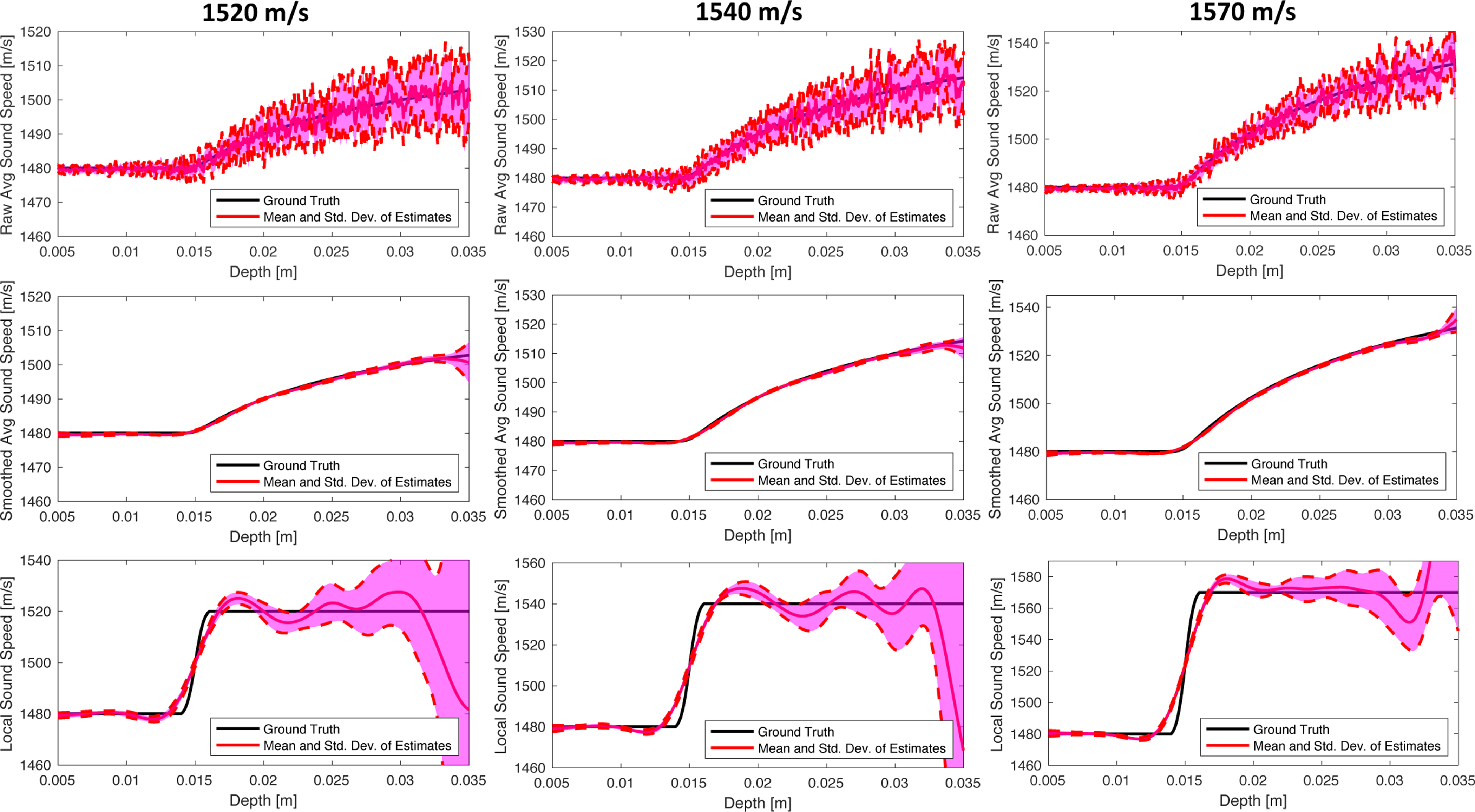
Estimation of the Average and Local Speeds of Sound in Three Two-Layer Media at 4 MHz Transmit Frequency. The sound speed is 1480 m/s over the first 15 mm in the medium and either 1520, 1540, or 1570 m/s in the rest of the medium. The raw average, smoothed average, and local sound speeds were estimated over 12 independent speckle realizations for each of the three two-layer media. The mean and standard deviation across speckle realizations is shown for each sound speed estimate as a function of depth. The standard deviation in the raw average and local sound speed estimates increase as a function of depth or, equivalently, f-number.

Fig. 8.

Estimation of the Average and Local Speeds of Sound in Three Two-Layer Media at 8 MHz. The same media as in Figure 7 are simulated at 8 MHz. The same sound speed estimates and statistics used in Figure 7 are calculated and shown here. The standard deviation in all sound speed estimates are smaller at 8 MHz than at 4 MHz (Figure 7).

TABLE III.

MEAN AND STANDARD DEVIATION OF LOCAL SOUND SPEED ESTIMATES IN TWO-LAYER MEDIA FROM 18 TO 25 MM DEPTH.

	1520 m/s in	1540 m/s in	1570 m/s in
	2nd Layer	2nd Layer	2nd Layer
4 MHz Transmit	1520.8±3.9	1541.6±3.7	1572.4±5.8
Frequency	m/s	m/s	m/s
8 MHz Transmit	1520.3±1.9	1541.0±2.4	1572.3±3.0
Frequency	m/s	m/s	m/s

Figure 9 demonstrates the sound speed estimation process in a phantom experiment in which a 5 mm thick porcine slab was placed on top of an ATS phantom (1460 m/s). Although the average sound speed is far from the sound speed in the phantom due to the porcine slab, the local sound speed estimates are close (within ±10 m/s) to the true sound speed in the ATS phantom from 10 to 30 mm depth. The strong coherent reverberation at roughly 6 mm depth causes a dip in the raw average sound speed measurement. At this location, the regularization smoothing decreases the slope of the smoothed average sound speed so that local sound speed estimates are erroneous around 6 mm depth. Sound speed values are not provided beyond 30mm because the standard deviation of the estimates becomes larger near at deepest imaging depth (35mm) where the fewest average sound speed measurements contribute to the local sound speed estimate. Figure 10 shows this sound speed estimation process repeated with four different imaging phantoms and six different imaging views per phantom. In these cases, the porcine layer on top of the phantoms was around 14–20 mm thick. For the ATS phantom and phantoms 1–3, the ground truth speed of sound inside the phantoms were 1460.0, 1489.7, 1516.2, and 1539.7 m/s, respectively. The mean and standard deviations in local sound speed estimates are plotted as a function of depth.

Fig. 9.

Sound Speed Estimation of the Average and Local Speeds of Sound in a Two-Layer Phantom Experiment. Although the average sound speed is far from the true sound speed in the phantom (1460 m/s) due to the high speed of sound in the porcine sample above the phantom (1570 m/s), the estimated local speed of sound in the phantom stays within ±10 m/s of the ground truth value from 10 to 30 mm depth.

Fig. 10.

Local Sound Speed Estimation in Four Different Phantoms. Mean and standard deviation in the the local sound speed estimates were compiled across 6 different imaging views. Bold lines indicate mean values and the dotted lines indicate the ± standard deviations in the measurement. For each phantom, the ground-truth speed of sound in the phantoms is shown from the starting depth of the phantom onwards. The ground truth sound speed in the phantoms were 1460.0±5.0, 1489.7±1.2, 1516.2±0.9, and 1539.7±0.7 in the ATS phantom and manufactured phantoms 1–3, respectively Local estimates tend to the follow the ground-truth sound speed value inside the phantom as the speed of sound inside the phantom is progressively increased.

D. Sound Speed Estimation in Rat Livers

Figure 11 shows the sound speed estimation process in the livers of two different rats. The single value reported for the effective average and local speeds of sound of each rat liver is an average of the estimates from 5 to 15 mm depth in the medium, as indicated by the green dashed lines shown. Below the green dashed lines the B-mode images show spinal bone and other structures that do not fit the layered medium assumption, and so sound speed estimation was not considered accurate in this region. The local sound speed estimate in the liver of the rat with a steatosis grade of 1 was 1562.8 m/s and its measured sound speed after excision was 1557 m/s. For the rat with a steatosis grade of 3, the local sound speed in the liver was estimated to be 1522.4 m/s, while the speed of sound measured in the excised liver was 1511 m/s. Figure 12 plots the average and local sound speed estimates against the ex-vivo sound speed measurement for each rat liver. The local sound speed estimates generally agree more strongly with ex-vivo sound speed measurement than the average sound speed. The regression line for local sound speed estimates is closer the line of equality (black dashed line) between imaging-based sound speed estimates and the ex-vivo measurements.

Fig. 11.

Example of Liver Imaging in Rats with Average and Local Sound Speed Estimates. (Top) The first rat shown is a female obese Zucker rat with a steatosis grade of 1. The local sound speed in the liver was measured to be 1562.8 m/s. The sound speed measured in the excised liver sample was 1557 m/s. (Bottom) The second rat is a female obese Zucker rat with a steatosis grade of 3. The local sound speed in the liver was measured to be 1522.4 m/s. The sound speed measured in the excised liver sample was 1511 m/s.

Fig. 12.

Average and Local Sound Speeds Estimates in Intact Abdominal Rat Livers vs Ex-Vivo Sound Speed Measurement in Excised Rat Livers. The black dashed line serves to indicate the condition of equality between the ex-vivo sound speed measurement and our imaging-based sound speed estimates. Local sound speed estimates (red) align better with the dashed-line than the average sound speed estimates (blue). The error bars signify the standard deviation in the sound speed estimate over the 5–15 mm depth range shown in Figure 11. The solid blue and red lines are regression lines over the average and local sound speed estimates, respectively.

V. DISCUSSION

The methodology in [23] used multi-lag least-squares cross-correlation [36] to compute residual delays after applying focusing delays to the multistatic channel data and summing across transmit elements. These residual delays were then added to the geometric delays used in focusing to compute a total delay curve for the scattering region. This delay curve was then squared prior to fitting to the parabolic model given by Anderson and Trahey [37] to obtain the average speed of sound. However, the sound speed estimation technique introduced by Anderson and Trahey [37] was initially proposed for determining this delay curve from receive-channel data following a single fixed-focus transmit beam, without any dynamic focusing applied to transmit or receive. In [23], dynamic focusing is applied to both transmit and receive prior to summing across transmit elements and estimating residual aberration delays by cross-correlating the receive channel data. In the presence of sound speed error, there is a broadening of the point spread function, which induces additional error in the time-delay between receive elements and alters the curvature of the residual aberration delays. This altered curvature in the residual aberration delays induces an error in the parabolic fit of the Anderson-Trahey method [37] and causes the estimation biases seen in Figures 3 and 4.

An alternative approach to [23] would be to synthesize receive-channel data for a fixed-focus transmit beam from the multistatic data, apply the methodology of Anderson and Trahey [37] to the non-time-delayed receive channel data as originally described, and estimate both the average sound speed and location of scattering from the parabolic fit. However, to estimate the local speed of sound in the medium, the average sound speed estimates may have to be placed on a potentially irregular grid of points axially in depth according to the estimated location of scattering.

Due to the difficulties of accurately estimating the effective average speed of sound without bias, the computational complexities of a cross-correlation based approach and the difficulties of gridding irregularly-sampled sound speed estimates, we applied a computationally-efficient estimation of the speed of sound that avoids this bias and estimates the speed of sound over a regularly-sampled grid in depth by using coherence maximization [14], [24], [25]. Figures 3 and 4 demonstrate that the coherence-based approach avoids these biases, and leads to more accurate estimates of the effective average and local speeds of sound. Figures 5 and 8 further validate this sound speed estimation approach in several homogeneous and two-layer media.

In Figure 6, it was shown that the CF curves were sharper around the true speed of sound for higher frequencies and lower f-numbers. As the speed of sound used to focus the channel data deviates from the true speed of sound in the medium, more phase variation is introduced across the receive aperture after focusing. As this phase variation increases, destructive interference across the aperture decreases the CF. Because phase is a product of frequency and delay, the amount of phase variation across the receive aperture increases as the frequency increases. This increase in phase variation with frequency decreases the CF, especially as the sound speed error increases, which leads to a narrowing of the CF curve around the true speed of sound in the medium. F-number affects the phase variation across the aperture by a different mechanism. As f-number increases, the geometric delay profile becomes flatter. Thus, when focusing at larger f-numbers, there is less phase variation across the aperture from a gross velocity error, which causes the CF curve to broaden around the true speed of sound in the medium.

For increasing reverberation strength, the amplitude of the CF curve decreases, but the sharpness is unchanged (Figure 6(d)). The sharpness is unchanged because the noise in reverberation is uncorrelated across the aperture, and thereby only decreases the CF curve’s amplitude. However, in the case of zero-mean aberration (Figure 6(c)), the aberration acts as correlated noise in the phase across the aperture. For small correlation lengths, there is no change to the sharpness of the CF curve as aberration strength increases because the resulting phase error appears similar to reverberation noise. For large correlation lengths, the sharpness of the curves decreases because the noise is correlated and reduces the phase variation across the aperture as the speed of sound is changed.

The impact of sharper CF curves on local sound speed estimation in layered media is observed in Figures 7 and 8. First, the standard deviation of all sound speed estimates is smaller at 8 MHz than at 4 MHz. Second, the standard deviation in the raw effective average speed of sound increases with depth, or equivalently f-number, because the aperture width is fixed. Based on Figure 6, CF is expected to become broader around the true speed of sound as f-number increases and frequency decreases.

The CF curve generally appears to be a quasiconcave function with respect to the focusing speed of sound. This correspondence between the broadness of the CF curve and the standard deviation of sound speed estimates in layered media is similar to the idea behind the Cramer-Rao lower bound´ (CRLB) for the variance of an unbiased estimator. Because CF maximization empirically appears to be an unbiased estimator of the speed of sound, the CRLB may be used to derive an expression for the lower bound on the standard deviation of the sound speed estimator; however, deriving an actual CRLB for this problem would require constructing a likelihood function parameterized by sound speed error for signals observed across the aperture based on the van-Cittert Zernike (VCZ) theorem [24]. Instead, if the CF curve is treated as a likelihood function, sound speed estimation exhibits the same behavior as the CRLB in that the standard deviation of sound speed estimates corresponds to the broadness of the CF curve. Future work on deriving an explicit Cramér-Rao bound for sound speed´ estimation could be used to further formalize the impact of various imaging conditions (e.g. f-number, frequency, phase aberration, or reverberation clutter) on the achievable accuracy of sound speed estimation.

Phantom and in-vivo experiments (Figures 9, 10, 11, and 12) further demonstrate the applicability of our sound speed estimator to channel data captured from an ultrasound scanner. In each case, the effective average sound speed is biased away from the true speed of sound in the phantom or the liver because of the high speed of sound (1570–1580 m/s) in the muscle tissue above it. However, the local sound speed estimates show significant agreement with the true sound speed in each case. A potential limitation of the in-vivo study was the euthania of the rats prior to imaging. However, a patient breath-hold may still enable the generalization of this work to a clinical setting given the relatively short data acquisition time. Applications of this technique on clinical scanners could be fat quantification based on the estimated speed of sound in the liver [15], [16], and phase aberration correction in tissues that resemble layered media.

VI. CONCLUSIONS

We demonstrated that a coherence-based approach to sound speed estimation can avoid the biases seen in our previous cross-correlation-based approach. Simulations show that our new coherence-based approach can be used to accurately estimate the average speed of sound, and subsequently, the local speed of sound in layered media. We also examined how imaging conditions such as f-number, frequency, phase aberration, and reverberation clutter affect our coherence-based approach. When applied to liver imaging in rats through the abdominal wall, the estimated local speed of sound showed significant agreement with direct ex-vivo sound speed measurements made on excised liver samples. In order to make our efforts more accessible to the broader research community, we have provided sample code and multistatic channel data for each of the three two-layer media at github.com/rehmanali1994/DixInversion4MedicalUltrasound (DOI: 10.5281/zenodo.4606777).

Biography

Rehman Ali received the B.S. degree in biomedical engineering from Georgia Institute of Technology (Atlanta, GA, USA) in 2016. He is currently an ND-SEG fellow, completing an M.S. in Computational & Mathematical Engineering and pursuing a Ph.D. in Electrical Engineering at Stanford. His research interests include signal processing, inverse problems, computational modeling of acoustics, and real-time beamforming algorithms. His current research is developing accurate and spatially resolved speed-of-sound imaging in tissue based on phase aberration correction and spatial coherence.

Huaijun Wang Dr. Wang’s interests are focused on exploring the diagnostic and therapeutic applications of ultrasound imaging. His research projects include treatment monitoring of inflammatory bowel disease in rodent and swine models with dual P- and E-selectin targeted ultrasound molecular imaging, therapeutic evaluation in tumors with 3-dimensional perfusion imaging and VEGF targeted ultrasound molecular imaging, early diagnosis of pancreatic cancer with Thy1-targeted ultrasound molecular imaging, and ultrasound-guided microbubble-mediated delivery of multiple microRNAs to improve chemotherapy in cancer.

Uday K. Sukumar received his B. Tech in Biotechnology followed by M.Tech and Ph.D in Nanotechnology from IIT-Roorkee in 2010, 2012 and 2016, respectively. After a brief stint at Nanotech start up (E-Spin Nanotech), he joined Dr. Paulmurugan’s lab at Department of Radiology, School of Medicine, Stanford University to pursue post-doctoral studies in the interdisciplinary field of nanobiotechnology. His research interest lies in exploring nano-enabled approaches for targeted therapeutic and diagnostic pre-clinical interventions. He specializes in synthesis, characterization and bio-evaluation of diverse nano formulations for ultrasound assisted targeted delivery of diagnostic nanomaterials as well as microRNA/suicide genes to orthotopic tumor models.

Jose G. Vilches-Moure, DVM, PhD, Assistant Professor, received his DVM degree from Purdue University in Indiana in 2007. He completed his residency training in Anatomic Pathology (with emphasis in pathology of laboratory animal species) and his PhD in Comparative Pathology at the University of California-Davis. He joined Stanford in 2015, and is the Director of the Animal Histology Services (AHS). Dr. Vilches-Moure is a diplomate of the American College of Veterinary Pathologists, and his collaborative research interests include cardiac development and pathology, developmental pathology, and refinement of animal models in which to study early cancer detection techniques. His teaching interests include comparative anatomy/histology, general pathology, comparative pathology, and pathology of laboratory animal species.

Ramasamy Paulmurugan received his master’s degree in biomedical genetics from the University of Madras, Chennai, India in 1991. In 1997, he earned his Ph.D. in Molecular Virology from the National Environmental Engineering Research Institute (NEERI), University of Madras, Chennai, India. After serving as a scientist for four years in Rajiv Gandhi Center for Biotechnology, Trivandrum, India, he joined University of California at Los Angeles (UCLA) as a visiting scientist in 2001. In 2003, he joined Stanford University as a senior research scientist to work under the Molecular Imaging Program at Stanford University (MIPS). Since 2009, he is an academic faculty in the Department of Radiology at Stanford University. Currently, his lab is working on developing in vivo molecular imaging assays to noninvasively monitor different epigenetic processes, and cancer early detection. His lab is also working on developing novel molecularly targeted therapies (microRNA and gene therapy) for various cancers, such as breast, hepatocellular carcinoma, and glioma.

Arsenii V. Telichko (Member, IEEE) Arsenii V. Telichko (Member, IEEE) received the B.S., M.S., and Ph.D. degrees from the Moscow Institute of Physics and Technology, Moscow, Russia, in 2011, 2013, and 2015, respectively. He joined Dr. Dahl?s lab at the Department of Radiology, School of Medicine, Stanford University, Stanford, CA, USA, as a Postdoctoral Fellow in 2016. In 2020, he was appointed as a Research Engineer at the Department of Radiology, School of Medicine, Stanford University. His research interests include intravascular imaging and transducer fabrication, elastography imaging, localized drug delivery with ultrasound, and cavitation detection. Recently, he has transitioned to industry and joined a local biotech start-up.

Jeremy J. Dahl (M’11) received the B.S. degree in electrical engineering from the University of Cincinnati (Cincinnati, OH, USA) in 1999, and the Ph.D. degree in biomedical engineering from Duke University (Durham, NC, USA) in 2004. He is currently an Associate Professor with the Department of Radiology at Stanford University, Stanford, CA, USA. His current research interests include beamforming, coherence and noise in ultrasonic imaging, speed of sound estimation, and ultrasound radiation force imaging technology.

REFERENCES

- [1].Pinton GF, Trahey GE, and Dahl JJ, “Sources of image degradation in fundamental and harmonic ultrasound imaging using nonlinear, full-wave simulations,” IEEE transactions on ultrasonics, ferroelectrics, and frequency control, vol. 58, no. 4, 2011. [DOI] [PMC free article] [PubMed] [Google Scholar]
- [2].Hayashi N, Tamaki N, Senda M, Yamamoto K, Yonekura Y, Torizuka K, Ogawa T, Katakura K, Umemura C, and Kodama M, “A new method of measuring in vivo sound speed in the reflection mode,” Journal of clinical ultrasound, vol. 16, no. 2, pp. 87–93, 1988. [DOI] [PubMed] [Google Scholar]
- [3].Jaeger M, Held G, Peeters S, Preisser S, Grünig M, and Frenz M, “Computed ultrasound tomography in echo mode for imaging speed of sound using pulse-echo sonography: proof of principle,” Ultrasound in medicine & biology, vol. 41, no. 1, pp. 235–250, 2015. [DOI] [PubMed] [Google Scholar]
- [4].Stähli P, Kuriakose M, Frenz M, and Jaeger M, “Improved forward¨ model for quantitative pulse-echo speed-of-sound imaging,” Ultrasonics, p. 106168, 2020. [DOI] [PubMed] [Google Scholar]
- [5].Sanabria SJ, Ozkan E, Rominger M, and Goksel O, “Spatial domain reconstruction for imaging speed-of-sound with pulse-echo ultrasound: simulation and in vivo study,” Physics in Medicine & Biology, vol. 63, no. 21, p. 215015, 2018. [DOI] [PubMed] [Google Scholar]
- [6].Rau R, Schweizer D, Vishnevskiy V, and Goksel O, “Speed-of-sound imaging using diverging waves,” arXiv preprint arXiv:1910.05935, 2019. [DOI] [PMC free article] [PubMed] [Google Scholar]
- [7].Stähli P, Frenz M, and Jaeger M, “Bayesian approach for a robust¨ speed-of-sound reconstruction using pulse-echo ultrasound,” IEEE transactions on medical imaging, vol. 40, no. 2, pp. 457–467, 2020. [DOI] [PubMed] [Google Scholar]
- [8].Greenleaf JF and Bahn RC, “Clinical imaging with transmissive ultrasonic computerized tomography,” IEEE Transactions on Biomedical Engineering, no. 2, pp. 177–185, 1981. [DOI] [PubMed] [Google Scholar]
- [9].Pérez-Liva M, Herraiz J, Udías J, Miller E, Cox B, and Treeby B, “Time domain reconstruction of sound speed and attenuation in ultrasound computed tomography using full wave inversion,” The Journal of the Acoustical Society of America, vol. 141, no. 3, pp. 1595–1604, 2017. [DOI] [PubMed] [Google Scholar]
- [10].André M, Wiskin J, and Borup D, “Clinical results with ultrasound´ computed tomography of the breast,” in Quantitative Ultrasound in Soft Tissues. Springer, 2013, pp. 395–432. [Google Scholar]
- [11].Podkowa A, Hidayetoglu M, Yang C, Oelze M, and Chew WC, “Reconstruction of sound speed distributions from pulse-echo data,” The Journal of the Acoustical Society of America, vol. 140, no. 4, pp. 3373–3373, 2016. [Google Scholar]
- [12].Podkowa A and Oelze M, “Echo-mode aberration tomography: Sound speed imaging with a single linear array,” The Journal of the Acoustical Society of America, vol. 145, no. 3, pp. 1859–1859, 2019. [Google Scholar]
- [13].Podkowa AS and Oelze ML, “The convolutional interpretation of registration-based plane wave steered pulse-echo local sound speed estimators,” Physics in Medicine & Biology, vol. 65, no. 2, p. 025003, 2020. [DOI] [PubMed] [Google Scholar]
- [14].Ali R and Dahl JJ, “Distributed phase aberration correction techniques based on local sound speed estimates,” in 2018. IEEE International Ultrasonics Symposium (IUS). IEEE, 2018, pp. 1–4. [DOI] [PMC free article] [PubMed] [Google Scholar]
- [15].Imbault M, Faccinetto A, Osmanski B-F, Tissier A, Deffieux T, Gennisson J-L, Vilgrain V, and Tanter M, “Robust sound speed estimation for ultrasound-based hepatic steatosis assessment,” Physics in Medicine & Biology, vol. 62, no. 9, p. 3582, 2017. [DOI] [PubMed] [Google Scholar]
- [16].Imbault M, Burgio MD, Faccinetto A, Ronot M, Bendjador H, Deffieux T, Triquet EO, Rautou P-E, Castera L, Gennisson J-L et al. , “Ultrasonic fat fraction quantification using in vivo adaptive sound speed estimation,” Physics in Medicine & Biology, vol. 63, no. 21, p. 215013, 2018. [DOI] [PubMed] [Google Scholar]
- [17].Lambert W, Cobus LA, Couade M, Fink M, and Aubry A, “Reflection matrix approach for quantitative imaging of scattering media,” Physical Review X, vol. 10, no. 2, p. 021048, 2020. [Google Scholar]
- [18].Jaeger M, Robinson E, Akarc HG¸ay, and M. Frenz, “Full correction for spatially distributed speed-of-sound in echo ultrasound based on measuring aberration delays via transmit beam steering,” Physics in medicine & biology, vol. 60, no. 11, p. 4497, 2015. [DOI] [PubMed] [Google Scholar]
- [19].Sehgal C, Brown G, Bahn R, and Greenleaf JF, “Measurement and use of acoustic nonlinearity and sound speed to estimate composition of excised livers,” Ultrasound in medicine & biology, vol. 12, no. 11, pp. 865–874, 1986. [DOI] [PubMed] [Google Scholar]
- [20].Lin T, Ophir J, and Potter G, “Correlations of sound speed with tissue constituents in normal and diffuse liver disease,” Ultrasonic imaging, vol. 9, no. 1, pp. 29–40, 1987. [DOI] [PubMed] [Google Scholar]
- [21].Tervola K, Gummer M, Erdman J Jr, and OBrien W Jr, “Ultrasonic attenuation and velocity properties in rat liver as a function of fat concentration: A study at 100 mhz using a scanning laser acoustic microscope,” The Journal of the Acoustical Society of America, vol. 77, no. 1, pp. 307–313, 1985. [DOI] [PubMed] [Google Scholar]
- [22].Burgio MD, Imbault M, Ronot M, Faccinetto A, Van Beers BE, Rautou P-E, Castera L, Gennisson J-L, Tanter M, and Vilgrain V, “Ultrasonic adaptive sound speed estimation for the diagnosis and quantification of hepatic steatosis: a pilot study,” Ultraschall in der Medizin-European Journal of Ultrasound, 2018. [DOI] [PubMed] [Google Scholar]
- [23].Jakovljevic M, Hsieh S, Ali R, Chau Loo Kung G, Hyun D, and Dahl JJ, “Local speed of sound estimation in tissue using pulse-echo ultrasound: Model-based approach,” The Journal of the Acoustical Society of America, vol. 144, no. 1, pp. 254–266, 2018. [DOI] [PMC free article] [PubMed] [Google Scholar]
- [24].Mallart R and Fink M, “Adaptive focusing in scattering media through sound-speed inhomogeneities: The van cittert zernike approach and focusing criterion,” The Journal of the Acoustical Society of America, vol. 96, no. 6, pp. 3721–3732, 1994. [Google Scholar]
- [25].Yoon C, Lee Y, Chang JH, Song T.-k., and Yoo Y, “In vitro estimation of mean sound speed based on minimum average phase variance in medical ultrasound imaging,” Ultrasonics, vol. 51, no. 7, pp. 795–802, 2011. [DOI] [PubMed] [Google Scholar]
- [26].Hyun D, Crowley ALC, and Dahl JJ, “Efficient strategies for estimating the spatial coherence of backscatter,” IEEE transactions on ultrasonics, ferroelectrics, and frequency control, vol. 64, no. 3, pp. 500–513, 2017. [DOI] [PMC free article] [PubMed] [Google Scholar]
- [27].Dix CH, “Seismic velocities from surface measurements,” Geophysics, vol. 20, no. 1, pp. 68–86, 1955. [Google Scholar]
- [28].Neidell NS and Taner MT, “Semblance and other coherency measures for multichannel data,” Geophysics, vol. 36, no. 3, pp. 482–497, 1971. [Google Scholar]
- [29].Jensen JA, “Simulation of advanced ultrasound systems using field ii,” in 4th IEEE International Symposium on Biomedical Imaging: From Nano to Macro. IEEE, 2004, pp. 636–639. [Google Scholar]
- [30].Dahl JJ and Sheth NM, “Reverberation clutter from subcutaneous tissue layers: Simulation and in vivo demonstrations,” Ultrasound Med Biol, vol. 40, no. 4, pp. 714–726, 2014. [DOI] [PMC free article] [PubMed] [Google Scholar]
- [31].Lediju M, Trahey GE, Byram BC, and Dahl JJ, “Short-lag spatial coherence of backscattered echoes: Imaging characteristics,” IEEE Transactions on Ultrasonics, Ferroelectrics, and Frequency Control, vol. 58, no. 7, pp. 1377–1388, 2011. [DOI] [PMC free article] [PubMed] [Google Scholar]
- [32].Pinton GF, Trahey GE, and Dahl JJ, “Spatial coherence in human tissue: Implications for imaging and measurement,” IEEE Transactions on Ultrasonics, Ferroelectrics, and Frequency Control, vol. 61, no. 12, pp. 1976–1987, 2014. [DOI] [PMC free article] [PubMed] [Google Scholar]
- [33].Treeby BE and Cox BT, “k-wave: Matlab toolbox for the simulation and reconstruction of photoacoustic wave fields,” Journal of biomedical optics, vol. 15, no. 2, p. 021314, 2010. [DOI] [PubMed] [Google Scholar]
- [34].Burlew MM, Madsen EL, Zagzebski JA, Banjavic RA, and Sum SW, “A new ultrasound tissue-equivalent material.” Radiology, vol. 134, no. 2, pp. 517–520, 1980. [DOI] [PubMed] [Google Scholar]
- [35].Kuo I, Hete B, and Shung K, “A novel method for the measurement of acoustic speed,” The Journal of the Acoustical Society of America, vol. 88, no. 4, pp. 1679–1682, 1990. [DOI] [PubMed] [Google Scholar]
- [36].Ivancevich NM, Dahl JJ, and Smith SW, “Comparison of 3-d multi-lag cross-correlation and speckle brightness aberration correction algorithms on static and moving targets,” IEEE transactions on ultrasonics, ferroelectrics, and frequency control, vol. 56, no. 10, pp. 2157–2166, 2009. [DOI] [PMC free article] [PubMed] [Google Scholar]
- [37].Anderson ME and Trahey GE, “The direct estimation of sound speed using pulse–echo ultrasound,” The Journal of the Acoustical Society of America, vol. 104, no. 5, pp. 3099–3106, 1998. [DOI] [PubMed] [Google Scholar]