

Abstract
The presence of two longitudinal waves in porous media is predicted by Biot’s theory and has been confirmed experimentally in cancellous bone. When cancellous bone samples are interrogated in through-transmission, these two waves can overlap in time. Previously, the Modified Least-Squares Prony’s (MLSP) method was validated for estimation of amplitudes, attenuation coefficients, and phase velocities of fast and slow waves, but tended to overestimate phase velocities by up to about 5%. In the present paper, a pre-processing chirp filter to mitigate the phase velocity bias is derived. The MLSP / chirp filter (MLSPCF) method was tested for decomposition of a 500 kHz-center-frequency signal containing two overlapping components: one passing through a low-density-polyethylene plate (fast wave) and another passing through a cancellous-bone-mimicking phantom material (slow wave). The chirp filter reduced phase velocity bias from 100 m/s (5.1%) to 69 m/s (3.5%) (fast wave) and from 29 m/s (1.9%) to 10 m/s (0.7%) (slow wave). Similar improvements were found for 1) measurements in polycarbonate (fast wave) and a cancellous-bone-mimicking phantom (slow wave), and 2) a simulation based on parameters mimicking bovine cancellous bone. The MLSPCF method did not offer consistent improvement in estimates of attenuation coefficient or amplitude.
Keywords: Prony’s method, cancellous bone, attenuation, phase velocity
I. INTRODUCTION
Quantitative ultrasound is emerging as an increasingly important modality for characterization of bone (Laugier, 2008). Recent technological developments include increased portability (Kaufman et al., 2007), expansion to new sites such as the radius (Le Floch et al., 2008), femur (Barkmann et al., 2008) and tibia (Sarvazyan et al., 2009), and a dual-frequency pulse-echo method for removing effects of soft tissues (Riekkinen et al., 2006, 2008).
Cancellous bone consists of a porous mineralized trabecular network with a fluid filler (marrow in vivo or water in vitro). Through-transmission measurements of cancellous bone samples immersed in water sometimes show the existence of two compressional waves propagating in the bone (Hosokawa and Otani 1997, 1998; Hughes et al. 1999; Kaczmarek et al. 2002; Cardoso et al. 2003; Mizuno et al., 2008). The existence of two compressional waves in porous media is predicted by Biot theory (Biot 1956a, 1956b, 1956c, 1962, 1963), which has been applied to bone by many investigators (McKelvie and Palmer 1991; Williams 1992; Hosokawa and Otani 1997, 1998; Haire and Langton 1999; Pakula and Kubik, 2002; Hughes et al. 2003; Lee et al. 2003; Mohamed et al. 2003; Cardoso et al. 2003; Fellah et al. 2004; Hosokawa, 2005; Wear et al. 2005; Lee and Yoon 2006; Hughes et al. 2007; Pakula et al. 2008; Fellah et al. 2008; Sebaa et al. 2008; Cardoso et al., 2008; Cowin and Cardoso, 2010). A new clinical device evaluates separately propagation speed and amplitude of fast and slow waves at the distal radius (Breban et al., 2010). Within the Biot theory, two compressional waves correspond to the fluid and solid moving in-phase (fast wave) and out-of-phase (slow wave) with each other.
If fast and slow waves can be separated, their properties (amplitude, attenuation coefficient, and phase velocity), convey important information regarding material and structural properties of cancellous bone. Experiments on bone samples in vitro suggest that the fast and slow waves have different frequency-dependent attenuation coefficients (Hosokawa and Otani 1997; Kaczmarek et al. 2002; Cardoso et al. 2003). Fast wave velocity in bovine cancellous bone depends on structural anisotropy and is maximum when propagation is parallel to the trabecular orientation (Mizuno et al., 2008). Theoretical analysis suggests that the relative amplitudes of fast and slow waves are sensitive to bone volume fraction, sample thickness, tortuosity, and viscous characteristic length (Fellah et al. 2004). Three-dimensional finite-difference time-domain simulations suggest that fast wave velocity is much more sensitive to bone volume fraction than slow wave velocity (Haïat et al. 2008; Hosokawa 2008) and that fast and slow wave attenuation coefficients exhibit markedly different dependencies on bone volume fraction (Hosokawa, 2008).
Separate analysis of fast and slow waves is often difficult for cancellous bone samples in vitro because the two waves often overlap in time due to 1) insufficient contrast between fast and slow wave velocities and/or 2) insufficient sample thickness. The contrast between fast and slow velocities is lower when the ultrasound propagation direction is perpendicular (compared with parallel) to the predominant trabecular orientation (Hosokawa and Otani 1997, 1998). The degree of structural anisotropy influences the temporal separability of fast and slow waves (Haïat et al. 2008). A low correlation coefficient between transmission signal loss and frequency may be used to indicate the simultaneous presence of multiple waves such as fast and slow waves from Biot theory or waves traversing multiple paths through the bone (Haïat et al. 2008).
A Bayesian method was shown to be effective for separation of overlapping time-domain pulses for simulated signals mimicking measurements from cancellous bone (Marutyan et al. 2007). This method involves calculations using Markov chain Monte Carlo with simulated annealing. Although the Bayesian method is a valuable tool for investigation of the interaction between ultrasound and cancellous bone, it may not be practical for some researchers since the computer code is complicated, and the processing time can be lengthy (100 minutes on a Sun Enterprise 250 dual 400-MHz workstation) unless a cluster of processors is used (3 minutes using 32 processors on an SGI Altix 3000 with Itanium2 processors running at 900 MHz) (Marutyan et al. 2007).
Previously, the Modified Least-Squares Prony’s (MLSP) method was shown to be effective for estimation of amplitude, attenuation, and phase velocity of both fast and slow waves, but tended to consistently overestimate phase velocity by up to about 4.3% (fast wave) and 1.3% (slow wave) (Wear, 2010). The MLSP method models a signal as a sum of exponentially-damped sinusoids and recovers four parameters for each component (amplitude, decay rate, oscillation rate, and initial phase). It may be applied to the ratio of through-transmission spectra with and without cancellous bone in a water path when that spectral ratio function is a sum of exponentially-damped sinusoids (Wear, 2010). This form of the spectral ratio function was proposed by Marutyan et al. (2006).
In the present paper, a pre-processing chirp filter (applied prior to application of the MLSP method) to mitigate the MLSP bias is derived and tested. The decomposition of a mixed pulse into its two components becomes increasingly difficult as 1) signal-to-noise (SNR) decreases, 2) the fast wave velocity approaches the slow wave velocity, or 3) the ratio of the energy in the low-amplitude wave to the energy in the high-amplitude wave decreases. In the present paper, the first two effects are investigated with computer simulations (using parameters that correspond to bovine cancellous bone), and the third effect is investigated with an experiment.
II. THEORY
A. Two-wave model
The model used here is adapted from a previous model (Marutyan et al., 2006) for composite media such as cancellous bone that exhibit two waves propagating simultaneously through a linear-with-frequency attenuating medium. The model assumes two co-axial transducers in a through-transmission or “pitch/catch” orientation. If X(ω) is the spectrum of the signal passing through a water-only path and Y(ω) is the spectrum of the signal passing through a water-sample-water path, then,
| (1) |
where
| (2) |
| ω = 2πf | and f is the ultrasound frequency, |
| Aj | includes the effects of transmission through boundaries, |
| αj(ω) = | attenuation coefficient = βj
ω / 2π, |
| βj = | attenuation coefficient slope |
| vj(ω) = | phase velocity, |
| d = | sample thickness, |
| c = | speed of sound in water, |
and j stands for either fast or slow.
This expression includes an exponential factor, exp[-i ωd/c], to explicitly account for the fact that, in a substitution experiment, the attenuating sample replaces an equivalent length of water in the acoustic beam path. Marutyan et al. (2006) used Hj(ω) to describe the effect of sample itself (not necessarily the spectral ratio from a substitution experiment) and therefore omitted this exponential factor. The model neglects attenuation due to water and diffraction effects, which can be significant when the thickness and sound speed contrast between the reference and experimental media are sufficiently great (Kaufman et al., 1995) but are typically small for cancellous bone samples (Kaufman et al., 1995; Droin et al., 1998). The two-wave model can predict negative dispersion (Anderson, 2008), which has been reported in human cancellous bone (Nicholson et al., 1996; Stelitzki et al., 1996; Droin et al., 1998; Wear, 2000). In the event that the fast wave attenuation coefficient is a function of propagation distance, as has been reported in a numerical and experimental study of wave attenuation in cancellous bone (Nagatani, et al., 2008), the fast wave attenuation coefficient in Equations 1 and 2, αfast(ω), would represent a spatially-averaged effective fast wave attenuation coefficient.
In previous reports, functions that describe through-transmission substitution experiments that have forms similar to Equation 2 above have been referred to as “transfer functions” (Wear, 2009; Wear, 2010). This terminology could be misleading when 1) a transfer function is taken to refer to the ratio of output to input spectra, and 2) the output time-domain signal is required to be zero until the input time-domain signal becomes nonzero. For example, if the speed of sound is faster in the sample than in water, then y(t), the inverse Fourier Transform of Y(ω), may become nonzero before x(t), the inverse Fourier Transform of X(ω). Therefore, a function that describes a through-transmission substitution experiment and has a form similar to Equation 2 might preferably be called a “through-transmission spectral ratio” or “transmission coefficient.”
B. Prony’s Method and Variants
Prony’s method and its variants model a digitized complex signal, x[1], x[2], x[3], …, x[N], as the sum of p exponentially-damped sinusoids as follows (Marple, 1987):
| (3) |
where Aj is an amplitude, sj is a damping rate, qj is an oscillation rate, and θj is an initial phase of the jth complex exponential. Δω is the sample interval. In Equation 3, Marple’s notation has been modified in order to reduce confusion that may arise from the fact that while the most common application of Prony’s method and its variants is modeling a time domain signal, the present application is modeling a frequency domain signal.
By comparing Equation 3 with Equations 1 and 2, the following correspondences can be made:
p = 2,
ω = (n-1) Δω,
sj = - βj d / 2π,
, and
θj = 0 (with no loss in generality if Aj are allowed to be complex).
In Equation 3, the frequency-dependence of phase velocities, vj(ω), has been ignored so that vj(ω) ≈ vj(ω0) where ω0 = 2πf0 and f0 is a reference frequency such as the transducer center frequency. The frequency dependence of the phase velocities (i.e., dispersion) will be considered in the next section.
Prony’s method and its variants have been described in great detail elsewhere (Marple, 1987). Prony’s original method was designed for cases when the number of data points equals the number of parameters to be estimated. In this case, an exact fit of the model to the data may be performed. When the number of data points exceeds the number of parameters to be estimated, the MLSP method may be used to generate an approximate fit of the model to the data. Prony’s method and its variants consist of three steps. First, the data are fit to a linear prediction model. Then, estimates for damping rates and oscillation rates are obtained from the roots of a polynomial formed from the linear prediction coefficients obtained in step 1. Finally, estimates for amplitudes and initial phases are obtained from the solution of a set of linear equations. For more detail, see (Marple 1987).
C. Dispersion and the Chirp Filter
Equation (3) is directly applicable in the absence of dispersion. However, the nearly local form of the Kramers-Kronig relations for media with linear-with-frequency attenuation predicts the following dispersion relation (O’Donnell et al., 1981, Waters et al., 2000, Waters et al., 2005; Anderson et al.,, 2008)
| (4) |
This expression is valid for small dispersion. (Dispersion increases with attenuation slope, but Figure 1 shows that even for typical parameters for the highly-attenuated fast wave, phase velocity changes by only a few percent within a typical transducer bandwidth centered at 1 MHz.) Models based on fast and slow waves obeying this dispersion relation have been shown to be consistent with measurements of frequency-dependent phase velocity in cancellous bone (Marutyan, et al., 2006; Anderson et al., 2008).
Figure 1.

Phase velocity of the form of Equation (4) with first and second order Taylor series approximations for a case where v(ω0) = 2100 m/s and β = 20 dB/cmMHz.
In order to investigate the effects of dispersion, it is useful to approximate vj(ω) as a Taylor expansion about the center frequency, ω0.
| (5) |
Let the coefficients in the expansion be denoted by A, B, and C.
| (6) |
where (from Equation 4) A = vj(ω0), B = vj(ω0)2 βj / (π2ω0), and C = - vj(ω0)2 βj / (2π2ω02). Figure 1 shows a phase velocity function of the form of Equation (4) with first and second order Taylor series approximations. For a range of frequencies near the center frequency (1 MHz), the second order Taylor series approximation agrees quite well with the logarithmically-varying phase velocity.
The velocity-dependent exponential factor in Equation 2, exp[iωd/vj(ω)], may be approximated over the experimental band of frequencies for a weakly-dispersive medium, i.e., (B/A)(ω-ω0) << 1 and (C/A)(ω-ω0)2 << 1. First, the reciprocal of the velocity may be approximated as follows.
| (7) |
Now
| (8) |
Therefore, the Hj(ω) for each wave takes the form,
| (9) |
The first, second, and fifth exponential factors in Equation 9 are compatible with the damped sinusoidal form assumed by Prony’s method and its variants. However, the third and fourth exponential factors cause the signal to deviate from a simple, damped sinusoidal form. The distortion is in the form of a chirp function. The effects of this chirp distortion can be mitigated by filtering (i.e., multiplying) Hj(ω) with an inverse chirp filter, D(ω; β) prior to applying Prony’s method.
| (10) |
where
| (11) |
D(ω; β) is an all-pass filter that does not depend on phase velocity but does depend on attenuation coefficient slope, β. Therefore, a value for β must be selected prior to computation of the filter function. Reasonably accurate preliminary estimates for βfast and βslow may be obtained by applying the MLSP method without chirp filtering (Wear, 2010). A conservative approach for the MLSPCF method would be to set the value of β in D(ω; β) to the minimum of and , which can be denoted as . D(ω; ) would approximately cancel the chirp distortion for the minimum-β wave (assuming that is a good estimate of the true βmin ) and at least mitigate the chirp distortion for the maximum-β wave. This approach will be referred to hereafter in this paper as the “conservative” chirp filter. An alternative approach, which will be referred to hereafter in this paper as the “dual” (i.e., two-channel) chirp filter, would be to apply the MSLPCF method in two separate steps: 1) filtering Htotal(ω) with D(ω; ) to estimate the properties of the minimum-β wave, and 2) filtering Htotal(ω) with D(ω; β2) to estimate the properties of the maximum-β wave. Candidate values for β2 include 1) (weighted average), and 2) (maximum-β). The conservative and dual approaches give identical results (by definition) for the minimum-β wave but give different results for the maximum-β wave.
III. METHODS
A. Simulation
A simulation was performed to investigate the dependencies of the MLSP and MLSPCF estimates of parameter values—Aj, βj, and vj(ω0)—on signal-to-noise ratio (SNR) and fast/slow velocity differential, using parameters reported for bovine cancellous bone. Simulated waveforms were generated using Equations 1, 2, and 4. The parameters of the waveforms were d = 1 cm, Afast = 0.75, Aslow = 0.25, βfast = 20 dB/cmMHz, βslow = 6.9 dB/cmMHz, vfast(ω0) ranging from 1600 to 2100 m/s, and vslow(ω0) = 1500 m/s (Hosokawa and Otani 1997; Waters and Hoffmeister 2005; Anderson et al. 2008) where ω0 = 2πf0 and f0 = 1 MHz. In order to ensure temporal overlap between fast and slow waves, 1) the slow wave velocity was taken to be near the upper limit of the range reported for bovine cancellous bone (Hosokawa and Otani, 1997; Kaczmarek et al., 2002; Cardoso et al., 2003), and 2) the sample thickness and fast wave phase velocities were restricted to relatively small values. (If fast and slow waves do not overlap, then the task of measuring separate fast and slow wave properties is trivial.) X(ω) was a Gaussian function, exp[−(f-f0)2 / 2σ2] with f0 = 1 MHz and σ = 0.2 MHz. Gaussian white noise was added to the RF waveforms to generate signals with SNR’s ranging from 20 to 50 dB. SNR was defined as the ratio of the maximum time-domain pulse amplitude of y(t), the inverse Fourier Transform of Y(ω), to the average time-domain amplitude of the Gaussian white noise. The MLSP and MLSPCF methods were applied to Y(ω) / X(ω), over the range from 0.5 to 1.5 MHz. Six hundred trials were generated for each value of SNR and fast wave velocity.
B. LDPE / Cancellous-Bone-Mimicking-Phantom Slab Experiment
The first experiment involved a test sample that consisted of an 11-mm-thick low-density polyethylene (LDPE) plate (fast wave) bonded to an 11-mm-thick slab of cancellous-bone-mimicking material (cut from Model 063 CIRS Inc., Norfolk, VA, USA) (slow wave). The cancellous-bone-mimicking material consisted of homogeneous proprietary urethane material that mimicked the frequency-dependent attenuation and sound speed, but not the micro-architecture, of cancellous bone. The 11-mm-thick composite was placed in the ultrasound beam so that half the beam passed through 11 mm of LDPE and half the beam passed through 11 mm of cancellous-bone-mimicking material. The use of two bonded plates/slabs to produce simultaneous fast and slow waves was first proposed by Anderson et al. (2009), who used acrylic and polycarbonate plates. Measurements were also performed with the beam passing through pure LDPE or pure bone-mimicking phantom material in order to obtain independent measurements of the wave parameters—Aj, βj, and vj(ω0)—for the two media to compare with the MLSP- and MLSPCF-derived values. In all experiments, interfaces were oriented perpendicular to the beam in order to minimize refraction artifact.
C. Polycarbonate / Cancellous-Bone-Mimicking Phantom Experiment
The second experiment was performed to investigate the dependences of the MLSP- and MLSPCF-method estimates of wave parameter values—βj and vj(ω0)—on the relative time-domain amplitudes of the fast and slow waves. It can be difficult to produce composite specimens in which the relative amplitudes of the fast and slow waves can be finely adjusted. Therefore, in the present study, a simplified but mathematically equivalent experiment was performed as follows. First, a through-transmission calibration measurement was performed through a water-only path. Second, a through-transmission measurement was performed through a 25-mm-thick polycarbonate plate (fast wave). Third, a through-transmission measurement was performed through a commercially-available 36-mm-thick cancellous bone phantom (slow wave) (Model 063 CIRS Inc., Norfolk, VA, USA). Fourth, the digitized radio-frequency (RF) signals from the two measurements were weighted and added in software in order to simulate a measurement that would be obtained from a composite medium. The thicknesses and sound speeds of the two materials resulted in significant overlap between the time-domain signals, as demonstrated previously (Wear, 2010). In order to investigate the performances of the MLSP and MLSPCF methods as functions of relative fast / slow signal relative time-domain peak amplitudes, nine different weight pairs were used to generate data with fast wave / slow wave signal relative time-domain peak amplitudes equal to 10% / 90%, 20% / 80%, … 90% / 10%.
D. Ultrasound Data Acquisition System
A pulser/receiver (5077PR, Panametrics, Waltham, MA, USA) and a pair of coaxially-aligned, 500 kHz, broadband, 0.75” (1.9 cm) diameter, 1.5” (3.8 cm) focal length transducers (Panametrics, V301, Waltham, MA, USA) were used to interrogate samples in a water tank. The propagation path between transducers was twice the focal length. Received RF signals were digitized (8 bit, 25 MHz) using an oscilloscope (LeCroy, 9310C, Chestnut Ridge, NY, USA) and stored on computer (via general purpose interface bus) for off-line analysis. Ten RF signals were averaged for each through-transmission measurement. Multiple measurements were performed, with repositioning between measurements, and the estimated parameters were averaged over all measurements. Ten measurements (based on 100 RF signals with 10 repositionings) were performed for the LDPE / bone-mimicking phantom slab experiment. Four measurements (based on 40 RF signals with 4 repositionings) were performed for both the polycarbonate plate and for the bone-mimicking phantom.
E. Data Analysis
For the LDPE / bone-mimicking phantom slab experiment, spectra for the two signals—i.e., 1: pure water signal, and 2: 50% LDPE (left half of the beam) / 50% bone-mimicking phantom signal (right half of the beam)—were computed using Fast Fourier Transforms (FFT’s). The ratio of these spectra yielded Htotal(ω).
For the simulation and the polycarbonate / bone-mimicking phantom experiment, spectra for each of the four signals (i.e., 1: pure water signal, 2: fast wave, 3: slow wave, and 4: time-domain sum of fast and slow waves) were computed using FFT’s. The ratio of the fast-wave spectrum to the water-only-path spectrum yielded Hfast(ω) (see Equation 1). The ratio of the slow-wave spectrum to the water-only path spectrum yielded Hslow(ω). The ratio of the weighted, summed signal (fast wave plus slow wave) spectrum to the water-only-path spectrum path yielded Htotal(ω).
Estimates of wave parameters—Aj, βj, and vj(ω0)—were obtained by applying the MLSP and MLSPCF methods directly to Htotal(ω). In order to assess the accuracies of the MLSP and MLSPCF methods, these estimates were compared to reference values for wave parameters. The reference wave parameter values were known a priori for the computer simulated data and were measured for the experimental data using the following conventional methods.
Attenuation coefficients for the polycarbonate plate, LDPE plate, cancellous-bone-mimicking phantom, and cancellous-bone-mimicking phantom slab were estimated using a log spectral difference technique (Kuc and Schwartz 1979).
| (13) |
where Sw(ω) is the power spectrum from a water-only path and Sj(ω) is the power spectrum from either the LDPE plate (first experiment), 11-mm-thick cancellous bone-mimicking phantom slab (first experiment), polycarbonate plate (second experiment) or 36-mm-thick cancellous bone-mimicking phantom (second experiment). Since the attenuation coefficients for all these materials were very nearly linear with frequency, they could be accurately characterized by the slope of a least-squares linear fit of attenuation coefficient (dB/cm) vs. frequency over the range from 200 to 800 kHz.
Frequency-dependent phase velocities for the polycarbonate plate, LDPE plate, cancellous-bone-mimicking phantom, and cancellous-bone-mimicking phantom slab were computed using
| (14) |
where Δϕ(ω) is the difference in unwrapped phases (see next paragraph) of the received signals with and without the sample in the water path, d is the sample thickness, c is the temperature-dependent speed of sound in distilled water (Pierce, 1981). The equation for phase velocity (Equation 14) is often reported with a plus sign instead of a minus sign in the denominator. The ambiguity arises from ambiguity in Δϕ(ω), which may be computed as ϕ(ω) − ϕw(ω) or ϕw(ω) − ϕ(ω). Temperature, measured with a digital thermometer, was 18.6° for these measurements, which meant that c was about 1477 m/s.
The unwrapped phase difference, Δϕ(ω), was computed as follows. FFT’s of the digitized received signals were taken. The phase of the signal at each frequency was taken to be the inverse tangent of the ratio of the imaginary to real parts of the FFT at that frequency. Since the inverse tangent function yields principal values between −π and π, the phase had to be unwrapped by adding an integer multiple of 2π to all frequencies above each frequency where a discontinuity appeared.
The routine mprony.m from StatBox 4.2 (StatSci.org, 2010) was used to perform modified Prony method computations in Matlab (Mathworks, Natick, MA). (Note: The adjective “modified” has been used in conjunction with Prony’s method in multiple ways. Here the term is used in the sense of Osborne and Smyth (1995).) Model orders for values of p = 2, 3, 4, 5, and 6 were applied to each waveform. Previous investigators have shown that in the presence of noise, biases in parameter estimates may be reduced by selecting model orders higher than the number of exponentials actually in the signal (Van Blaricum and Mittra, 1975; Kumaresan and Tufts, 1982; Marple, 1987). This is reasonable because the model should be able to accommodate not only the energy in the signal but also the energy in the noise as well. For p > 2, the two waves with maximum total energy were designated as the two signal waves. The wave with the faster velocity was designated as the fast wave, Hfast(ω), and the wave with the slower velocity was designated as the slow wave, Hslow(ω). The model estimate was the sum of the two highest energy waves, Hfast(ω) + Hslow(ω). The order (p) that produced the minimum final prediction error (FPE) between the model and the simulated H(ω) was designated as the optimum order, where
| (15) |
ρp is the prediction error power, and N is the number of samples in the estimate for H(ω) (Marple, 1987). The means and standard deviations for the wave parameter estimates—Aj, βj, and vj(ω0)—were computed both with and without chirp filtering
The accuracies of estimates were characterized by the bias, defined here as the mean value of the absolute value of the magnitude of the difference between the estimate and the reference value.
For the simulation, the conservative chirp filter, D(ω; ), and the dual chirp filter slow-wave channel, D(ω; ), were identical because = in this case. For the experiments, the conservative chirp filter, D(ω; ), and the dual chirp filter fast wave channel, D(ω; ), were identical because = in this case. Therefore, in these cases, results labeled in the next section by “dual chirp filter” may be taken to apply to the conservative chirp filter also.
IV. RESULTS
A. Simulation
Figure 2 shows RF signals (left column), H(ω) (middle and right columns), and MLSP fits (middle and right columns) for simulated data for the fast wave (top row), the slow wave (middle row), and the combined signal (bottom row) with vfast(ω0) = 1800 m/s and SNR = 20 dB. The MLSP models (dotted lines) agree well with the simulated H(ω) (dashed lines). The lower left graph shows the combined RF signal, from which the two components are not easily separated in time domain. The lower middle and lower right graphs show the result of applying the MLSP method directly to Htotal(ω)—without access to Hfast(ω) and Hslow(ω). The processing time for these signals and all other signals investigated in this paper was 0.2 sec on an IBM Think Centre personal computer with a 3.19 GHz Pentium 4 CPU and 1 GB of RAM.
Figure 2.
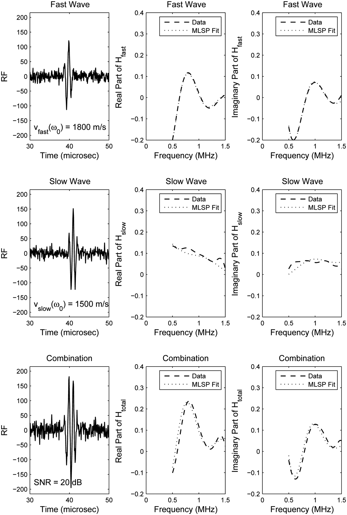
RF signals (left column), real and imaginary parts of H(ω) and MLSP method fits (middle and right columns) for simulated data with vfast(ω0) = 1800 m/s and SNR = 20 dB. The lower middle and lower right graphs show the result of applying the MLSP method directly to Htotal(ω), not merely the sum of the results of applying the MLSP method to Hfast(ω) and Hslow(ω).
Figure 3a shows estimates of fast and slow wave amplitudes as functions of SNR for vfast(ω0) = 2100 m/s using MLSP (*) and maximum-β dual MLSPCF (o) methods. Both methods yielded estimated means that were accurate to within 4% for SNR values ranging from 20 to 50 dB. Variances of estimates decreased as SNR increased. Chirp filtering offered no discernible improvement for amplitude estimation. In this case, there was no meaningful difference between the maximum-β () dual chirp filter (shown) and the conservative chirp filter (not shown).
Figure 3.

The dependence of wave parameter estimates on SNR using MLSP and MLSPCF methods for vfast(ω0) = 2100 m/s (simulation). Dotted lines show true values. a) fast and slow wave amplitudes, b) fast and slow wave attenuation coefficient slopes, c) fast wave phase velocity at 1 MHz, d) slow wave phase velocity at 1 MHz.
Figure 3b shows estimates of fast and slow wave attenuation coefficient slopes as functions of SNR for vfast(ω0) = 2100 m/s using MLSP (*) and maximum-β dual MLSPCF (o) methods. Both methods yielded estimated means that were accurate to within 0.25 dB/cmMHz (4%) for SNR values ranging from 20 to 50 dB. Variances of estimates decreased as SNR increased. Chirp filtering offered no discernible improvement for attenuation coefficient slope estimation. In this case, there was no meaningful difference between the maximum-β dual chirp filter (shown) and the conservative chirp filter (not shown).
Figure 3 shows estimates of fast wave (Figure 3c) and slow wave (Figure 3d) phase velocity at 1 MHz as functions of SNR for vfast(ω0) = 2100 m/s using MLSP (*), conservative MLSPCF (x), and maximum-β dual MLSPCF (o) methods. For SNR ≥ 25 dB, chirp filtering reduced the average fast wave phase velocity bias from about 91 m/s (4.3%) (no filter) to 63 m/s (3.0%) (conservative chirp filter) and 15 m/s (0.7%) (dual chirp filter) and reduced the average slow wave phase velocity bias from about 18 m/s (1.2%) (no filter) to 0.5 m/s (0.1%) (dual chirp filter). Variances of estimates decreased as SNR increased. The chirp filter loses its value for the slow wave phase velocity at SNR < 25 dB because of the high variance of the MLSPCF-based slow wave phase velocity estimate.
Figure 4 shows estimates of fast wave (Figure 4a) and slow wave (Figure 4b) amplitude as functions of true vfast(ω0) using MLSP (*) and maximum-β dual MLSPCF (o) methods. Both methods demonstrated substantial bias for vfast(ω0) ≤ 1700 m/s, i.e. vfast(ω0) − vslow(ω0) ≤ 200 m/s. For vfast(ω0) ≥ 1700 m/s, i.e. vfast(ω0) − vslow(ω0) ≥ 200 m/s, chirp filtering reduced the average amplitude bias from 4.0% to 1.0% (fast wave) and from 12% to 3% (slow wave). Variances of estimates decreased as fast/slow wave velocity differential increased. In this case, there was no meaningful difference between the dual chirp filter (shown) and the conservative chirp filter (not shown).
Figure 4.

The dependence of wave parameter estimates on fast wave phase velocity using MLSP and MLSPCF methods for SNR = 35 dB. (simulation). Dotted lines show true values. a) fast wave amplitude, b) slow wave amplitude, c) fast wave attenuation coefficient slope, d) slow wave attenuation slope, e) fast wave phase velocity at 1 MHz, f) slow wave phase velocity at 1 MHz.
Figure 4 shows estimates of fast wave (Figure 4c) and slow wave (Figure 4d) attenuation coefficient slope as functions of vfast(ω0) using MLSP (*) and maximum-β dual MLSPCF (o) methods. Both methods demonstrated substantial bias for vfast(ω0) < 1700 m/s, i.e. vfast(ω0) − vslow(ω0) ≤ 200 m/s. For vfast(ω0) ≥ 1700 m/s, i.e. vfast(ω0) − vslow(ω0) ≥ 200 m/s, chirp filtering reduced the average attenuation coefficient slope bias from 1.2 dB/cmMHz (6.0%) to 0.7 dB/cmMHz (3.6%) (fast wave) and from 0.6 dB/cmMHz (9.0%) to 0.3 dB/cmMHz (4.8%) (slow wave). Variances of estimates decreased as fast/slow wave velocity differential increased. In this case, there was no meaningful difference between the dual chirp filter (shown) and the conservative chirp filter (not shown).
Figure 4 shows estimates of fast wave (Figure 4e) and slow wave (Figure 4f) phase velocity at 1 MHz as functions of vfast(ω0) using MLSP (*), conservative MLSPCF (x), and maximum-β dual MLSPCF (o) methods. Chirp filtering reduced the average fast wave phase velocity bias from about 73 m/s (3.9%) (no filter) to 48 m/s (2.6%) (conservative chirp filter) and 13 m/s (0.7%) (dual chirp filter) and reduced the average slow wave phase velocity bias from about 19 m/s (1.3%) (no filter) to 3.6 m/s (0.2%) (conservative or dual chirp filter).
B. LDPE / Cancellous-Bone-Mimicking-Phantom Slab Experiment
Figure 5 shows RF signals passing through 100% LDPE (top), 100% cancellous-bone-mimicking-phantom slab (middle), and 50% LDPE / 50% cancellous-bone-mimicking-phantom slab (bottom). Table 1 shows measurements of wave parameters measured on these signals, including conservative MLSPCF method results. Dual MLSPCF-method estimates of wave parameters had higher variances than conservative MLSPCF-method estimates, perhaps because of the considerable variance of the value of MLSP-method estimates of slow wave attenuation coefficient slope (14.1 ± 1.9 dB/cmMHz) used to compute D(ω; ). Chirp filtering reduced the average fast wave phase velocity bias from 100 m/s (5.1%) (no filter) to 69 m/s (3.5%) and reduced the average slow wave phase velocity bias from 29 m/s (1.9%) (no filter) to 10 m/s (0.7%). Chirp filtering did not offer consistent improvement in estimation of attenuation coefficient slopes. Estimates of attenuation coefficient slopes for MLSP and MLSPCF methods were only accurate to within about 1 dB/cmMHz. The accuracies of the MLSP and MLSPCF methods relative to the ranges of values for wave parameters reported for cancellous bone are considered in the Discussion section. The SNR for this experiment (ratio of maximum time-domain pulse amplitude to average time-domain noise amplitude) was measured to be 34.6 ± 1.0 dB.
Figure 5.

RF signals passing through 100% LDPE (top), 100% cancellous-bone-mimicking-phantom slab (middle), and 50% LDPE / 50% cancelloous-bone-mimicking-phantom slab (bottom). The top and middle signals have been offset by 400 and 200 arbitrary units respectively.
Table 1.
A comparison of estimates of fast and slow wave attenuation coefficient slopes and phase velocities in the LDPE / cancellous-bone-mimicking-phantom composite and in the individual media obtained 1) by applying the MLSP and conservative MLSPCF methods on the signal passing through the composite, and 2) by applying log spectral difference (Equation 13) and spectral phase velocity (Equation 14) methods on the signals passing through the individual media.
| Material | Source Signal | Method | Wave | βj (dB/cmMHz) | vj(ω0) (m/s) |
|---|---|---|---|---|---|
| Composite | H total (ω) | MLSP | fast slow |
4.3 ± 1.8 14.1 ± 1.9 |
2045 ± 18 1556 ± 5 |
| Composite | H total (ω) | Conservative MLSPCF |
fast slow |
2.2 ± 1.6 15.6 ± 1.5 |
2014 ± 13 1537 ± 10 |
| LDPE Plate | H fast (ω) | Log Spectral Difference | fast | 3.5 ± 0.1 | - |
| LDPE Plate | H fast (ω) | Spectral Phase Velocity | fast | - | 1945 ± 11 |
| Cancellous Bone Phantom Slab | H slow (ω) | Log Spectral Difference | slow | 15.5 ± 0.2 | - |
| Cancellous Bone Phantom Slab | H slow (ω) | Spectral Phase Velocity | slow | - | 1527 ± 13 |
C. Polycarbonate / Cancellous-Bone-Mimicking-Phantom Experiment
Figure 6a shows experimental estimates of fast wave (polycarbonate) attenuation coefficient slopes as functions of fast wave relative time-domain peak amplitude using MLSP (*) and weighted-average dual MLSPCF (o) methods. The weighted-average dual MLSPCF method estimates (shown in Figure 6) were preferred to the maximum-β estimates (not shown in Figure 6) because of smaller variance. The MLSP method produced substantial bias when the fast wave relative time-domain peak amplitude was less than 10%. Chirp filtering reduced the average fast wave attenuation coefficient slope bias from 0.19 dB/cmMHz (5.9%) to 0.10 dB/cmMHz (3.1%) (dual chirp filter). The SNR for this experiment was measured to be 33.5± 1.0 dB.
Figure 6.

The dependence of wave parameter estimates on wave strength (relative time-domain amplitude) using MLSP and MLSPCF methods (experiment). Dotted lines show values measured on media individually. a) fast wave attenuation slope, b) slow wave attenuation slope, c) fast wave phase velocity, d) slow wave phase velocity.
Figure 6b shows experimental estimates of slow wave (cancellous bone phantom) attenuation coefficient slope as functions of slow wave relative time-domain peak amplitude using MLSP (*), conservative MLSPCF (x), and weighted-average dual MLSPCF (o) methods. For 20% ≤ slow wave relative time-domain peak amplitude ≤ 90%, the average slow wave attenuation coefficient slope bias was 0.27 dB/cmMHz (1.9%) (no filter), 0.26 dB/cmMHz (1.9%) (conservative chirp filter), and 0.30 dB/cmMHz (2.1%) (dual chirp filter). When the slow wave relative time-domain peak amplitude was only 10%, the MLSP method produced a good result, but the conservative and dual MLSPCF methods demonstrated substantial variability and are not shown.
Figure 6c shows experimental estimates of phase velocity at 500 kHz of the fast wave (polycarbonate) as functions of fast wave relative time-domain peak amplitude using MLSP (*) and weighted-average dual MLSPCF (o) methods. Chirp filtering reduced the average fast wave phase velocity bias from 32.8 m/s (1.5%) (no filter) to 16.8 m/s (0.8%) (dual chirp filter).
Figure 6d shows experimental estimates of phase velocity at 500 kHz of the slow wave (cancellous-bone-mimicking phantom) as functions of slow wave relative time-domain peak amplitude using MLSP (*), conservative MLSPCF (x), and weighted-average dual MLSPCF (o) methods. For slow wave relative time-domain peak amplitude ≥ 20%, chirp filtering reduced the slow wave phase velocity bias from 22.6 m/s (1.5%) (no filter) to 17.3 m/s (1.1%) (conservative chirp filter) and to 10.4 m/s (0.7%) (dual chirp filter). However, when the slow wave relative time-domain peak amplitude was only 10%, the conservative MLSPCF method produced a greater bias than the MLSP method, and the dual MLSPCF method demonstrated substantial variability (not shown).
V. DISCUSSION
Pulses transmitted through cancellous bone samples contain important information regarding material and structural properties. This information can be enhanced when pulses are decomposed into fast and slow wave components. This decomposition is often challenging, however, due to temporal overlap between the two components. Previously, the MLSP method was shown to be effective for a broad range of SNR’s and fast/slow phase velocity differentials in simulations and phantom studies designed to mimic the propagation of ultrasound through bovine cancellous bone (Wear, 2010). In the present study, the parameter space was expanded to include a broad range of fast/slow wave time-domain amplitude ratios, which is important because the estimation task becomes more challenging when one wave is has much lower amplitude than the other. In addition, a chirp filter for pre-processing the signal prior to application of the MLSP method was derived and validated.
The three methods (MLSP, conservative MLSPCF and dual MLSPCF) were highly effective over a broad range of amplitudes, attenuation coefficient slopes, and phase velocities but could exhibit degraded performance for low values of fast/slow phase velocity differential (e.g., < 200 m/s), relative wave amplitude (e.g., ≤ 10%), or SNR (e.g., ≤ 20 dB). The MLSPCF methods were not consistently better than the MLSP method for estimates of fast and slow wave amplitudes or attenuation coefficient slopes. The MLSPCF methods (conservative and dual) exhibited significantly lower biases than the MLSP method for phase velocity estimates, except for very low-relative-amplitude waves (e.g., < 10%). For the wave with the smaller of the two attenuation coefficient slopes, the conservative and dual MLSPCF methods yielded identical results (by definition). For the wave with the higher of the two attenuation coefficient slopes, the dual MLSPCF method exhibited significantly lower biases than the conservative MLSPCF method, except for cases of insufficient values of fast/slow phase velocity differential (e.g., < 150 m/s) or wave relative amplitude (e.g., ≤ 10%). Therefore, for cases when the fast wave relative amplitude is near 10% (Nagatani et al., 2008), the chirp filter may not be advisable for fast wave parameter estimation.
Table I shows that the accuracies of the MLSP and MLSPCF methods in the LDPE / cancellous-bone-mimicking phantom slab experiment were on the order of 1 dB/cmMHz for attenuation coefficient slopes. This accuracy is not great but not bad considering the wide range of attenuation coefficient slopes reported for fast waves (bovine: 60 – 102 dB/cmMHz; human: 20 – 140 dB/cmMHz) and slow waves (bovine: 17 – 26 dB/cmMHz; human: 18 – 40 dB/cmMHz) in cancellous bone (Cardoso, et al., 2003). Similarly the accuracies for the MLSP and MLSPCF methods were on the order of 100 m/s and 69 m/s respectively for fast wave phase velocity (at 500 kHz) and 29 m/s and 10 m/s for slow wave phase velocity (at 500 kHz). This accuracy is not great but not bad considering the wide range of phase velocities reported for fast waves (bovine: 1710 – 3500 m/s; human: 1480 – 2900 m/s) and slow waves (bovine: 1175 – 1480 m/s; human: 1210 m/s – 1485 m/s) in cancellous bone (Hosokawa and Otani, 1997; Hughes et al., 1999; Cardoso, et al., 2003; Mizuno et al., 2009). When higher accuracy is required, alternative methods (Marutyan et al., 2007) may be useful but can carry the price of increased complexity and computation time. The Bayesian method (Marutyan et al., 2007) may be particularly valuable for estimation of wave parameters under challenging conditions when the MLSP and MLSPCF methods begin to break down—e.g., low fast/slow wave phase velocity differential, low wave amplitude (relative to the higher-amplitude wave), or low SNR.
Since the MLSP and MLSPCF methods perform functional fits in frequency domain, their performances tend to improve with bandwidth. The MLSP and MLSPCF methods produce estimates of phase velocity only at the reference frequency rather than across the entire frequency band of analysis. Full frequency-dependent phase velocity, if required, may be estimated using Equation 4 and the MLSP- or MLSPCF-method based estimates of attenuation coefficient slope and phase velocities at the reference frequency (ω0).
The values for attenuation coefficient slope and phase velocity in the polycarbonate plate and cancellous-bone-mimicking phantom (Figure 6) differed somewhat from values previously reported (Wear, 2010). Some reasons for the discrepancy may include 1) different samples of polycarbonate were used in the two studies, 2) different cancellous-bone-mimicking phantoms were used in the two studies (although they had the same manufacturer and model), 3) the analysis bandwidth was 200–800 kHz in the present study instead of 200–650 kHz in the previous study, 4) phantoms were somewhat inhomogeneous and measurements varied with exact volume of interrogation, and 5) the temperature of the water was 18.6° in the present study instead of 19.9° in the previous study. In addition, in the present study, the values for attenuation coefficient slope and phase velocity for the cancellous-bone-mimicking phantom (Figure 6) and the cancellous-bone-mimicking phantom slab (Table 1) were somewhat different. Some reasons for the discrepancy may include 1) the slab was cut from an older sample and properties may have drifted with age, 2) the cut surface of the phantom slab was not perfectly planar (because rubber-like materials are difficult to cut), and 3) the phantoms were somewhat inhomogeneous and measurements varied with exact volume of interrogation.
In conclusion, the MLSP and MLSPCF methods are fast and reasonably accurate for estimating amplitudes, attenuation coefficient slopes and phase velocities in two-component pulses but can exhibit degraded performance for insufficient values of fast/slow phase velocity differential, wave relative amplitude. or SNR. The MLSPCF method often exhibits lower bias for phase velocity than the MLSP method.
ACKNOWLEDGEMENTS
The author is grateful to Robert F. Wagner for discussions in the early 1990’s regarding Prony’s method for applications other than ultrasonic characterization of bone. The author is grateful for funding from the FDA Office of Women’s Health. The mention of commercial products, their sources, or their use in connection with material reported herein is not to be construed as either an actual or implied endorsement of such products by the Department of Health and Human Services.
REFERENCES
- Anderson CC, Marutyan KR, Holland MR, Wear KA, and Miller JG, (2008). “Interference between wave modes may contribute to the apparent negative dispersion observed in cancellous bone,” J. Acoust. Soc. Am, 124, 1781–1789. [DOI] [PMC free article] [PubMed] [Google Scholar]
- Anderson CC, Pakula M, Holland MR, Bretthorst GL, Laugier P, and Miller JG, (2009). “Fast and slow wave properties of cancellous bone derived from sonometry measurements using Bayesian inference,” Proc. 3rd Euro. Symp. Ultrason. Char. Bone, Bydgoszcz, Poland, Sept. 17–18, p. 21. [Google Scholar]
- Barkmann R, Laugier P, Moser U, Dencks S, Klausner M, Padilla F, Haïat G, Heller M, and Glüer C, (2008) “In Vivo measurements of ultrasound transmission through the human proximal femur,” Ultrasound Med. & Biol, 34, 1186–1190. [DOI] [PubMed] [Google Scholar]
- Bauer AQ, Marutyan KR, Holland MR, and Miller JG, (2008), “Negative dispersion in bone: the tole of interference in measurements of the apparent phase velocity of two temporally overlapping signals,” J. Acoust. Soc. Am, 123, 2407–2414. [DOI] [PMC free article] [PubMed] [Google Scholar]
- Biot MA (1956a), “Theory of propagation of elastic waves in a fluid saturated porous solid I. Low frequency range,” J. Acoust. Soc. Am. 28, 168–178. [Google Scholar]
- Biot MA (1956b), “Theory of propagation of elastic waves in a fluid saturated porous solid II. High frequency range,” J. Acoust. Soc. Am 28, 179–191. [Google Scholar]
- Biot MA (1956c), “Theory of deformation of a porous viscoelastic anisotropic solid.” J. Appl. Phys, 27, 459–467. [Google Scholar]
- Biot MA (1962), “Generalized theory of acoustic propagation in porous dissipative media,” J. Acoust. Soc. A, 34, 1254–1264. [Google Scholar]
- Biot MA (1963), “Mechanics of deformation and acoustic propagation inporous media,” J. Appl. Phys, 33, 1482–1498. [Google Scholar]
- Breban S, Padilla F, Fujisawa Y, Mano I, Masukawa M, Benhamou CL, Otani T, Laugier P, and Chappard C, (2010). “Trabecular and cortical bone separately assessed at radius with a new ultrasound device, in a young adult population with various physical activities,” Bone, 46, 1620–1625. [DOI] [PubMed] [Google Scholar]
- Cardoso L, Teboul F, Sedel L, Oddou C, and Meunier A, (2003). “In vitro acoustic waves propagation in human and bovine cancellous bone,” J. Bone. Miner. Res, 18, 1803–1812. [DOI] [PubMed] [Google Scholar]
- Cardoso L, Meunier A, and Oddou C, (2008). “In vitro acoustic wave propagation in human and bovine cancellous bone as predicted by Biot’s theory,” J. Mech. Med., Biol, 8, 183–201. [Google Scholar]
- Cowin SC, and Cardoso L, (2010). “Fabric dependence of wave propoagation in anisotropic porous media,” Biomech. Model Mechanobiol, Published online 12 May 2010. http://www.springerlink.com/content/l127584847220211/fulltext.pdf, DOI 10.1007/s10237-010-0217-7last viewed 7/14/10. [DOI] [PMC free article] [PubMed] [Google Scholar]
- Droin P, Berger G and Laugier P, (1998). “Velocity dispersion of acoustic waves in cancellous bone.” IEEE Trans. Ultrason. Ferro. Freq. Cont 45, 581–592. [DOI] [PubMed] [Google Scholar]
- Fellah ZEA, Chapelon JY, Berger S, Lauriks W, and Depollier C, (2004). “Ultrasonic wave propagation in human cancellous bone: application of Biot theory, J. Acoust. Soc. Am, 116, 61–73. [DOI] [PubMed] [Google Scholar]
- Fellah ZEA , Sebaa N, Fellah M, Mitri FG , Ogam E , Lauriks W , and Depollier C, (2008). “Application of the Biot model to ultrasound in bone: direct problem,” IEEE Trans Ultrason, Ferro, and Freq Cont, 55, 1508–1515. [DOI] [PubMed] [Google Scholar]
- Haïat G, Padilla F, Peyrin F, and Laugier P, (2008b). “Fast wave ultrasonic propagation in trabecular bone: numerical study of the influence of porosity and structural anisotropy,” J. Acoust. Soc. Am, 123, 1694–1705. [DOI] [PubMed] [Google Scholar]
- Haire TJ, and Langton CM (1999), “Biot Theory: A review of its application to ultrasound propagation through cancellous bone,” Bone, 24, 291–295. [DOI] [PubMed] [Google Scholar]
- Hosokawa A, and Otani T, (1997). “Ultrasonic wave propagation in bovine cancellous bone,” J. Acoust. Soc. Am, 101, 558–562. [DOI] [PubMed] [Google Scholar]
- Hosokawa A, and Otani T, (1998). “Acoustic anisotropy in bovine cancellous bone,” J. Acoust. Soc. Am, 103, 2718–2722. [DOI] [PubMed] [Google Scholar]
- Hosokawa A (2005). “Simulation of ultrasound propagation through bovine cancellous bone using elastic and Biot’s finite-difference time-domain methods,” J Acoust Soc Am, 118, 1782–1789. [DOI] [PubMed] [Google Scholar]
- Hosokawa A, (2008) “Development of a numerical cancellous bone model for finite-difference time-domain simulations of ultrasound propagation,” IEEE Trans Ultrason, Ferro, Freq Cont, 55, 1219–1233. [DOI] [PubMed] [Google Scholar]
- Hughes ER, Leighton TG Petley GW, and White PR, (1999). “Ultrasonic propagation in cancellous bone: a new stratified model,” Ultrasound Med. & Biol, 25, 811–821. [DOI] [PubMed] [Google Scholar]
- Hughes ER, Leighton TG, Petley GW, White PR, and Chivers RC, (2003), “Estimation of critical and viscous frequencies for Biot theory in cancellous bone,” Ultrasonics, 41, 365–368. [DOI] [PubMed] [Google Scholar]
- Hughes ER, Leighton TG, White PR, and Petley GW, (2007) “Investigation of an anisotropic tortuosity in a Biot model of ultrasonic propagation in cancellous bone,” J. Acoust. Soc. Am, 121, 568–574. [DOI] [PubMed] [Google Scholar]
- Kazmarek M, Kubik J, and Pakula M, (2002). “Short ultrasonic waves in cancellous bone,” Ultrasonics, 40, 95–100. [DOI] [PubMed] [Google Scholar]
- Kaufman JJ, Xu W, Chiabrera AE, and Siffert RS (1995), “Diffraction effects in insertion mode estimation of ultrasonic group velocity,” IEEE Trans. Ultrason. Ferro., Freq. Cont, 42, 232–242. [Google Scholar]
- Kaufman JJ, Luo G, and Siffert RS (2007). “A portable real-time ultrasonic bone densitometer,” Ultrasound Med. Biol, 33, 1445–1452. [DOI] [PMC free article] [PubMed] [Google Scholar]
- Kumaresan R, and Tufts DW (1982). Estimating the parameters of exponentially damped sinusoids and pole-zero modeling in noise, IEEE Trans. Acoust. Speech Signal Process, ASSP-30, 833–840. [Google Scholar]
- Kuc R and Schwartz M (1979) Estimating the acoustic attenuation coefficient slope for liver from reflected ultrasound signals. IEEE Trans Son Ultrason SU-26, 353–362. [Google Scholar]
- Laugier P, (2008) “Instrumentation for In Vivo Ultrasonic Characterization of Bone Strength,” IEEE Trans Ultrason Ferro, Freq Cont, 55, 1179–1196. [DOI] [PubMed] [Google Scholar]
- Le Floch V, McMahon DJ, Luo G, Coeh A, Kaufman JJ, Shane E, and Siffert RS., (2008), “Ultrasound simulation in the distal radius using clinical high-resolution peripheral CT images,” Ultrasound Med. Biol, 34, 1317–1326. [DOI] [PMC free article] [PubMed] [Google Scholar]
- Lee KI, Roh H, and Yoon SW (2003), “Acoustic wave propagation in bovine cancellous bone: Application of the modified Biot-Attenborough model,” J. Acoust. Soc. Am, 114, 2284–2293. [DOI] [PubMed] [Google Scholar]
- Lee KI, and Yoon SW (2006). “Comparison of acoustic characteristics predicted by Biot’s theory and the modified Biot-Attenborough model in cancellous bone, J Biomech, 39, 364–368. [DOI] [PubMed] [Google Scholar]
- Marple SL, (1987). Digital Spectral Analysis with Applications, Englewood Cliffs, NJ, Prentice-Hall Inc., 303–349. [Google Scholar]
- Marutyan KR, Holland MR, and Miller JG (2006), “Anomalous negative dispersion in bone can result from the interference of fast and slow waves,” J. Acoust. Soc. Am, 120, EL55–EL61. [DOI] [PubMed] [Google Scholar]
- Marutyan KR, Bretthorst GL, and Miller JG (2007). “Bayesian estimation of the underlying bone properties from mixed fast and slow mode ultrasonic signals” J. Acoust. Soc. Am, 121, EL8–EL15. [DOI] [PubMed] [Google Scholar]
- McKelvie ML, and Palmer SB (1991), “The interaction of ultrasound with cancellous bone,” Phys. Med. Biol, 1331–1340. [DOI] [PubMed] [Google Scholar]
- Mizuno K, Matsukawa M, Otani T, Laugier P, and Padilla F, (2009), “Propagation of two longitudinal waves in human cancellous bone: An in vitro study,” J. Acoust. Soc. Am, 125, 3460–3466. [DOI] [PubMed] [Google Scholar]
- Mohamed MM, Shaat LT, and Mahmoud AN, (2003), “Propagation of ultrasonic waves through demineralized cancellous bone,” IEEE Trans. Ultrason., Ferro., and Freq. Cont, 50, 279–288. [DOI] [PubMed] [Google Scholar]
- Nagatani Y, Mizuno K, Saeki T, Matsukawa M, Sakaguchi T, and Hosoi H, (2008), “Numerical and experimental study on the wave attenuation in bone – FDTD simulation of ultrasound propagation in cancellous bone,” Ultrasonics, 48, 607–612. [DOI] [PubMed] [Google Scholar]
- Nicholson PHF , Lowet G, Langton CM, Dequeker J, and Van der Perre G, (1996), “Comparison of time-domain and frequency-domain approaches to ultrasonic velocity measurements in trabecular bone,” Phys. Med. Biol, 41, 2421–2435. [DOI] [PubMed] [Google Scholar]
- O’Donnell M, Jaynes ET, and Miller JG, (1981) “Kramers-Kronig relationship between ultrasonic attenuation and pahse velocity,” J. Acoust. Soc. Am, 69, 696–701. [Google Scholar]
- Osborne MR, and Smyth GK, (1995) “A modified Prony algorithm for exponential function fitting,” J. Sci. Comput, 16, 119–137. [Google Scholar]
- Pakula M, and Kubik J, (2002). “Propagation of ultrasonic waves in cancellous bone. Micro and macrocontinual approach,” Poromechanics II, ed. By Auriault JL et al. Swets and Zeitlinger, Lisse, 65–70. [Google Scholar]
- Pakula M, Padilla F, Laugier P, and Kaczmarek M, (2008). “Application of Biot’s theory to ultrasonic characterization of human cancellous bones: Determination of structural, material, and mechanical properties,” J Acoust Soc Am, 123, 2415–2423. [DOI] [PubMed] [Google Scholar]
- Pierce AD, (1981), Acoustics: An introduction to its physical principles and applications. McGraw-Hill, New York, NY, 31. [Google Scholar]
- Riekkinen O, Hakulinen MA, Timonen M, Töyräs J, and Jurvelin JS, (2006), “Influence of overlying soft tissues on trabecular bone acoustic measurement at various ultrasound frequencies,” Ultrasound Med. Biol, 32, 1073–1083. [DOI] [PubMed] [Google Scholar]
- Riekkinen O, Hakulinen MA, Töyräs J, and Jurvelin JS (2008), “Dual-frequency ultrasound—new pulse-echo technique for bone densitometry,” Ultrasound Med. Biol, 34, 1703–1708. [DOI] [PubMed] [Google Scholar]
- Sarvazyan A, Tatarinov A, Egorov V, Airapetian S, Kurtenok V, and Gatt CJ, (2009), “Application of the dual-frequency ultrasonometer for osteoporosis detection,” Ultrasonics, 49, 331–337. [DOI] [PMC free article] [PubMed] [Google Scholar]
- Sebaa N, Fellah ZEA, Fellah M, Ogam E, Mitri FG, Depollier C, and Lauriks W (2008). “Application of the Biot model to ultrasound in bone: inverse problem,” IEEE Trans Ultrason, Ferro, and Freq Cont, 55, 1516–1523. [DOI] [PubMed] [Google Scholar]
- http://Statsci.org. (2010). http://www.statsci.org/, last viewed 3/24/10.
- Strelitzki R, and Evans JA, (1996), “On the measurement of the velocity of ultrasound in the os calcis using short pulses,” Eur. J. Ultrasound, 4, 205–213. [Google Scholar]
- Van Blaricum ML and Mittra R (1975). A technique for extracting the poles and residues of a system directly from its transient response, IEEE Trans. Antennas Propag, AP-23, 777–781. [Google Scholar]
- Waters KR, Hughes M, Mobley J, Brandenburger G, and Miller JG, (2000). “On the applicability of Kramers-Kronig relations for ultrasound attenuation obeying a frequency power law, “ J. Acoust. Soc. Am, 108, 556–563. [DOI] [PubMed] [Google Scholar]
- Waters KR, Mobley J, Miller JG, (2005). “Causality-imposed (Kramers-Kronig) relationships between attenuation and dispersion,” IEEE Trans. Ultrason. Ferro. Freq. Cont, 52, 822–833. [DOI] [PubMed] [Google Scholar]
- Waters KR, and Hoffmeister BK, (2005). “Kramers-Kronig analysis of attenuation and dispersion in trabecular bone,” J. Acoust. Soc. Am, 118, 3912–3920. [DOI] [PubMed] [Google Scholar]
- Wear KA (2000a), “Measurements of phase velocity and group velocity in human calcaneus,” Ultrason. Med. Biol, 26, 641–646. [DOI] [PMC free article] [PubMed] [Google Scholar]
- Wear KA, Laib A, Stuber AP, and Reynolds JC, (2005), “Comparison of measurements of phase velocity in human calcaneus to Biot theory,” J Acoust Soc Am, 117, 3319–3324. [DOI] [PMC free article] [PubMed] [Google Scholar]
- Wear KA, (2010), “Decomposition of two-component ultrasound pulses in cancellous bone using modified least squares Prony’s method—phantom experiment and simulation,” Ultrasound Med. & Biol, 36, 276–287. [DOI] [PMC free article] [PubMed] [Google Scholar]
- Williams JL (1992). “Ultrasonic wave propagation in cancellous and cortical bone: predictions of some experimental results by Biot’s theory,” J. Acoust. Soc. Am, 92, 1106–1112. [DOI] [PubMed] [Google Scholar]