Integration of elicited expert information via a power prior in Bayesian variable selection: Application to colon cancer data

Abstract

Background:

Building tools to support personalized medicine needs to model medical decision-making. For this purpose, both expert and real world data provide a rich source of information. Currently, machine learning techniques are developing to select relevant variables for decision-making. Rather than using data-driven analysis alone, eliciting prior information from physicians related to their medical decision-making processes can be useful in variable selection. Our framework is electronic health records data on repeated dose adjustment of Irinotecan for the treatment of metastatic colorectal cancer. We propose a method that incorporates elicited expert weights associated with variables involved in dose reduction decisions into the Stochastic Search Variable Selection (SSVS), a Bayesian variable selection method, by using a power prior.

Methods:

Clinician experts were first asked to provide numerical clinical relevance weights to express their beliefs about the importance of each variable in their medical decision making. Then, we modeled the link between repeated dose reduction, patient characteristics, and toxicities by assuming a logistic mixed-effects model. Simulated data were generated based on the elicited weights and combined with the observed dose reduction data via a power prior. We compared the Bayesian power prior-based SSVS performance to the usual SSVS in our case study, including a sensitivity analysis using the power prior parameter.

Results:

The selected variables differ when using only expert knowledge, only the usual SSVS, or combining both. Our method enables one to select rare variables that may be missed using only the observed data and to discard variables that appear to be relevant based on the data but not relevant from the expert perspective.

Conclusion:

We introduce an innovative Bayesian variable selection method that adaptively combines elicited expert information and real world data. The method selects a set of variables relevant to model medical decision process.

1. Introduction

Electronic health records (EHR) are used increasingly in hospitals.^1,2 With the development of precision/personalized medicine, medical decision-making has become an increasingly complex process and the use of existing routine data has become essential to design Clinical Decision Support Systems (CDSS). Until now, most CDSS have been knowledge-based systems (also called expert systems since they emulate the decision-making ability of a medical expert). These systems provide explicit algorithms that incorporate reasoning capabilities based on inference engines and knowledge bases, including validated rules, shared guidelines, and ontologies. However, in routine care, medical decision is a quite complex process and all decisions cannot be modelled using knowledge-based models. According to Smellie et al., available guidelines are mostly focused on a particular disease and provide (sometimes very) limited advice for specific patient-centric interpretation.³ Knowledge-based models might not cover all types of situations. In real world, physicians may optimize their medical decision-making process based on multiple patients characteristics and their experience, as they can rely only very partially on guidelines. Therefore, some variables might be taken into account in routine care, while not appearing in knowledge-based models. Consequently, algorithms based on high dimensional routine data analyses are developing in health care, thanks to the increasing performance of data mining and machine learning techniques. For instance, it was already proposed to combine data mining and case-based reasoning for intelligent decision support for pathology ordering by general practitioners.⁴ To apply such methods on routine care data, we have to hypothesize that the variables that influence clinical decisions can be retrieved from the EHR. In selecting relevant variables for use in CDSS, analysis of EHR data may be highly informative. Nevertheless, such routine data analyses also may reflect cognitive bias, such as discrimination.⁵ Moreover, machine learning algorithm-based on EHR data alone may miss rare but important variables, due to a lack of power.

Rather than using either data-driven analysis alone or only expert knowledge to build an algorithm for supporting decision making, a promising alternative is to combine these two types of information. Expert opinion can be incorporated into routine practice data by eliciting from physicians a numerical importance weight of each variable used in their decision making. Thus, if physicians assign a very low weight to some variable, it should not be selected. Concomitantly, if the number of observations does not allow us to detect the effect of a rare variable using only the observed data, then this elicitation could make it possible to reinforce this signal and thus allow the variable to be selected. In this paper, we propose to combine information from EHR data and elicited expert variable importance weights to select a minimal set of relevant variables for use in dose and treatment decisions in the context of multistage chemotherapy.

Building personalized decision support tools to adapt doses in anti-cancer drug regimen is of particular interest since chemotherapy may involve many decisions regarding the choice of drugs and doses. Numerous variables (pharmacogenetic markers, tumor mutations, clinical characteristics) may be involved in the choice of an anti-cancer treatment protocol. Usually, each patient receives his/her first protocol combination dose according to his/her weight, height, age, and biomarkers. During subsequent treatment cycles, variables such as weight loss, ECOG (Eastern Cooperative Oncology Group) performance status, treatment line, response, pharmacogenetic polymorphisms, and toxicities can influence the physicians’ medical decision to either reduce the dose or choose a different treatment line (protocol). Post-hoc analysis of randomized clinical trials and real world data have already highlighted a high frequency of dose adjustment according to patients’ advanced age, and comorbidities such as diabetes, obesity.^6–8 Moreover, some variables may have a known link to certain toxicities.⁹ Therefore, physicians must adapt doses and schedules over consecutive treatment cycles by considering all characteristics of the patient and past treatment lines, doses, and outcomes. Thus, decisions are personalized, and usually only a few observations for a given set of characteristics are available in routine data. Consequently, using data-driven strategies, rare variables that are very important for medical decisions might not be selected.

Because of the large number of variables in an EHR dataset, to select variables relevant for medical decision making, one can use penalization criteria such as bridge, Lasso, SCAD, LARS, elastic net, or OSCAR regressions.^10–14 In the Bayesian setting, Mitchell and Beauchamp have suggested a method based on “spike and slab” priors,¹⁵ with its extension, the Stochastic Search Variable Selection (SSVS) method, that use a mixture of two normal distributions centered on zero, but with different variances as proposed by George and McCulloch.¹⁶ The Bayesian approach can also enable us to incorporate prior expert information.

To combine information from EHR data and expert opinion, we propose using a power prior. Traditionally, power prior methods are used to combine historical data with current data via an informative prior, called the power prior, using Bayesian regression.¹⁷ The power prior parameter allows one to tune how much historical information should be used in posterior estimation of the model parameters. If the power prior parameter is equal to zero, then no historical information is used, and the prior distribution is taken as non informative. If the power prior parameter is equal to one, then all the informative prior distribution is used to compute the posteriors.

Our motivating application is based on observed data derived from an EHR of colorectal cancer patients treated with Irinotecan. Our expert data were obtained from six digestive oncologists by quantifying their subjective importance of variables used in their own decision making. In our proposed method, historical data are replaced by simulated data. The general steps of how we applied the methodology to our motivating application are as follows:

1. First, we independently asked six clinicians who are experts in treating colorectal cancer to specify covariates and numerical clinical relevance weights to reflect their opinions about the importance of each covariate in their decision making. When a covariate takes on a particular value, a clinician will decrease the dose with a probability that relies on the expert’s clinical relevance weights given to this variable. Each clinician gave their own clinical relevance weights linked to each grade of each toxicity type and each level of each covariate.

2. Next, we formulated a Bayesian model for the observed data D, including a spike-and-slab prior to facilitate variable selection using SSVS.

3. We generated a simulated data set D₀ using the clinical relevance weights, and we formulated a synthetic likelihood L(θ|D₀).

4. We used a power prior to combine the usual noninformative prior π₀(θ) with the synthetic likelihood L(θ|D₀) to obtain the prior we actually used. The proposed method combines the physician weights in the posterior as a function of estimated values from the observed data and the elicited weights.

The remainder of the article is organized as follows. In section 2, we describe the case study of patients treated with Irinotecan for colorectal cancer. The proposed methodology is presented formally in section 3. We present the results of our application of the method to the clinical practice data in section 4, and we discuss them in section 5. We close with conclusions in section 6.

2. Case study

To ensure complete reporting of our routinely collected health data, we followed the RECORD statement.¹⁸

2.1. Patient selection

The chemotherapy data analyzed herein were extracted from the patient EHR and stored in an i2b2 clinical data warehouse together with all other hospital health records.^19,20 These data warehouses have been established to facilitate health care data reuse for research. We selected data from the Georges Pompidou University Hospital (HEGP) i2b2 data warehouse, on patients treated for metastatic colorectal cancer who received at least once a combination of drugs, including Irinotecan at a theoretical dose of 180 mg/m² and a theoretical chemotherapy cycle of 14 days, between the 1 July 2003 and 10 November 2017. Selected patients were then split into two samples, one (hereafter called sample 1) with patients having at least one cycle with complete information, and the other (hereafter called sample 2) with patients not fulfilling this criterion.

2.2. Cycle selection

For sample 1, if the patient experienced a dose reduction (dose less than 150 mg/m²) on a cycle with complete observation, we extracted the maximal number of consecutive cycles that included this cycle. Otherwise, we extracted the maximal number of consecutive cycles with complete observation. This procedure offers the opportunity to enrich our sample of patients with dose reductions.

For sample 2, we kept the maximal number of consecutive cycles with less than u missing data by cycle for u ∈ {1, . . . , 10}.

2.3. Variable extraction

Chemotherapy protocols and prescriptions are defined in the Chimio^® (Computer Engineering) software that is used by clinicians for prescription. This software manages the dates of administration for each cycle, the doses of the different drugs, and dose reductions, among others. Some clinical data are also stored by clinicians in Chimio^®, such as body surface area or creatinine clearance.

The screens of the Chimio^® application were reviewed to determine the relevant items to upload into the i2b2 data warehouse.

A total of 1.4 million observations were included from Chimio^® in i2b2, involving 14,000 patients. 1.300 i2b2 concepts were created to store these observations.

To obtain clinical data associated with each chemotherapy cycle, a questionnaire was designed in 2012 at the HEGP to collect the clinical information needed for patient follow-up and dose adjustments. In particular, it contains the toxicities of chemotherapies at each cycle, by organ, graded for severity according to the Common Terminology Criteria for Adverse Events (CTCAE) v4.03 nomenclature. We extracted these toxicities along with other relevant variables (age, ECOG performance status, bilirubin, weight, treatment line) and included laboratory values (neutrophils, platelets, hemoglobin) available in our clinical data warehouse (cf. Table 1).

Table 1.

Definitions of neutropenia, thrombopenia, and anemia.

Toxicities		Grades
		1	2	3	4
Neutropenia	Neutrophils (/mm3)	<2000	<1500	<1000	<500
Thrombopenia	Blood platelets (/mm3)	<150,000	<75,000	<50,000	<25,000
Anemia	Hemoglobin (g/dL)	<12	<10	<8	<6.5

If several clinical reports were available for one cycle, we used the maximal grade for each toxicity variable. We derived the following relevant variables from the clinical report:

• Age < or ≥80 years;

• Weight loss < or ≥10%, since the start of treatment;

• Bilirubin categorized as < 35 μmol/L, between 35 and 50 μmol/L, or ≥ 50 μmol/L;

• Treatment line < 3, = 3 or > 3;

• ECOG performance status and toxicities graduated integer values from 0 (no side effect) to either 3 or 4 (most severe).

2.4. Weight elicitation

Let n be the number of patients and K_i be the number of cycles for patient i ∈ {1, . . . , n}. For each i and k ∈ {1, . . . , K_i}, let x_i,k be the J-vector of variables at the beginning of cycle k. Let $x_{j,c}^{\prime }$ be the value for the cth category of the jth variable, j ∈ {1, . . . , J}, c ∈ {0, . . . , C_j} where C_j + 1 is the number of categories of this variable. Let z_i,k be the L-vector $\left(L={\sum }_{j=1}^J{C}_j\right)$ of all individual variables in x_i,k, where each x_i,k,j is split into C_j dummy variables, each taking a value of 1 if the corresponding category was in x_i,k,j and 0 otherwise.

For each variable j ∈ {1, . . . , J} and each of its possible values c ∈ {1, . . . , C_j}, each physician was asked to specify the clinical relevance weights w_j = (w_j,1, . . . , w_j,Cj ). These weights quantify the importance of variables in dose adaptation decision-making based on individual clinician experience. The minimal and maximal possible values for the weights were restricted to 0 (no severity) and W_max = 100 (the highest possible severity), since this scale is easily understandable by oncologists, and ordered as follows: 0 = w_j,0 ≤ w_j,1 ≤ · · · w_j,Cj ≤ W_max = 100, such that lower grades are less involved in the dose reduction decision than higher grades. For each variable j, w_j,0 = 0 is the weight for the reference level $x_{j,0}^{\prime }$. Similarly, for c ∈ {1, . . . , C_j}, w_j,c is the weight used when the variable x_i,k,j takes the value $x_{j,c}^{\prime }$. For instance, the vector w₇ = (0, 20, 80) is the vector of weights for the 7th variable at its C₇ = 3 levels (the reference level is not included). By analogy with z, w* denotes the L-vector of all clinical relevance weights. This notation follows Bekele and Thall,²¹ in which elicited toxicity severity weights were used to build a score called the “total toxicity burden” for use in adaptive dose-finding.

Table 2 presents the clinical relevance weights elicited from each clinician for each covariate. For example, {0, 20, 80} in the first column (physician 1), in the row “nausea” refers to clinical relevance weights given by physician 1 for grades {1, 2, 3}. The table suggests that the clinician 2 assigned a weight of 20 to a weight loss of more than 10% in his/her decision making, while clinician 4 assigned a weight of 80.

Table 2.

Clinical relevance weights for each covariate elicited from each physician.

Variables	Physicians
				1				2				3
Age ≥80 years	100	–	–	–	60	–	–	–	100	–	–	–
Weight loss > 10%	50	–	–	–	20	–	–	–	50	–	–	–
ECOG performance status (1,2,3,4)	0	20	20	20	0	0	40	100	0	0	80	100
Bilirubin >35, >50 μmol/L	100	100	–	–	40	80	–	–	100	100	–	–
Treatment line 3, >3	30	50	–	–	0	0	–	–	0	0	–	–
Toxicity grades 1, 2, 3, 4
Vomiting	0	20	80	90	0	30	70	100	0	10	10	10
Nausea	0	20	80	–	0	10	50	–	0	10	10	–
Diarrhea	0	40	80	100	0	20	50	100	0	50	80	100
Asthenia	10	50	100	–	10	10	40	–	0	0	70	–
Neutropenia	0	70	100	100	0	0	30	50	0	0	50	50
Thrombopenia	40	100	100	100	0	0	20	30	0	0	50	50
Anemia	0	50	80	100	0	0	20	30	0	0	0	0
	Physicians
Variables				4				5				6
Age ≥80 years	80	–	–	–	100	–	–	–	100	–	–	–
Weight loss > 10%	80	–	–	–	50	–	–	–	60	–	–	–
ECOG performance status (1,2,3,4)	0	20	80	100	0	30	100	100	0	70	100	100
Bilirubin >35, >50 μmol/L	20	80	–	–	100	100	–	–	100	100	–	–
Treatment line 3, >3	0	0	–	–	0	0	–	–	0	50	–	–
Toxicity grades 1, 2, 3, 4
Vomiting	10	20	80	100	0	30	70	100	0	0	70	100
Nausea	10	30	80	–	0	10	40	–	0	0	30	–
Diarrhea	0	20	70	90	0	20	50	100	0	50	100	100
Asthenia	10	50	70	–	0	20	50	–	0	40	80	–
Neutropenia	0	20	70	80	0	0	20	100	0	0	0	50
Thrombopenia	0	50	80	100	0	0	20	70	0	0	0	0
Anemia	0	20	50	70	0	0	30	80	0	0	0	0

3. Methods

In the following section, we introduce the Bayesian mixed model framework, explain how we integrate the elicited expert weights into the statistical model, and describe criteria to assess predictive performance and variable selection.

3.1. Bayesian mixed model framework

We use a mixed-effects logistic regression model where the dose reduction for patient i in cycle k is denoted by the binary variable r_ik, and the covariate vector z_i,k includes patient characteristics and toxicities, updated from the previous cycle

$$\begin{array}{l}\hfill r_{i,k}~\mathcal{B}(p_{i,k}^r)\hfill \\ \mathrm{logit}(p_{i,k}^r)={\theta }_0+{\mathit{\theta }}^T{\mathit{z}}_{i,k}+{\gamma }_i\hfill \\ \hfill {\gamma }_i\stackrel{iid}{~}\mathcal{N}\left(0,{\sigma }_{\gamma }^2\right)\hfill \end{array}$$

where (θ₀, θ) is the L-vector of fixed coefficients, γ_i is the random patient effect, and $\mathcal{B}\left(p^r\right)$ represents the Bernoulli distribution with a probability of success equal to p^r.

For l ∈ {1, . . . , L}, let I_l to be the selection indicator variable as follows

$$I_l=\{\begin{array}{ll}1\hfill & {\text{if}\text{z}}_{\mathrm{..1}}\text{is}\text{in}\text{the}\text{model}\hfill \\ 0\hfill & \text{otherwise}\hfill \end{array}$$

where z_..l is the lth variable. We perform variable selection using the Stochastic Search Variable Selection (SSVS) method, which assumes that θ_l|I_l, l ∈ {1, . . . , L} follows a mixture of two normal distributions, both centered on 0 but with different variances: the first variance is chosen to be small so that unselected variables have estimated coefficients that are very likely to be close to 0, and the second is chosen to be large so that estimated coefficients linked to selected variables can assume a wide range of real values with nontrivial probability.¹⁶ Formally, the distribution of θ_l|I_l, l ∈ {1, . . . , L} is assumed to be

$${\theta }_l\mid I_l~\left(1-I_l\right)T\mathcal{N}\left(0,{\tau }^2\right)+I_{l}T\mathcal{N}\left(0,g{\tau }^2\right)$$ (1)

where (τ, g) are variance parameters, the selection variable indicator I_l follows a Bernoulli distribution with parameter p_l, and $T\mathcal{N}$ is the truncated normal distribution on (−∞, 0]. The truncated normal distribution restricts parameters to negative values, such that the model only accounts for dose reductions. In practice, doses specified per protocol are possibly decreased but not increased. Therefore, there were no dose increases in our data.

3.2. Integration of expert elicitation weights into the power prior method

In this section, we describe how we combined the elicited expert weights with the observed data when modeling dose reductions.

The power prior (PP) method provides a basis for integrating information contained in historical data into a Bayesian analysis,¹⁷ while calibrating the weight of the historical data relative to the current data. In our proposed method, historical data are replaced by simulated data generated using patients with incomplete data (sample 2). For this dataset, we first (1) imputed missing values at random according to the variable distribution in the initial data set and (2) generated dose reductions r₀ according to the elicited weights.

Two alternative approaches were used to generate simulated dose reductions r₀ according to the experts’ elicited weights:

• Approach 1:

  $$r_{0,i^{\prime },k^{\prime }}^{(1)}=\{\begin{array}{ll}1\hfill & \text{if}{\mathit{w}}^{*\text{T}}{\mathit{z}}_{0,{\text{i}}^{\prime },{\text{k}}^{\prime }}>{\text{Q}}_0\hfill \\ 0\hfill & \text{otherwise}\hfill \end{array}$$ (2)
• Approach 2:

  $$\begin{array}{l}{r}_{0,i^{\prime },k^{\prime }}^{(2)}~\mathcal{B}\left(p_{0,i^{\prime },k^{\prime }}^r\right)\\ \mathit{logit}\left(p_{0,i^{\prime },k^{\prime }}^r\right)=-Q_0+{\mathit{w}}^{*T}{\mathit{z}}_{0,i^{\prime },k^{\prime }}\end{array}$$ (3)

In both approaches, Q₀ is a threshold defined to obtain a proportion P₀ of dose reductions, in which Q₀ is the quantile corresponding to the probability 1 − P₀ of the sample made up of ${\left({\mathit{w}}^{*T}{\mathit{z}}_{0,i^{\prime },k^{\prime }}\right)}_{i^{\prime },k^{\prime }}$. Equations (2) and (3) show how the elicited weights were used as covariate parameters in the synthetic data simulation model. Furthermore, the simulated data set depends on the P₀ value that is chosen based on a sensitivity analysis, described in section 3.4. The second approach introduces uncertainty into the dose reduction and makes the process of decision making more similar to that of clinicians in clinical practice by sometimes discarding important variables.

The simulated data are combined with observed data using the PP. This prior is defined as the product of the weighted likelihood of θ conditional on the simulated data and a noninformative prior distribution

$$\pi \left(\mathit{\theta }\mid {\mathit{D}}_0,a_0\right)\propto L{\left(\mathit{\theta }\mid {\mathit{D}}_0\right)}^{a_0}{\pi }_0(\mathit{\theta })$$

where D₀ = (n₀, r₀, z₀) are the simulated data, L(θ|D₀) is the likelihood of θ conditional on the simulated data, 0 ≤ a₀ ≤ 1 is the scale parameter that controls the amount of weight assigned to the simulated data, and π₀(θ) is a noninformative prior for θ.

The posterior distribution of θ is

$$\begin{gathered} \pi \left(\mathit{\theta }\mid \mathit{D},{\mathit{D}}_0,a_0\right)\propto L(\mathit{\theta }\mid \mathit{D})\pi \left(\mathit{\theta }\mid {\mathit{D}}_0,a_0\right) \\ \propto L(\mathit{\theta }\mid \mathit{D})L{\left(\mathit{\theta }\mid {\mathit{D}}_0\right)}^{a_0}{\pi }_0(\mathit{\theta }) \end{gathered}$$

where D = (n, r, z) are the observed data and L(θ|D) is the likelihood of θ conditional on the observed data.

3.3. Bayesian model averaging (BMA)

To combine the weights elicited from different physicians, c ∈ {1, . . . , C}, we use Bayesian Model Averaging (BMA) with the predictive distribution of a coefficient θ_l, l ∈ {1, . . . , L}, which is a weighted average of the posterior distributions of θ_l using our model M_c for each clinician c²²

$$\mathbb{P}\left({\theta }_l\mid \mathit{D}\right)=\sum _{c=1}^C\mathbb{P}\left(M_c\mid \mathit{D}\right)\mathbb{P}\left({\theta }_l\mid M_c,\mathit{D}\right)$$

where the weights $\mathbb{P}\left(M_c\mid \mathit{D}\right)$ are the posterior probabilities of each model

$$\mathbb{P}\left(M_c\mid \mathit{D}\right)=\frac{\mathbb{P}\left(\mathit{D}\mid M_c\right)\mathbb{P}\left(M_c\right)}{{\sum }_{c_1=1}^C\mathbb{P}\left(\mathit{D}\mid M_{c_1}\right)\mathbb{P}\left(M_{c_1}\right)}$$

The marginal likelihood of the model M_c is

$$\mathbb{P}\left(\mathit{D}\mid M_c\right)=\int \mathbb{P}\left(\mathit{D}\mid {\theta }_l,M_c\right)\mathbb{P}\left({\theta }_l\mid M_c\right)\text{d}{\theta }_l$$

where $\mathbb{P}\left(\mathit{D}\mid {\theta }_l,M_c\right)$ is the likelihood and P(θ_l|M_c) is the prior distribution. The expected value and variance of θ_l are given by

$$\{\begin{array}{l}\mathbb{E}\left({\theta }_l\mid \mathit{D}\right)=\sum _{c=1}^C{\widehat{\theta }}_l^c\mathbb{P}\left(M_c\mid \mathit{D}\right)\hfill \\ \mathbb{V}\left({\theta }_l\mid \mathit{D}\right)=\sum _{c=1}^C[\mathbb{V}\left({\theta }_l\mid \mathit{D},M_c\right)+{\left({\widehat{\theta }}_l^c\right)}^2]\mathbb{P}\left(M_c\mid \mathit{D}\right)-E{\left({\theta }_l\mid \mathit{D}\right)}^2\hfill \end{array}$$

where $\widehat{{\theta }_l^c}=\mathbb{E}\left({\theta }_l\mid \mathit{D},M_c\right)$.

3.4. Prior parameter settings

Numerical values of prior hyperparameters g and τ² in equation (1) must be specified so that if ${\theta }_l~\mathcal{N}\left(0,{\tau }^2\right)$, θ_l then estimate ${\widehat{\theta }}_l$ will be close to 0, and if ${\theta }_l~\mathcal{N}\left(0,g{\tau }^2\right)$, then ${\widehat{\theta }}_l$ may take on nonzero real values. In the following, based on a preliminary sensitivity analysis, we chose τ = 1 and g = 100 following the proposal in George and McCulloch.¹⁶ We also took p_l = 0:5, so that all variables have the same probability of being selected by the algorithm. The intercept θ₀ and the covariance of the random effects ${\sigma }_{\gamma }^2$ were assumed to follow a normal distribution with a mean of 0 and variance of 100, and an inverse-gamma distribution with shape and scale parameters equal to 1 and 1, respectively.

For the PP, we performed a sensitivity analysis of prediction performance and variable selection. Two alternative approaches were used to generate the simulated dose reductions r₀ according to the elicited expert weights. We considered the power prior parameter values (a₀ ∈ {0:1, 0.5, 1}), simulated sample sizes (n₀ = n₁, n₀ = 1.77 × n₁), and dose reduction frequencies (P₀ ∈ {2P, P, P/2}).

3.5. Assessment of predictive performance and variable selection

To assess the performance and variable selection, we randomly split the sample with complete observations into two subsets, one for training (70%) and one for performance estimation (30%), and repeated this 10 times, resulting in 10 use cases. Parameters were estimated for each training sample considered as observed data in the likelihood, with variable selection performed on the training sample. For each variable, we counted the proportion of times this variable was selected. Predictive performance then was estimated for each test sample. To assess the model predictive performance, we used the Receiver Operating Characteristic (ROC) curve and its corresponding Area Under the Curve (AUC).

We performed the analyses using R software 3.3.2 version and package R2jags (0.5–7 version). In R2jags, three chains and a burn-in of 1000 were used to implement autojags, combined to Gelman and Rubin’s potential scale reduction factor Rhat = 1.1 as a convergence criterion. The scripts are available from the corresponding author.

4. Results

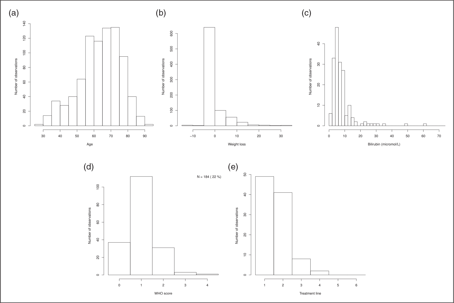
Among the 678 patients in the sample, n = 303 had complete observations over all cycles (sample 1; see Table 3, Figures 1 to 3 for descriptions). There were very few observations with grade 3 or 4 toxicities. Among patients with complete observations over all their cycles, 85 had dose reductions, corresponding to 13% of the observed dose reductions in sample 1.

Table 3.

Covariates for patients with complete observations over all cycles (sample 1).

Variables	0	1	2	3	4
Age ≥80 years	604 (95)	32 (5)	–	–	–
Weight loss > 10%	631 (99)	5 (1)	–	–	–
ECOG performance status	123 (19)	381 (60)	100 (16)	11 (2)	21 (3)
Bilirubin >35, > 50 μmol/L	630 (99)	1 (0)	5 (1)	–	–
Treatment line 3, >3	547 (86)	46 (7)	43 (7)	–	–
Toxicity grades Vomiting	567 (89)	54 (8)	13 (2)	2 (0)	–
Nausea	344 (54)	226 (36)	60 (9)	6 (1)	–
Diarrhea	363 (57)	218 (34)	49 (8)	6 (1)	–
Asthenia	97 (15)	368 (58)	150 (24)	21 (3)	–
Neutropenia	444 (70)	111 (17)	67 (11)	9 (1)	5 (1)
Thrombopenia	524 (82)	104 (16)	6 (1)	1 (0)	1 (0)
Anemia	343 (54)	257 (40)	36 (6)	–	–

Note: Percentages are shown in parentheses.

Figure 1.

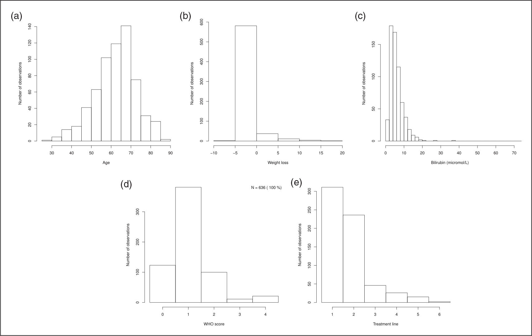
Distribution of age, weight loss, bilirubin, ECOG performance status and treatment line for the n patients with complete observations over all cycles (sample 1). (a) Age; (b) weight loss; (c) Bilirubin; (d) ECOG performance status; and (e) treatment line.

This sample of 303 patients was used as observed data in the method. Thus, 10 training samples of n₁ = 212 patients and 10 validation samples of 91 patients were built to assess the predictive performance of the proposed model. The 375 patients with incomplete data (sample 2) from the initial data set were used to build the simulated dataset by (1) imputing their missing values at random according to the variable distribution in the initial data set and (2) generating dose reductions according to the elicited weights (see Appendix 2 for description of this sample). A flowchart summarizing the use of the data is presented in Figure 4.

The elicitation weights showed that important variables for decision making were the ECOG performance status, except for physician 1, and grade 4 toxicities. Some variables were considered important less consistently, such as the treatment line or anemia. The elicited weights suggest that the six clinicians might act differently when dealing with the same clinical situation.

4.1. Prediction performance

Let P be the proportion of observed dose reductions in each of the 10 training datasets of sample 1. Table 4 summarizes the number of selected variables and AUCs for usual SSVS and SSVS using the PP model with a₀ ∈ {0.1, 0.5, 1}, BMA, and several values of P₀ and n₀. The AUCs did not change with the introduction of a PP, regardless of the parameters considered.

Table 4.

Number of selected variables and AUCs for usual SSVS and SSVS using the power prior for the two approaches, a₀ ∈ {0.1, 0.5, 1}, BMA and several values of P₀ and n₀.

		Number of selected variables			AUC
		SSVS
		5			0.69 (0.04)
		PP – Approach 1
		a0 = 0.1	a0 = 0.5	a0 = 1	a0 = 0.5	a0 = 0.5	a0 = 1
P0 = P	n0 = n1	3	6	9	0.68 (0.03)	0.68 (0.04)	0.68 (0.05)
P0 = P	n0 = 1.77n1	3	6	10	0.68 (0.03)	0.68 (0.04)	0.68 (0.04)
P0 = 2P	n0 = n1	2	8	13	0.69 (0.03)	0.68 (0.04)	0.68 (0.04)
P0 = 2P	n0 = 1.77n1	2	10	14	0.69 (0.04)	0.69 (0.05)	0.69 (0.05)
P0 = P/2	n0 = n1	3	6	11	0.69 (0.03)	0.69 (0.04)	0.68 (0.04)
P0 = P/2	n0 = 1.77n1	2	4	9	0.68 (0.03)	0.68 (0.04)	0.68 (0.03)
		PP – Approach 2
		a0 = 0.1	a0 = 0.5	a0 = 1	a0 = 0.1	a0 = 0.5	a0 = 1
P0 = P	n0 = n1	3	4	9	0.68 (0.03)	0.68 (0.04)	0.69 (0.05)
P0 = P	n0 = 1.77n1	2	4	10	0.68 (0.03)	0.68 (0.05)	0.68 (0.05)
P0 = 2P	n0 = n1	2	6	13	0.69 (0.03)	0.68 (0.04)	0.69 (0.05)
P0 = 2P	n0 = 1.77n1	2	7	13	0.69 (0.03)	0.69 (0.05)	0.69 (0.05)
P0 = P/2	n0 = n1	2	4	10	0.69 (0.03)	0.68 (0.04)	0.69 (0.04)
P0 = P/2	n0 = 1.77n1	3	4	9	0.69 (0.03)	0.68 (0.03)	0.68 (0.03)

4.2. Variable selection

For approach 1 that is used to generate simulated dose reductions, Figures 5 and 6, respectively, show the proportion of times where each variable is selected by the models and the proportion of times where each variable is selected by the models against values of mean weight elicited by clinicians. Figures 7 and 8 are the corresponding figures for approach 2. Tables 5 to 10 in Appendix 1 are the detailed results for all scenarios.

SSVS selects only a few variables. Only five variables were selected at least for five of the 10 cases conducted: bilirubin greater than 35 μmol/L and greater than 50 μmol/L, diarrhea of grade 2 and 3, and anemia of grade 2.

Variable selection varies according to the different settings for the power prior, more particularly with the power prior parameter. Variable selection did not change significantly with a varying sample size and dose reduction frequency of the simulated sample. When using the power prior approach, variables selected by the SSVS were also selected at least for five of the 10 experiences conducted, except anemia grade 2, for which the mean and maximal value for the elicited weights were, respectively, 12 and 50 with four out of the six physicians having chosen a null value for this variable.

For a small value of the power prior parameter, variables having high elicited weights were not selected in more than half of the cases. The number of selected variables with high elicited weights increased with the power prior parameter value. The power prior selects variables with high elicited weight and few observations, such as ECOG performance status grade 3 (11 observations) and vomiting grade 3 (2 observations). It also selects variables with high elicited weight but with a larger number of observations: ECOG performance status grade 4 (21 observations), asthenia grade 3 (21 observations) and age greater than 80 years (32 observations).

5. Discussion

Our method improves SSVS variable selection by automatically selecting relevant variables based on experts’ everyday practice and discarding variables elicited by experts as not being important. Our method was also able to select rare variables that could not be selected using conventional data-driven approaches with relatively small samples. Of note AUC did not significantly vary across the different models and was moderate.

5.1. An automated and flexible variable selection approach

Once expertise is quantified by the elicited weights, our proposed method allows one to automatically select variables without the need for a consensus step. The two suggested approaches for generating simulated data based on experts’ elicitation weights can provide different sets of selected variables, which may be explained by the randomness of the second approach in comparison to the first. Therefore, our method allows to incorporate elicitation variability in several ways and therefore can aggregate multiple expert opinions while taking into account their variability.

The number of variables included in the final model is flexible as it depends heavily on the numerical power prior parameter value, with 2 to 14 among 32 variables selected. Smaller values of the power prior parameter lead to fewer variables selected and discarding variables that were retrieved in the data-driven based analysis (SSVS). Larger values of this parameter lead to a larger number of selected variables combined both data and expert knowledge. Most of the SSVS selected variables were included, except anemia, for which the elicited weights were very low (mean weight: 33). Of note, bilirubin was selected as UGT1A1 polymorphism, closely linked to bilirubin level that is largely described as associated with Irinotecan adverse events.²³ The selected variables were strongly correlated with the elicited weights, with the variables having the highest elicited weight all included when using the largest power prior parameter. Consequently, we suggest repeating the procedure using several different values of the power prior parameter, such as a₀ ∈ {1, 0.5, 0.1}. On this basis, a₀ can be chosen according to the number of relevant variables that one wishes to keep for building a decision tool, or guided by a trade-off between the selected variables stemming from the data and from the elicited expert knowledge.

5.2. An innovative approach to model medical decision

To our knowledge, power prior methods have been used mainly to vary the weight of historical data used in a current data analysis.¹⁷ In this paper, we suggested to use a power prior to incorporate information in the form of clinical expertise by using simulated data obtained from elicited weights. This methodology appears promising and can be applied to a variety of situations involving medical decision making.

The proposed method aimed to model decision making. Personalized medicine requires the consolidation of knowledge about personalized medicine and the development of CDSS that provide actionable information.² Besides knowledge about disease subtypes and genomic variants, comprehensive understanding of the cognitive processes and parameters that influence medical decisions is needed. IT solutions must be proposed for data sharing and building a consensus on clinical interpretations of complex patient data. These solutions could integrate data reasoning capabilities together with computational data-driven approaches like prediction tools, federated queries, and follow-up systems. Not surprisingly, our results show that the clinicians that participated in our study might act differently when dealing with the same clinical situation. Conventional knowledge-based CDSS and guidelines implementation in EHR systems are means to reduce variability in decision making. Our approach is an attempt to make explicit the parameters that influence clinical decisions about dose reduction in cancer treatment and explain data heterogeneity.

5.3. Elicitation step enables to capture practice variability

Predictive performance was moderate with an AUC of approximatively 0.7 for all power prior parameters, which did not change with the addition of expert information. Two phenomena might explain this moderate performance: missing variables and practice variability among physicians. The 32 variables included in our study as potentially important for clinicians’ decisions were those from the follow-up questionnaire used routinely to assign patients’ doses. This assignment is performed the day before the patient venue for organizational purpose, based on this questionnaire. When the six clinicians who elicited their decision process in this study were asked about other variables not in the questionnaire that could influence doses, only two additional variables were mentioned: therapeutic objective (two clinicians) and intestinal obstruction (one clinician). Therefore, it is unlikely that important variables were not included in our study. By contrast, elicited weights deeply vary across physicians, in favor of practice variability among physicians. A study already concluded that large differences observed in practice probably result mostly from individual variation in clinical practice.³ Therefore, the moderate performance achieved by our model is likely due to practice variability and this might hold for most use cases.

5.4. An approach limited by the contain of EHR

Our use case is based on monocentric data. It is indeed very difficult to gather real-world multicentric clinical data such as diarrhea, and vomiting grades due to the lack of interoperability of the different EHR across hospitals for clinical variables. Most multicentric real world data are based on administrative claims that do not contain all relevant information to model medical decision. As a perspective, it is of utmost importance to rely on interoperable EHR to have large sample size. Moreover, EHR contain is limited: it is noteworthy that medical decision process to reduce the dose is not described in EHR, that is, variables used for individual dose reduction are not reported.

5.5. The final perspective: dose regimen modeling to improve survival

Modeling dose regimen is an important intermediate step to model the complex relationship between patients and tumors characteristics, treatment and disease free survival. Indeed, the final aim of our approach is to assess which combination of dose will provide for each patient the best survival. Literature about the relevance of dose adjustment to improve survival is contradictory with some studies showing that reductions decrease survival while other shows no consequence on survival with reduced adverse events.^8,24 Finally, all of a patient’s previous treatments and side effects may be considered by a physician to adapt the dose, not only those in the most recent cycle. Moreover, the time intervals between successive doses vary between patients, depending on their most recent toxicities, although time was not included in our analysis. Furthermore, past doses and administration schedules are major causes of toxicities, so there may be a complex causal effect, which has still to be modelled. While some real world studies highlighted strong difference in chemotherapy use, high frequency of dose adjustment and differential survival compared to clinical trials, no study tackled the complex relationship between dose adjustment and survival.^25,26 Few studies indeed focus on medical decision, and more particularly on dose regimen in routine data model building. This is, however, an essential step to assess drug efficacy. As a perspective, one should develop models that can take into account all these complex steps with the aim to find the best treatment for each patient.

6. Conclusion

In this article, we proposed a Bayesian method based on a power prior approach that allows one to combine information from patient data and elicited expert opinion when performing variable selection. In this method, theoretical doses are generated based on the experts’ elicited weights for variables, with a power prior to analyze the observed data and a simulated dataset based on the weights. Our application shows that this method enables one to select rare variables that cannot be selected using only patient data and to discard variables that appear to be relevant based on the data but not from the expert perspective. Combining expert opinion and data driven knowledge is a crucial step toward personalized medicine. Selection of the optimal set of important variables making in dose reduction decisions is essential to build decision-making tools that could help physicians to better manage their patients. Our method can be applied in all settings in which we want to account for experts’ opinion when selecting variables.

Appendix 1

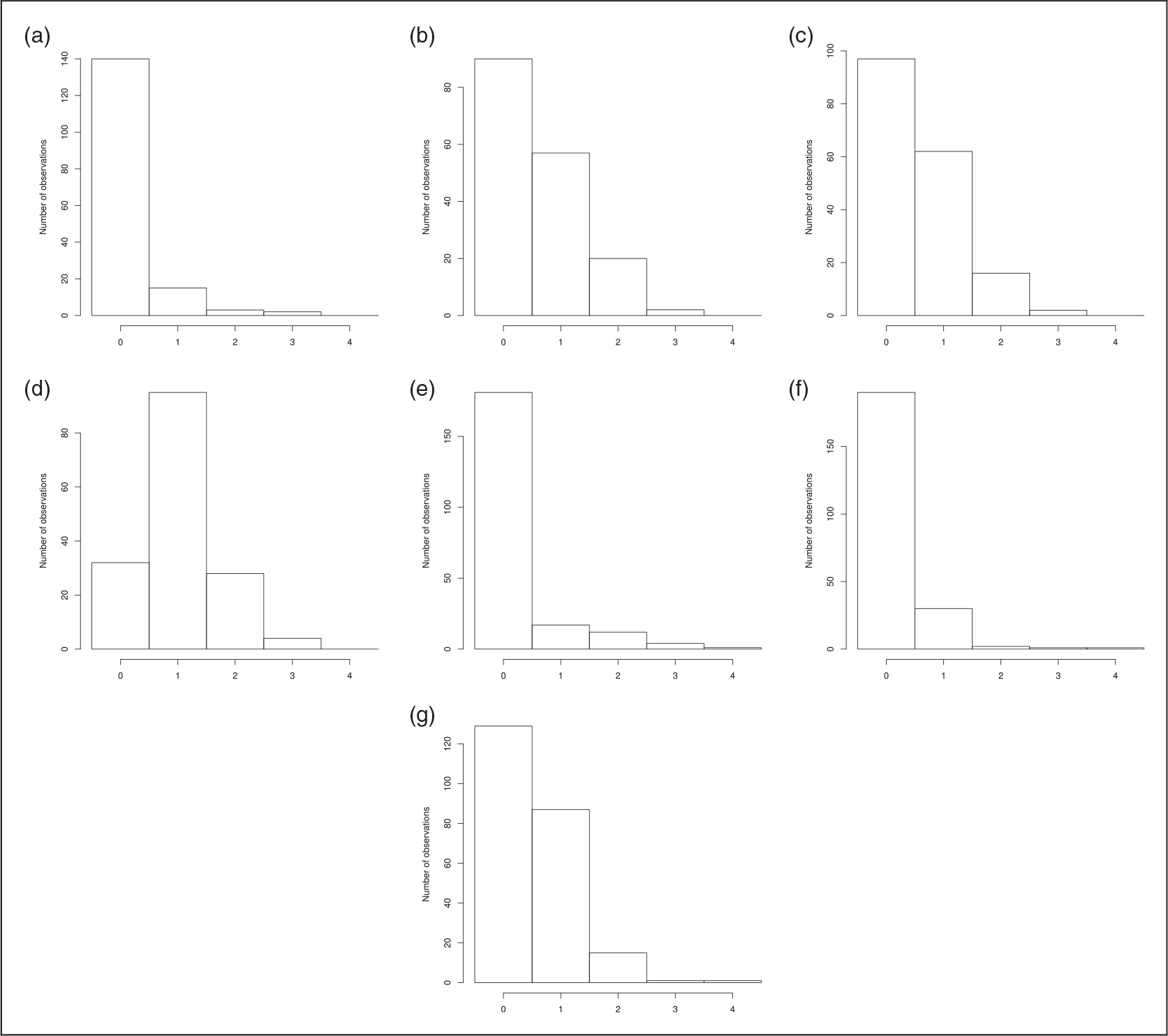
Figure 2.

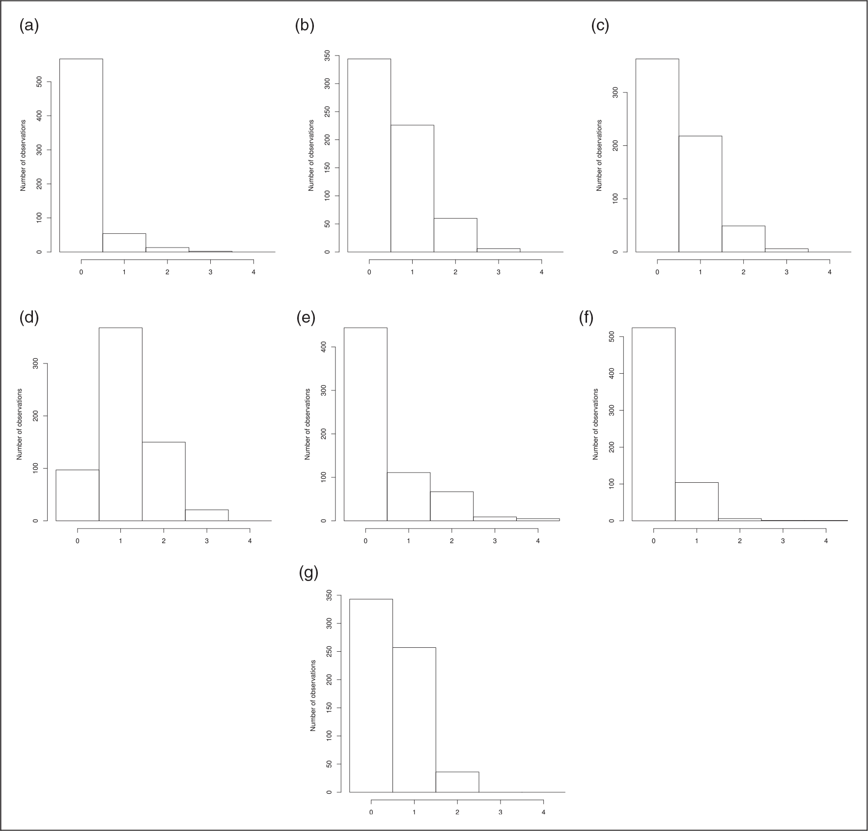
Distribution of toxicities for the n patients with complete observations over all cycles. (a) Vomiting; (b) nausea; (c) diarrhea; (d) asthenia; (e) neutropenia; (f) thrombopenia; and (g) anemia.

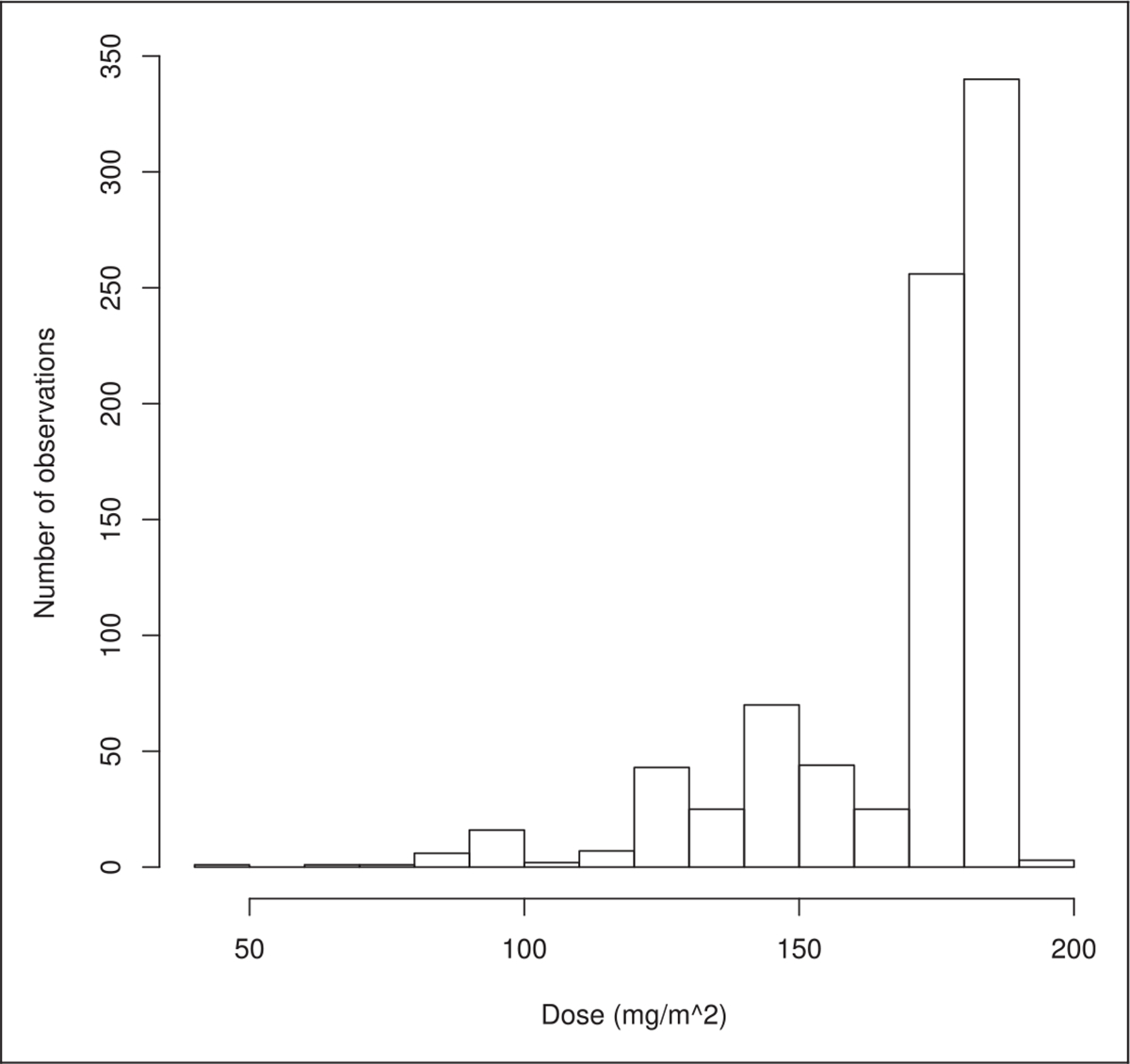
Figure 3.

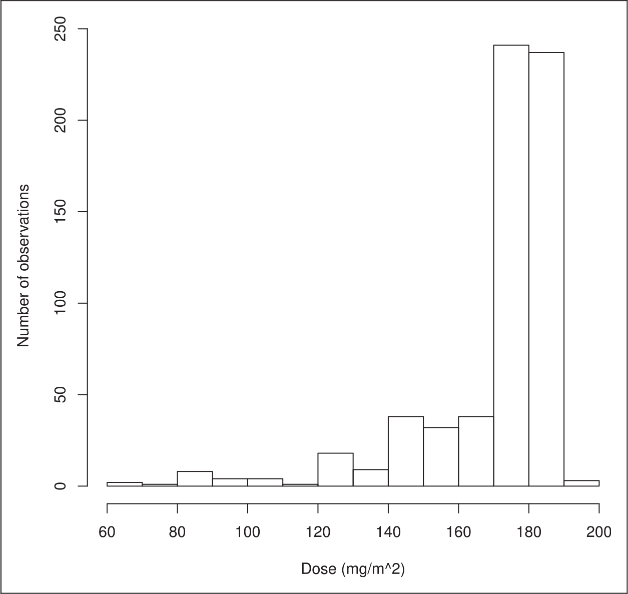
Distribution of doses for the n patients with complete observations over all cycles (sample 1).

Figure 4.

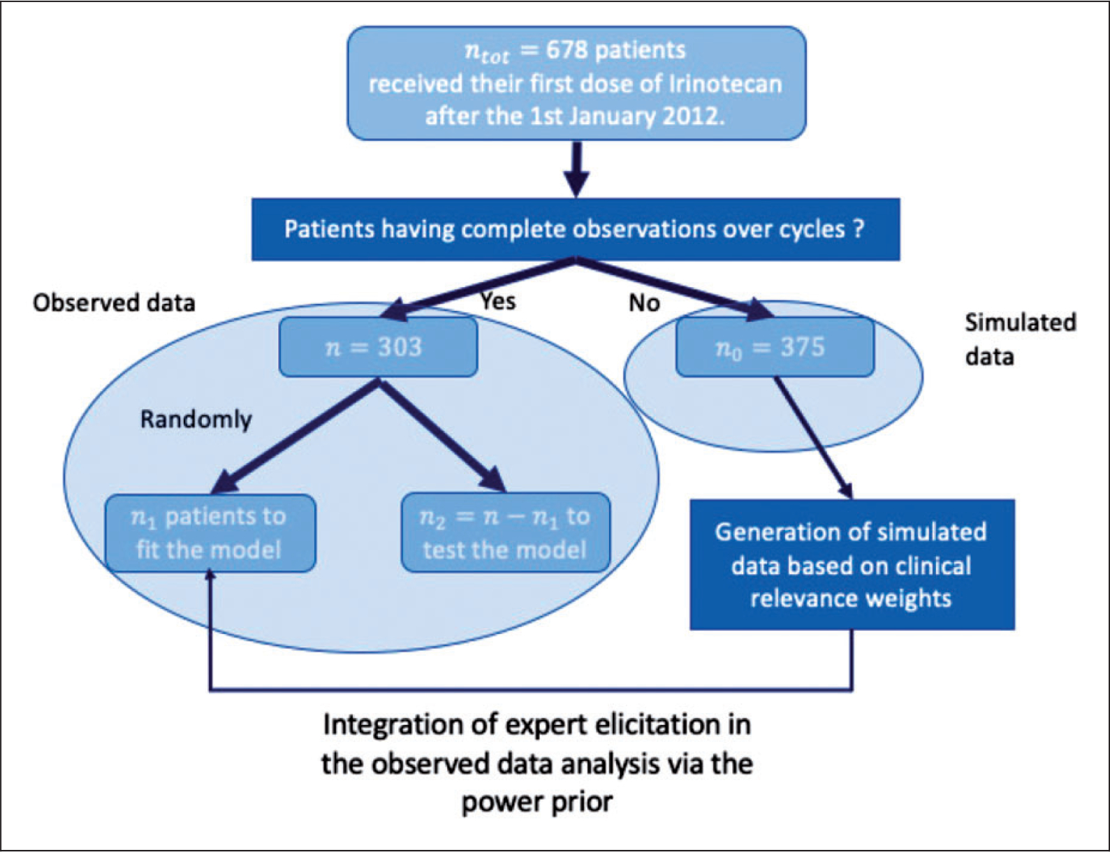
Flowchart of the use of patients.

Figure 5.

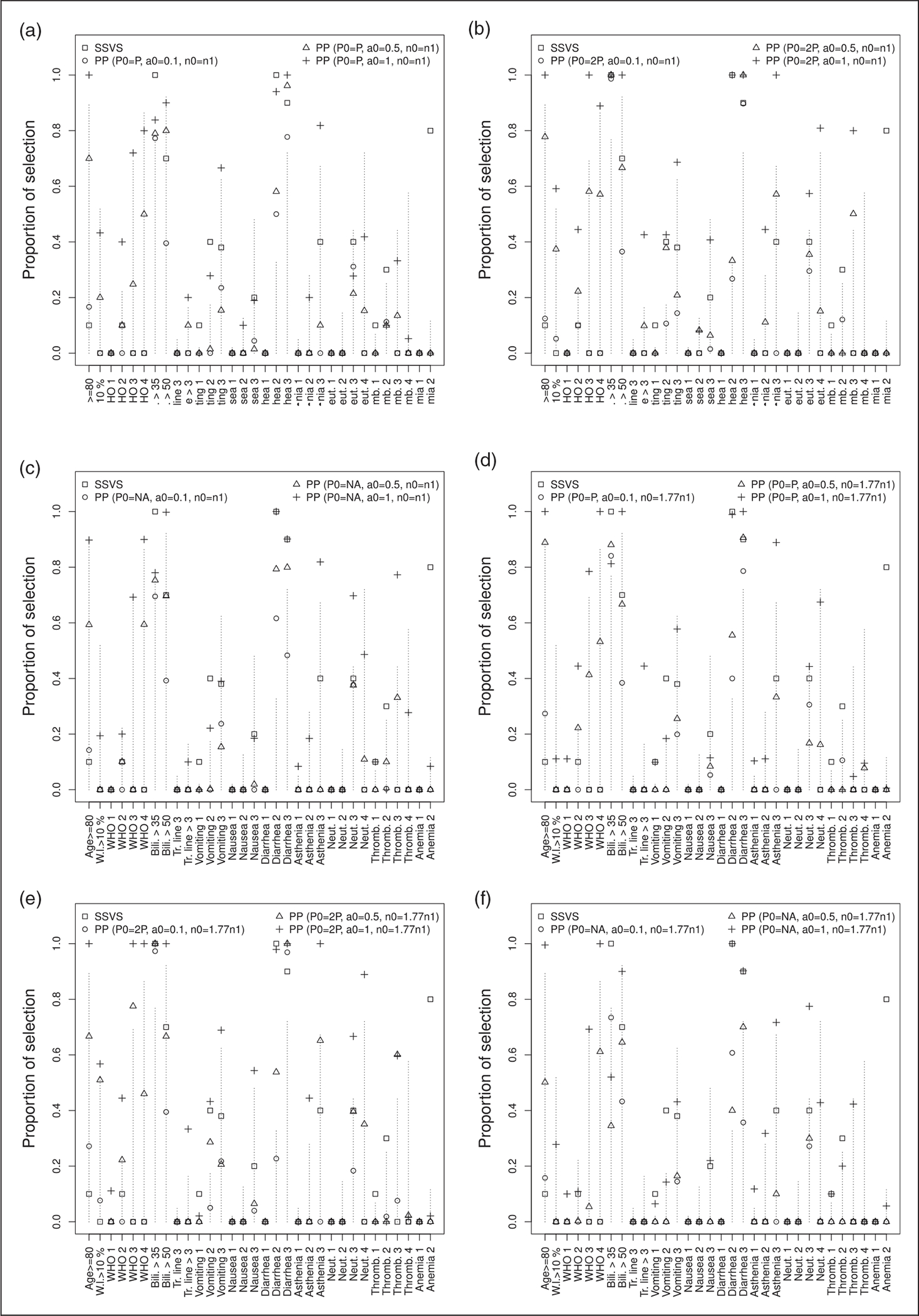
Proportion of times each variable is selected by the models for approach 1, several values of P₀, n₀ and a₀. The values of mean weights elicited by clinicians for each variable are equal to the length of the dashed lines. Each model is labeled with a different symbol. (a) P₀ = P, n₀ = n₁; (b) P₀ = 2P, n₀ = n₁; (c) P₀ = P/2, n₀ = n₁; (d) P₀ = P, n₀ = 1.77 × n₁; (e) P₀ = 2P, n₀ = 1.77 × n₁; and (f) P₀ = P/2, n₀ = 1.77 × n₁.

Figure 6.

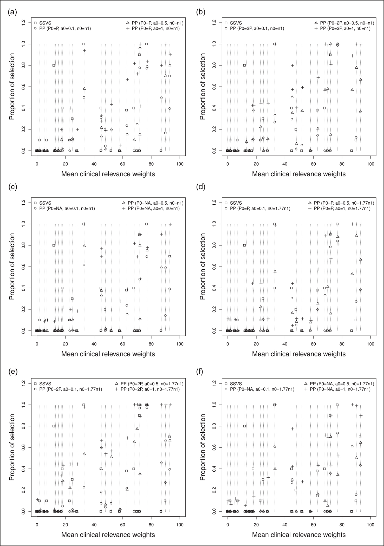
Proportion of times each variable is selected by the models against values of mean weights elicited by clinicians for approach 1, several values of P₀, n₀ and a₀. Each model is labeled with a different symbol. (a) P₀ = P, n₀ = n₁; (b) P₀ = 2P, n₀ = n₁; (c) P₀ = P/2, n₀ = n₁; (d) P₀ = P, n₀ = 1.77 × n₁; (e) P₀ = 2P, n₀ = 1.77 × n₁; and (f) P₀ = P/2, n₀ = 1.77 × n₁.

Figure 7.

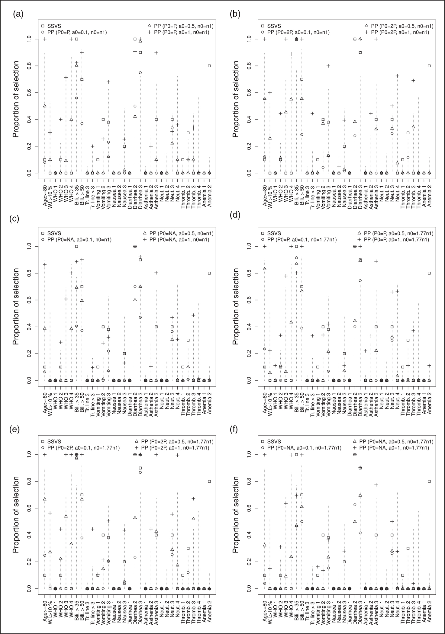
Proportion of times each variable is selected by the models for approach 2, several values of P₀, n₀ and a₀. The values of mean weights elicited by clinicians for each variable are equal to the length of the dashed lines. Each model is labeled with a different symbol. (a) P₀ = P, n₀ = n₁; (b) P₀ = 2P, n₀ = n₁; (c) P₀ = P/2, n₀ = n₁; (d) P₀ = P, n₀ = 1.77 × n₁; (e) P₀ = 2P, n₀ = 1.77 × n₁; and (f) P₀ = P/2, n₀ = 1.77 × n₁.

Figure 8.

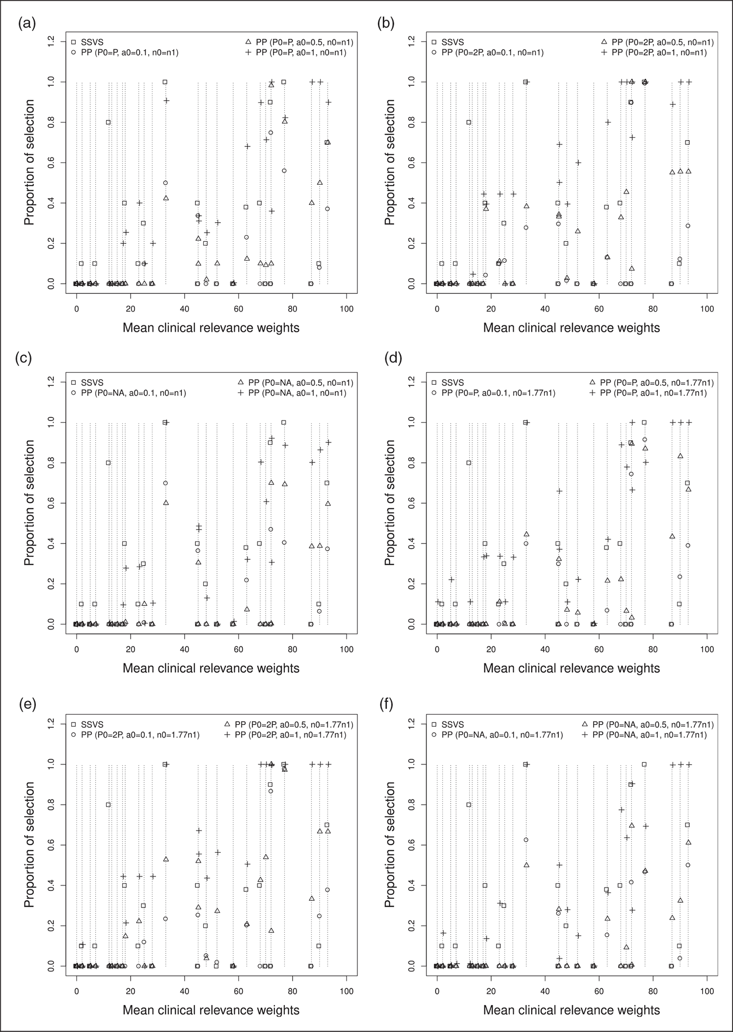
Proportion of times each variable is selected by the models against values of mean weights elicited by clinicians for approach 2, several values of P₀, n₀ and a₀. Each model is labeled with a different symbol. (a) P₀ = P, n₀ = n₁; (b) P₀ = 2P, n₀ = n₁; (c) P₀ = P/2, n₀ = n₁; (d) P₀ = P, n₀ = 1.77 × n₁; (e) P₀ = 2P, n₀ = 1.77 × n₁; and (f) P₀ = P/2, n₀ = 1.77 × n₁.

Table 5.

Estimated coefficients, number of selected variables and AUCs for usual SSVS and SSVS using the power prior for the first approach with P₀ = P, a₀ ∈ {0.1, 0.5, 1}, BMA and several values of n₀.

Variables / Models	*	SSVS	Power prior (P0 = P)
			a0 = 0.1	a0 = 0.5	n0 = n1 a0 = 1	a0 = 0.1	a0 = 0.5	n0 = 1.77 × n1 a0 = 1
Intercept	–	−10.62 (1.36)	−5.17 (0.45)	−6.33 (1.13)	−10.85 (1.55)	−5.05 (0.48)	−6.22 (0.93)	−12.55 (1.9)
Age ≥80 years	5/32	1.630.1 (0.68)	1.590.2 (0.79)	4.160.7 (2.52)	7.951 (3.66)	1.790.3 (1.14)	4.590.9 (2.51)	10.171 (3.21)
Weight loss > 10%	0/5	1.69 (0.64)	0.89 (0.2)	1,290.2 (0.66)	2.780.4 (2.48)	0.84 (0.13)	0.98 (0.16)	1.860.1 (0.74)
ECOG performance status 1	47/381	0.6 (0.23)	0.56 (0.2)	0.69 (0.34)	0.78 (0.29)	0.55 (0.18)	0.67 (0.27)	1.050.1 (0.77)
ECOG performance status 2	25/100	1.870.1 (0.48)	1.08 (0.33)	1.170.1 (0.9)	2.210.4 (1.98)	1.13 (0.38)	1.320.2 (0.81)	3.350.4 (3.08)
ECOG performance status 3	2/11	1.61 (0.38)	1.780.3 (0.56)	2.390.2 (1.87)	5.80.7 (3.11)	0.99 (0.23)	2.860.4 (1.6)	6.980.8 (3.08)
ECOG performance status 4	3/21	1.24 (0.49)	1.450.2 (0.62)	2.90.5 (1.83)	6.570.8 (3.03)	1.06 (0.39)	2.990.5 (1.64)	7.821 (1.36)
Bilirubin >35 μmol/L	1/1	5.941 (0.38)	5.380.8 (0.79)	7.50.8 (3.67)	10.770.8 (4.04)	6.540.8 (1.29)	9.290.9 (2.59)	13.010.8 (5.82)
Bilirubin >50 μmol/L	2/5	4.390.7 (1.64)	2.370.4 (1.17)	4.30.8 (2.52)	8.110.9 (3.59)	2.280.4 (1.2)	4.260.7 (2.59)	9.051 (3.31)
Treatment line 3	8/46	1.28 (0.35)	0.61 (0.2)	0.55 (0.17)	0.7 (0.19)	0.61 (0.23)	0.55 (0.24)	0.76 (0.2)
Treatment line >3	6/43	1.76 (0.6)	0.77 (0.26)	0.950.1 (0.74)	1.840.2 (2.19)	0.77 (0.19)	1.08 (0.52)	3.250.4 (2.84)
Vomiting 1	11/54	1.330.1 (0.52)	0.7 (0.15)	0.78 (0.21)	1.03 (0.25)	0.69 (0.17)	0.83 (0.35)	1.310.1 (0.66)
Vomiting 2	5/13	2.210.4 (0.95)	0.91 (0.3)	0.96 (0.47)	1.430.3 (0.78)	0.87 (0.29)	0.87 (0.5)	1.40.2 (1.17)
Vomiting 3	1/2	3.690.4 (1.86)	2.080.2 (1.81)	2.60.2 (2.96)	4.720.7 (3.1)	2.090.2 (1.84)	2.490.3 (2.54)	5.440.6 (4.91)
Nausea 1	28/226	0.62 (0.13)	0.31 (0.07)	0.3 (0.11)	0.4 (0.15)	0.29 (0.07)	0.29 (0.12)	0.45 (0.13)
Nausea 2	13/60	0.63 (0.12)	0.47 (0.07)	0.5 (0.09)	0.730.1 (0.53)	0.45 (0.08)	0.44 (0.13)	0.53 (0.15)
Nausea 3	2/6	2.210.2 (2.27)	0.95 (0.51)	1.08 (0.45)	2.280.2 (2.34)	0.940.1 (0.52)	1.140.1 (1)	2.130.1 (3)
Diarrhea 1	28/218	0.48 (0.11)	0.29 (0.1)	0.29 (0.13)	0.37 (0.14)	0.28 (0.09)	0.26 (0.11)	0.33 (0.09)
Diarrhea 2	18/49	6.541 (1.88)	2.160.5 (0.61)	2.470.6 (0.99)	4.310.9 (1.21)	2.030.4 (0.6)	2.310.6 (0.78)	5.21 (1.27)
Diarrhea 3	4/6	6.490.9 (2.48)	3.640.8 (1.22)	5.891 (2.76)	9.461 (2.97)	3.420.8 (1.23)	5.70.9 (2.47)	10.841 (4.28)
Asthenia 1	41/368	0.66 (0.17)	0.5 (0.11)	0.62 (0.17)	0.88 (0.23)	0.51 (0.12)	0.67 (0.23)	1.090.1 (0.64)
Asthenia 2	32/150	0.83 (0.18)	0.7 (0.21)	0.87 (0.36)	1.650.2 (1.15)	0.72 (0.25)	0.86 (0.49)	1.780.1 (1.85)
Asthenia 3	4/21	2.260.4 (0.8)	1.02 (0.2)	1.550.1 (0.53)	3.920.8 (1.75)	1.04 (0.2)	1.940.3 (0.77)	5.980.9 (2.77)
Neutropenia 1	12/111	0.65 (0.15)	0.39 (0.09)	0.4 (0.14)	0.51 (0.18)	0.37 (0.08)	0.38 (0.11)	0.54 (0.19)
Neutropenia 2	9/67	0.65 (0.05)	0.46 (0.07)	0.48 (0.1)	0.63 (0.14)	0.44 (0.07)	0.41 (0.08)	0.54 (0.11)
Neutropenia 3	4/9	3.730.4 (2.12)	1.680.3 (0.83)	1.810.2 (1.16)	2.930.3 (2.89)	1.690.3 (0.85)	1.550.2 (0.71)	2.710.4 (1.48)
Neutropenia 4	1/5	1.81 (0.48)	1.05 (0.24)	1.550.2 (1.09)	3.230.4 (1.85)	1.09 (0.23)	1.850.2 (1.25)	4.710.7 (2.8)
Thrombopenia 1	15/104	1.490.1 (0.61)	0.52 (0.13)	0.55 (0.15)	0.96 (0.35)	0.49 (0.1)	0.5 (0.13)	1.07 (0.37)
Thrombopenia 2	2/6	3.220.3 (1.35)	1.050.1 (0.7)	0.710.1 (0.53)	1.10.1 (1.6)	0.960.1 (0.61)	0.48 (0.12)	0.57 (0.14)
Thrombopenia 3	0/1	3.21 (0.52)	1.36 (0.17)	1.550.1 (0.67)	2.990.3 (2.73)	1.29 (0.17)	1.17 (0.27)	1.81 (0.61)
Thrombopenia 4	0/1	1.13 (0.11)	0.89 (0.04)	0.9 (0.11)	1.030.1 (0.31)	0.91 (0.05)	1.090.1 (0.4)	1.630.1 (1.21)
Anemia 1	26/257	0.42 (0.09)	0.19 (0.04)	0.19 (0.05)	0.26 (0.07)	0.18 (0.03)	0.18 (0.03)	0.3 (0.07)
Anemia 2	12/36	3.250.8 (1.09)	1.18 (0.26)	0.9 (0.19)	1.08 (0.35)	1.16 (0.24)	0.86 (0.23)	1.03 (0.32)
Number of selected variables	–	5	3	6	9	2	6	10
AUC	–	0.69 (0.04)	0.68 (0.03)	0.68 (0.04)	0.68 (0.05)	0.68 (0.03)	0.68 (0.04)	0.68 (0.04)

Note: ^s, 0 ≤ s ≤ 1 is the proportion of times a variable is selected by the model. The * column indicates the proportion of dose reductions linked to the variable.

Table 6.

Estimated coefficients, number of selected variables and AUCs for usual SSVS and SSVS using the power prior for the first approach with P₀ = 2P, a₀ ∈ {0.1, 0.5, 1}, BMA and several values of n₀.

Variables/Models	*	SSVS	Power prior (P0 = 2P)
			a0 = 0.1	a0 = 0.5	n0 = n0 a0 = 1	a0 = 0.1	a0 = 0.5	n0 = 1.77 × n1 a0 = 1
Intercept	–	−10.62 (1.36)	−4.59 (0.33)	−5.64 (0.78)	−11.45 (2.7)	−4.43 (0.39)	−5.61 (0.93)	−11.72 (2)
Age ≥80 years	5/32	1.630.1 (0.68)	1.340.1 (0.47)	4.050.8 (1.9)	9.711 (2.66)	1.430.3 (0.74)	4.270.7 (2.17)	10.371 (2.31)
Weight loss > 10%	0/5	1.69 (0.64)	1.260.1 (0.44)	2.350.4 (1.35)	4.930.6 (2.83)	1.260.1 (0.56)	2.910.5 (2.22)	5.560.6 (3.48)
ECOG performance status 1	47/381	0.6 (0.23)	0.51 (0.19)	0.54 (0.24)	0.64 (0.24)	0.5 (0.19)	0.54 (0.24)	0.760.1 (0.57)
ECOG performance status 2	25/100	1.870.1 (0.48)	1.270.1 (0.47)	1.390.2 (1.13)	3.110.4 (3.41)	1.28 (0.48)	1.380.2 (0.97)	3.380.4 (3.33)
ECOG performance status 3	2/11	1.61 (0.38)	1.07 (0.33)	3.150.6 (1.56)	8.551 (2.59)	1.11 (0.23)	3.520.8 (1.78)	9.591 (2.71)
ECOG performance status 4	3/21	1.24 (0.49)	0.96 (0.19)	2.470.6 (1.14)	6.540.9 (2.61)	0.98 (0.22)	2.390.5 (1.09)	7.061 (2.1)
Bilirubin >35 μmol/L	l/l	5.941 (0.38)	6.821 (0.83)	9.391 (2.92)	13.041 (2.56)	6.491 (0.84)	9.651 (2.88)	14.551 (2.07)
Bilirubin >50 μmol/L	2/5	4.390.7 (1.64)	2.150.4 (0.99)	4.130.7 (2.33)	9.581 (3.22)	20.4 (0.95)	4.360.7 (2.51)	9.951 (3.64)
Treatment line 3	8/46	1.28 (0.35)	0.56 (0.19)	0.52 (0.2)	0.62 (0.16)	0.51 (0.21)	0.47 (0.22)	0.61 (0.18)
Treatment line >3	6/43	1.76 (0.6)	0.71 (0.18)	1.080.1 (0.65)	3.180.4 (3.08)	0.65 (0.13)	0.8 (0.37)	2.30.3 (2.42)
Vomiting 1	11/54	1.330.1 (0.52)	0.62 (0.16)	0.71 (0.25)	1.05 (0.31)	0.6 (0.17)	0.7 (0.33)	1.09 (0.53)
Vomiting 2	5/13	2.210.4 (0.95)	1.220.1 (0.67)	2.30.4 (2)	4.530.4 (4.42)	1.030.1 (0.37)	1.540.3 (1.46)	3.590.4 (3.72)
Vomiting 3	1/2	3.690.4 (1.86)	2.030.1 (1.62)	2.980.2 (2.5)	6.420.7 (3.33)	2.10.2 (1.72)	2.620.2 (2.26)	6.920.7 (4.18)
Nausea 1	28/226	0.62 (0.13)	0.29 (0.06)	0.28 (0.1)	0.39 (0.11)	0.26 (0.07)	0.27 (0.13)	0.38 (0.13)
Nausea 2	13/60	0.63 (0.12)	0.42 (0.06)	0.530.1 (0.44)	1.080.1 (1.44)	0.39 (0.06)	0.34 (0.1)	0.47 (0.19)
Nausea 3	2/6	2.210.2 (2.27)	0.89 (0.41)	1.270.1 (1.09)	2.980.4 (2.5)	0.9 (0.39)	1.360.1 (1.29)	3.240.5 (3.15)
Diarrhea 1	28/218	0.48 (0.11)	0.31 (0.09)	0.32 (0.13)	0.41 (0.13)	0.29 (0.09)	0.29 (0.13)	0.37 (0.15)
Diarrhea 2	18/49	6.541 (1.88)	1.790.2 (0.56)	2.350.3 (1.31)	5.451 (2.16)	1.790.2 (0.48)	2.820.5 (1.57)	6.371 (1.33)
Diarrhea 3	4/6	6.490.9 (2.48)	4.310.9 (1.37)	7.671 (2.51)	15.081 (3.69)	4.281 (1.43)	7.831 (3.14)	15.281 (3.93)
Asthenia 1	41/368	0.66 (0.17)	0.39 (0.07)	0.49 (0.15)	0.84 (0.39)	0.4 (0.1)	0.53 (0.21)	1.04 (0.54)
Asthenia 2	32/150	0.83 (0.18)	0.66 (0.23)	1.170.1 (0.79)	3.10.4 (2.81)	0.63 (0.21)	1.12 (0.69)	3.220.4 (2.65)
Asthenia 3	4/21	2.260.4 (0.8)	0.98 (0.21)	2.570.6 (1.27)	7.641 (2.02)	1.05 (0.29)	2.960.7 (1.48)	8.391 (1.63)
Neutropenia 1	12/111	0.65 (0.15)	0.34 (0.07)	0.35 (0.09)	0.55 (0.15)	0.33 (0.05)	0.3 (0.04)	0.46 (0.1)
Neutropenia 2	9/67	0.65 (0.05)	0.42 (0.07)	0.41 (0.09)	0.52 (0.13)	0.39 (0.07)	0.33 (0.05)	0.43 (0.07)
Neutropenia 3	4/9	3.730.4 (2.12)	1.770.3 (0.96)	2.580.4 (1.79)	4.920.6 (3.64)	1.530.2 (0.69)	2.980.4 (2.13)	5.420.7 (4.09)
Neutropenia 4	1/5	1.81 (0.48)	1.05 (0.26)	1.950.2 (1.06)	5.940.8 (2.54)	1.13 (0.34)	2.930.4 (2.22)	7.410.9 (3.51)
Thrombopenia 1	15/104	1.490.1 (0.61)	0.41 (0.08)	0.4 (0.08)	0.78 (0.21)	0.38 (0.09)	0.38 (0.11)	0.8 (0.28)
Thrombopenia 2	2/6	3.220.3 (1.35)	1.380.1 (1.26)	0.62 (0.17)	0.69 (0.24)	0.89 (0.17)	0.52 (0.11)	0.61 (0.2)
Thrombopenia 3	0/1	3.21 (0.52)	1.51 (0.26)	4.040.5 (3.02)	8.510.8 (5.67)	1.480.1 (0.29)	3.820.6 (2.57)	6.750.6 (4.93)
Thrombopenia 4	0/1	1.13 (0.11)	0.91 (0.06)	1 (0.25)	1.39 (0.55)	0.93 (0.06)	1.07 (0.19)	1.27 (0.46)
Anemia 1	26/257	0.42 (0.09)	0.17 (0.03)	0.17 (0.05)	0.28 (0.09)	0.16 (0.02)	0.16 (0.03)	0.27 (0.05)
Anemia 2	12/36	3.250.8 (1.09)	1.12 (0.27)	0.83 (0.22)	1.02 (0.29)	1.04 (0.21)	0.82 (0.22)	0.97 (0.31)
Number of selected variables	–	5	2	8	13	2	10	14
AUC	–	0.69 (0.04)	0.69 (0.03)	0.68 (0.04)	0.68 (0.04)	0.69 (0.04)	0.69 (0.05)	0.69 (0.05)

Note: ^s, 0 ≤ s ≤ 1 is the proportion of times a variable is selected by the model. The * column indicates the proportion of dose reductions linked to the variable.

Table 7.

Estimated coefficients, number of selected variables and AUCs for usual SSVS and SSVS using the power prior for the first approach with P₀ = P/2, a₀ ∈ {0.1, 0.5, 1}, BMA and several values of n₀.

Variables / Models	*	SSVS	Power prior (P0 = P/2)
			a0 = 0.1	a0 = 0.5	n0 = n0 a0 = 1	a0 = 0.1	a0 = 0.5	n0 = 1.77 × n1 a0 = 1
Intercept	–	−10.62 (1.36)	−5.39 (0.41)	−6.54 (0.9)	−12.14 (2)	−5.32 (0.42)	−6.16 (1.3)	−12.11 (1.77)
Age ≥80 years	5/32	1.630.1 (0.68)	1.450.1 (0.66)	4.160.6 (2.91)	7.740.9 (4.51)	1,540.2 (0.75)	4.140.5 (3.46)	8.921 (5.08)
Weight loss > 10%	0/5	1.69 (0.64)	0.82 (0.16)	0.9 (0.27)	2.030.2 (1.29)	0.86 (0.19)	1.11 (0.42)	2.160.3 (1.49)
ECOG performance status 1	47/381	0.6 (0.23)	0.56 (0.18)	0.7 (0.25)	0.84 (0.38)	0.54 (0.17)	0.57 (0.22)	0.820.1 (0.68)
ECOG performance status 2	25/100	1.870.1 (0.48)	1 (0.27)	0.960.1 (0.69)	1.770.2 (2.35)	0.92 (0.2)	0.57 (0.17)	1.180.1 (1.44)
ECOG performance status 3	2/11	1.61 (0.38)	1.780.3 (0.56)	1.2 (0.42)	3.560.7 (1.21)	0.88 (0.12)	1.150.1 (0.39)	3.490.7 (1.85)
ECOG performance status 4	3/21	1.24 (0.49)	1,450.2 (0.62)	3.280.6 (1.93)	8.050.9 (3.84)	1.07 (0.27)	3.10.6 (1.64)	8.081 (2.23)
Bilirubin > 35 μmol/L	l/l	5.941 (0.38)	4.790.7 (1.79)	7.220.8 (4.72)	9.511 (5.4)	5.910.7 (0.99)	5.060.3 (5.6)	9.150.5 (7.34)
Bilirubin > 50 μmol/L	2/5	4.390.7 (1.64)	2.410.4 (1.04)	4.540.7 (2.59)	9.551 (4.15)	2.350.4 (0.97)	4.330.6 (2.84)	8.760.9 (4.53)
Treatment line 3	8/46	1.28 (0.35)	0.65 (0.2)	0.61 (0.2)	0.77 (0.19)	0.64 (0.21)	0.58 (0.29)	0.79 (0.34)
Treatment line >3	6/43	1.76 (0.6)	0.72 (0.16)	0.75 (0.24)	1.120.1 (0.63)	0.68 (0.14)	0.62 (0.15)	0.87 (0.15)
Vomiting 1	11/54	1.330.1 (0.52)	0.73 (0.15)	0.83 (0.23)	1.25 (0.44)	0.74 (0.16)	0.87 (0.21)	1.550.1 (0.39)
Vomiting 2	5/13	2.210.4 (0.95)	0.9 (0.26)	0.89 (0.41)	1.780.2 (1.56)	0.84 (0.24)	0.74 (0.31)	1.190.1 (1.02)
Vomiting 3	1/2	3.690.4 (1.86)	1.990.2 (1.47)	1.950.2 (1.48)	4.210.4 (3.35)	1.930.1 (1.33)	1.970.2 (1.38)	4.490.4 (3.15)
Nausea 1	28/226	0.62 (0.13)	0.32 (0.06)	0.31 (0.09)	0.46 (0.11)	0.3 (0.06)	0.29 (0.1)	0.44 (0.12)
Nausea 2	13/60	0.63 (0.12)	0.48 (0.07)	0.5 (0.06)	0.71 (0.25)	0.48 (0.07)	0.52 (0.05)	0.7 (0.17)
Nausea 3	2/6	2.210.2 (2.27)	0.93 (0.4)	0.97 (0.31)	1.930.2 (2.02)	0.89 (0.38)	0.92 (0.3)	1.70.2 (1.32)
Diarrhea 1	28/218	0.48 (0.11)	0.29 (0.09)	0.27 (0.12)	0.34 (0.1)	0.28 (0.08)	0.26 (0.1)	0.34 (0.09)
Diarrhea 2	18/49	6.541 (1.88)	2.320.6 (0.58)	2.780.8 (0.91)	5.611 (1.14)	2.260.6 (0.59)	2.50.4 (1.09)	5.441 (1.2)
Diarrhea 3	4/6	6.490.9 (2.48)	2.330.5 (0.89)	3.150.8 (1.39)	70.9 (3.28)	2.330.4 (0.82)	2.440.4 (0.82)	6.080.9 (2.7)
Asthenia 1	41/368	0.66 (0.17)	0.52 (0.11)	0.63 (0.14)	1.010.7 (0.7)	0.54 (0.12)	0.66 (0.18)	1.050.1 (0.54)
Asthenia 2	32/150	0.83 (0.18)	0.75 (0.19)	0.84 (0.34)	1.310.2 (0.88)	0.78 (0.21)	1 (0.35)	1.740.3 (1.3)
Asthenia 3	4/21	2.260.4 (0.8)	1.03 (0.19)	1.4 (0.32)	3.730.8 (1.48)	1.02 (0.15)	1.480.1 (0.35)	4.40.7 (1.96)
Neutropenia 1	12/111	0.65 (0.15)	0.41 (0.1)	0.43 (0.13)	0.62 (0.16)	0.4 (0.09)	0.37 (0.11)	0.56 (0.15)
Neutropenia 2	9/67	0.65 (0.05)	0.47 (0.08)	0.51 (0.13)	0.65 (0.18)	0.44 (0.07)	0.43 (0.07)	0.57 (0.1)
Neutropenia 3	4/9	3.730.4 (2.12)	1.840.4 (0.84)	2.220.4 (1.2)	3.470.7 (1.92)	1.740.3 (0.67)	2.180.3 (1.03)	4.160.8 (1.64)
Neutropenia 4	1/5	1.81 (0.48)	1.07 (0.23)	1.370.1 (0.64)	2.640.5 (1.64)	1.04 (0.18)	1.31 (0.42)	2.780.4 (1.22)
Thrombopenia 1	15/104	1.490.1 (0.61)	0.58 (0.14)	0.63 (0.15)	1.240.1 (0.55)	0.57 (0.15)	0.58 (0.15)	1.40.1 (0.78)
Thrombopenia 2	2/6	3.220.3 (1.35)	0.88 (0.25)	0.740.1 (0.55)	0.69 (0.29)	0.82 (0.2)	0.8 (0.41)	1.410.2 (1.39)
Thrombopenia 3	0/1	3.21 (0.52)	1.45 (0.12)	2.270.3 (0.88)	4.790.8 (1.97)	1.34 (0.11)	1.52 (0.14)	4.070.4 (2.38)
Thrombopenia 4	0/1	1.13 (0.11)	0.92 (0.05)	1.08 (0.34)	1.580.3 (1.14)	0.9 (0.04)	1.14 (0.3)	0.95 (0.17)
Anemia 1	26/257	0.42 (0.09)	0.2 (0.04)	0.2 (0.06)	0.31 (0.11)	0.19 (0.03)	0.18 (0.05)	0.28 (0.09)
Anemia 2	12/36	3.250.8 (1.09)	1.24 (0.25)	1.03 (0.22)	1.250.1 (0.46)	1.21 (0.21)	1.02 (0.12)	1.350.1 (0.33)
Number of selected variables	–	5	3	6	11	2	4	9
AUC	–	0.69 (0.04)	0.69 (0.03)	0.69 (0.04)	0.68 (0.04)	0.68 (0.03)	0.68 (0.04)	0.68 (0.03)

Note: ^s, 0 ≤ s ≤ 1 is the proportion of times a variable is selected by the model. The * column indicates the proportion of dose reductions linked to the variable.

Table 8.

Estimated coefficients, number of selected variables and AUCs for usual SSVS and SSVS using the power prior for the second approach with P₀ = P, a₀ ∈ {0.1, 0.5, 1}, BMA and several values of n₀.

Variables / Models	*	SSVS	Power prior (P0 = P)
			a0 = 0.1	a0 = 0.5	n0 = n1 a0 = 1	a0 = 0.1	a0 = 0.5	n0 = 1.77 × n1 a0 = 1
Intercept	–	−10.62 (1.36)	−5.27 (0.48)	−5.61 (0.51)	−10.3 (1.76)	−5.05 (0.51)	−5.79 (0.93)	−11.65 (1.29)
Age ≥80 years	5/32	1.630.1 (0.68)	1.40.1 (0.7)	2.990.5 (1.65)	6.141 (2.63)	1.690.2 (0.94)	3.930.8 (2.13)	8.861 (4.47)
Weight loss > 10%	0/5	1.69 (0.64)	0.87 (0.18)	1.060.1 (0.57)	2.170.3 (2.19)	0.83 (0.12)	10.4 (0.4)	2.190.2 (2.02)
ECOG performance status 1	47/381	0.6 (0.23)	0.56 (0.19)	0.62 (0.19)	0.81 (0.29)	0.55 (0.19)	0.61 (0.24)	0.940.1 (0.59)
ECOG performance status 2	25/100	1.870.1 (0.48)	1.04 (0.27)	0.89 (0.52)	1.840.4 (1.71)	1.1 (0.37)	1.070.1 (0.71)	2.160.3 (2.3)
ECOG performance status 3	2/11	1.61 (0.38)	0.91 (0.17)	1.420,1 (0.59)	4.120.7 (2.01)	0.92 (0.18)	1.530.1 (0.57)	4.70.8 (2.17)
ECOG performance status 4	3/21	1.24 (0.49)	1.05 (0.29)	2.340.4 (1.31)	6.051 (2.11)	1.02 (0.31)	2.520.4 (1.23)	7.451 (1.58)
Bilirubin >35 μmol/L	l/l	5.941 (0.38)	4.370.6 (1.75)	5.150.8 (3.04)	8.350.8 (4.18)	6.970.9 (1.14)	9.130.9 (2.84)	13.090.8 (6.47)
Bilirubin >50 μmol/L	2/5	4.390.7 (1.64)	2.360.4 (1.07)	3.460.7 (1.73)	7.410.9 (3.1)	2.220.4 (1.06)	3.750.7 (2.18)	8.441 (3.68)
Treatment line 3	8/46	1.28 (0.35)	0.62 (0.19)	0.52 (0.16)	0.63 (0.14)	0.59 (0.21)	0.51 (0.2)	0.77 (0.21)
Treatment line >3	6/43	1.76 (0.6)	0.76 (0.22)	0.79 (0.42)	1.580.2 (1.45)	0.77 (0.18)	0.96 (0.5)	2.360.3 (2.35)
Vomiting 1	11/54	1.330.1 (0.52)	0.7 (0.14)	0.7 (0.19)	0.99 (0.26)	0.69 (0.16)	0.76 (0.21)	1.21 (0.34)
Vomiting 2	5/13	2.210.4 (0.95)	0.92 (0.3)	0.91 (0.47)	1.530.3 (0.98)	0.84 (0.26)	0.88 (0.48)	1.810.3 (1.53)
Vomiting 3	1/2	3.690.4 (1.86)	2.120.2 (1.78)	2.250.1 (2.39)	4.90.7 (3.09)	1.660.1 (1.06)	2.320.2 (2.55)	5.050.4 (5.04)
Nausea 1	28/226	0.62 (0.13)	0.31 (0.06)	0.24 (0.05)	0.33 (0.09)	0.29 (0.06)	0.26 (0.09)	0.41 (0.12)
Nausea 2	13/60	0.63 (0.12)	0.47 (0.08)	0.5 (0.11)	0.74 (0.46)	0.46 (0.08)	0.47 (0.14)	0.61 (0.19)
Nausea 3	2/6	2.210.2 (2.27)	0.93 (0.4)	1 (0.34)	2.550.3 (2.31)	0.87 (0.32)	10.1 (0.65)	1.870.1 (2.26)
Diarrhea 1	28/218	0.48 (0.11)	0.3 (0.09)	0.26 (0.1)	0.35 (0.11)	0.27 (0.08)	0.23 (0.09)	0.29 (0.1)
Diarrhea 2	18/49	6.541 (1.88)	2.220.5 (0.63)	2.090.4 (0.62)	4.070.9 (1.32)	2.050.4 (0.57)	2.180.4 (0.69)	4.951 (0.93)
Diarrhea 3	4/6	6.490.9 (2.48)	3.20.7 (1.03)	4.071 (0.93)	7.921 (1.64)	3.120.7 (1.1)	4.170.9 (1.46)	8.221 (3.01)
Asthenia 1	41/368	0.66 (0.17)	0.52 (0.11)	0.61 (0.12)	0.93 (0.25)	0.51 (0.12)	0.71 (0.25)	1.350.2 (0.88)
Asthenia 2	32/150	0.83 (0.18)	0.75 (0.21)	0.89 (0.31)	1.680.2 (1.03)	0.71 (0.21)	0.83 (0.35)	1.830.3 (1.48)
Asthenia 3	4/21	2.260.4 (0.8)	1.09 (0.23)	1.520.1 (0.48)	4.150.9 (1.71)	1.04 (0.23)	1.710.2 (0.57)	5.150.9 (1.75)
Neutropenia 1	12/111	0.65 (0.15)	0.39 (0.09)	0.37 (0.12)	0.5 (0.16)	0.37 (0.08)	0.37 (0.08)	0.55 (0.16)
Neutropenia 2	9/67	0.65 (0.05)	0.46 (0.08)	0.43 (0.1)	0.56 (0.17)	0.44 (0.07)	0.4 (0.08)	0.57 (0.31)
Neutropenia 3	4/9	3.730.4 (2.12)	1.750.3 (0.91)	1.780.2 (1.21)	2.910.3 (2.97)	1.640.3 (0.74)	1.660.3 (0.74)	3.520.7 (1.8)
Neutropenia 4	1/5	1.81 (0.48)	1.06 (0.23)	1.40.1 (0.92)	2.730.4 (2.17)	1.04 (0.18)	1.31 (0.37)	3.230.7 (1.62)
Thrombopenia 1	15/104	1.490.1 (0.61)	0.54 (0.14)	0.5 (0.13)	0.95 (0.42)	0.5 (0.11)	0.47 (0.14)	0.97 (0.31)
Thrombopenia 2	2/6	3.220.3 (1.35)	1.060.1 (0.73)	0.65 (0.49)	10.4 (1.41)	0.9 (0.46)	0.53 (0.21)	10.1 (1.28)
Thrombopenia 3	0/1	3.21 (0.52)	1.42 (0.17)	1.50.1 (0.65)	2.870.3 (2.71)	1.27 (0.11)	1.3 (0.23)	3.580.4 (3.16)
Thrombopenia 4	0/1	1.13 (0.11)	0.89 (0.05)	0.87 (0.08)	0.92 (0.05)	0.91 (0.04)	0.93 (0.11)	1.02 (0.2)
Anemia 1	26/257	0.42 (0.09)	0.2 (0.04)	0.17 (0.04)	0.26 (0.09)	0.18 (0.03)	0.17 (0.03)	0.26 (0.08)
Anemia 2	12/36	3.250.8 (1.09)	1.21 (0.26)	0.9 (0.18)	1.14 (0.43)	1.17 (0.23)	0.86 (0.16)	1.280.1 (0.8)
Number of selected variables	–	5	3	4	9	2	4	10
AUC	–	0.69 (0.04)	0.68 (0.03)	0.68 (0.04)	0.69 (0.05)	0.6 (0.03)	0.68 (0.05)	0.68 (0.05)

Note: ^s, 0 ≤ s ≤ 1 is the proportion of times a variable is selected by the model. The * column indicates the proportion of dose reductions linked to the variable.

Table 9.

Estimated coefficients, number of selected variables and AUCs for usual SSVS and SSVS using the power prior for the second approach with P₀ = 2P, a₀ ∈ {0.1, 0.5, 1}, BMA and several values of n₀.

Variables / Models	*	SSVS	Power prior (P0 = 2P)
			a0 = 0.1	a0 = 0.5	n0 = n0 a0 = 1	a0 = 0.1	a0 = 0.5	n0 = 1.77 × n1 a0 = 1
Intercept	–	−10.62 (1.36)	−4.66 (0.37)	−5.36 (0.7)	−11.15 (2.29)	−4.5 (0.39)	−5.28 (0.72)	−11.43 (1.84)
Age ≥80 years	5/32	1.630.1 (0.68)	1.330.1 (0.52)	3.570.6 (1.95)	8.821 (2.64)	1.460.2 (0.81)	3.770.7 (2.01)	9.851 (2.74)
Weight loss > 10%	0/5	1.69 (0.64)	1.1 (0.41)	1.690.3 (0.88)	3.870.6 (2.83)	1.04 (0.28)	1.680.3 (0.66)	3.780.6 (2.11)
ECOG performance status 1	47/381	0.6 (0.23)	0.52 (0.19)	0.54 (0.2)	0.68 (0.2)	0.5 (0.17)	0.54 (0.21)	0.75 (0.45)
ECOG performance status 2	25/100	1.870.1 (0.48)	1.230.1 (0.43)	1.230.1 (0.89)	2.990.4 (3.04)	1.22 (0.4)	1,320.2 (0.89)	3.290.4 (3.11)
ECOG performance status 3	2/11	1.61 (0.38)	1.01 (0.23)	2.580.5 (1.12)	7.711 (1.5)	0.99 (0.22)	2.840.5 (1.65)	8.71 (2.02)
ECOG performance status 4	3/21	1.24 (0.49)	0.96 (0.2)	2.240.6 (0.87)	6.530.9 (2.25)	0.95 (0.26)	2.210.3 (0.96)	7.131 (1.49)
Bilirubin >35 μmol/L	l/l	5.941 (0.38)	6.291 (0.79)	6.961 (2.43)	10.221 (1.07)	6.291 (1.05)	8.661 (2.11)	13.461 (1.79)
Bilirubin >50 μmol/L	2/5	4.390.7 (1.64)	2.140.3 (0.99)	3.610.6 (2.33)	8.641 (2.89)	2.020.4 (0.97)	3.810.7 (2.08)	9.551 (3.13)
Treatment line 3	8/46	1.28 (0.35)	0.56 (0.2)	0.49 (0.21)	0.6 (0.18)	0.53 (0.22)	0.44 (0.21)	0.55 (0.21)
Treatment line >3	6/43	1.76 (0.6)	0.74 (0.2)	1.01 (0.53)	3.320.4 (3.09)	0.69 (0.16)	0.92 (0.46)	3.010.4 (2.7)
Vomiting 1	11/54	1.330.1 (0.52)	0.63 (0.16)	0.67 (0.26)	0.99 (0.32)	0.61 (0.15)	0.7 (0.29)	1.090.1 (0.47)
Vomiting 2	5/13	2.210.4 (0.95)	1.09 (0.49)	1.770.4 (1.32)	3.240.4 (2.9)	0.9 (0.31)	1.040.1 (1.15)	1.760.2 (2.12)
Vomiting 3	1/2	3.690.4 (1.86)	1.920.1 (1.43)	2.590.1 (2.11)	5.70.8 (2.04)	2.020.2 (1.8)	2.230.2 (1.42)	5.230.5 (2.46)
Nausea 1	28/226	0.62 (0.13)	0.28 (0.06)	0.27 (0.11)	0.39 (0.11)	0.27 (0.07)	0.25 (0.12)	0.39 (0.2)
Nausea 2	13/60	0.63 (0.12)	0.43 (0.06)	0.45 (0.18)	0.79 (0.6)	0.42 (0.07)	0.36 (0.11)	0.46 (0.16)
Nausea 3	2/6	2.210.2 (2.27)	0.9 (0.43)	1.13 (0.57)	2.850.4 (2)	0.930.1 (0.51)	1.13 (0.76)	2.310.4 (1.47)
Diarrhea 1	28/218	0.48 (0.11)	0.3 (0.09)	0.31 (0.11)	0.43 (0.16)	0.28 (0.09)	0.27 (0.13)	0.34 (0.13)
Diarrhea 2	18/49	6.541 (1.88)	1.820.3 (0.55)	2.120.4 (1.14)	5.051 (1.74)	1.760.2 (0.52)	2.410.5 (1.02)	6.261 (0.98)
Diarrhea 3	4/6	6.490.9 (2.48)	4.180.9 (1.44)	6.871 (2.66)	13.311 (4.02)	3.940.9 (1.64)	6.881 (3.08)	13.931 (4.92)
Asthenia 1	41/368	0.66 (0.17)	0.42 (0.07)	0.52 (0.13)	0.9 (0.3)	0.41 (0.08)	0.53 (0.15)	0.93 (0.4)
Asthenia 2	32/150	0.83 (0.18)	0.67 (0.22)	1.02 (0.56)	2.740.4 (2.23)	0.65 (0.2)	0.94 (0.53)	2.530.4 (2.19)
Asthenia 3	4/21	2.260.4 (0.8)	1.02 (0.23)	2.360.3 (1.17)	7.291 (1.85)	0.98 (0.28)	2.480.4 (1.28)	7.411 (1.21)
Neutropenia 1	12/111	0.65 (0.15)	0.35 (0.08)	0.34 (0.08)	0.58 (0.19)	0.33 (0.07)	0.32 (0.08)	0.54 (0.25)
Neutropenia 2	9/67	0.65 (0.05)	0.43 (0.07)	0.41 (0.1)	0.56 (0.22)	0.4 (0.06)	0.33 (0.06)	0.46 (0.1)
Neutropenia 3	4/9	3.730.4 (2.12)	1.730.3 (1)	1.960.3 (1.4)	3.760.3 (3.19)	1.620.3 (0.77)	1.960.3 (1.18)	4.040.6 (2.92)
Neutropenia 4	1/5	1.81 (0.48)	1.03 (0.23)	1.690.1 (1.06)	4.80.7 (2.52)	1.06 (0.21)	1.810.2 (0.53)	6.031 (1.86)
Thrombopenia 1	15/104	1.490.1 (0.61)	0.43 (0.09)	0.39 (0.1)	0.78 (0.24)	0.4 (0.09)	0.37 (0.1)	0.83 (0.31)
Thrombopenia 2	2/6	3.220.3 (1.35)	1.220.1 (1.01)	0.55 (0.15)	0.62 (0.2)	1.170.1 (0.95)	0.54 (0.14)	0.66 (0.28)
Thrombopenia 3	0/1	3.21 (0.52)	1.46 (0.19)	2.460.3 (1.26)	6.220.7 (3.69)	1.32 (0.18)	2.210.5 (0.97)	4.730.7 (2.6)
Thrombopenia 4	0/1	1.13 (0.11)	0.92 (0.07)	1.01 (0.26)	1.4 (0.54)	0.93 (0.06)	0.97 (0.15)	1.23 (0.3)
Anemia 1	26/257	0.42 (0.09)	0.17 (0.03)	0.17 (0.04)	0.27 (0.09)	0.16 (0.03)	0.17 (0.03)	0.3 (0.08)
Anemia 2	12/36	3.250.8 (1.09)	1.1 (0.26)	0.8 (0.25)	0.99 (0.43)	1.08 (0.21)	0.77 (0.15)	0.88 (0.27)
Number of selected variables	–	5	2	6	13	2	7	13
AUC	–	0.69 (0.04)	0.69 (0.03)	0.68 (0.04)	0.69 (0.05)	0.69 (0.03)	0.69 (0.05)	0.69 (0.05)

Note: ^s, 0 ≤ s ≤ 1 is the proportion of times a variable is selected by the model. The * column indicates the proportion of dose reductions linked to the variable.

Table 10.

Estimated coefficients, number of selected variables and AUCs for usual SSVS and SSVS using the power prior for the second approach with P₀ = P/2, a₀ ∈ {0.1, 0.5, 1}, BMA and several values of n₀.

Variables / Models	*	SSVS	Power prior (P0 = P2)
			a0 = 0.1	a0 = 0.5	n0 = n0 a0 = 1	a0 = 0.1	a0 = 0.5	n0 = 1.77 × n1 a0 = 1
Intercept	–	−10.62 (1.36)	−5.49 (0.43)	−5.98 (0.65)	−10.92 (1.5)	−5.3 (0.43)	−5.59 (0.55)	−11.35 (1.65)
Age ≥80 years	5/32	1.630.1 (0.68)	1.150.1 (0.53)	2.490.4 (1.66)	4.990.9 (3.17)	1.18 (0.43)	2.380.3 (1.08)	6.311 (1.79)
Weight loss > 10%	0/5	1.69 (0.64)	0.8 (0.15)	0.79 (0.15)	1.31 (0.44)	0.82 (0.14)	0.83 (0.16)	1,650.2 (0.76)
ECOG performance status 1	47/381	0.6 (0.23)	0.57 (0.18)	0.63 (0.18)	0.75 (0.29)	0.55 (0.17)	0.56 (0.2)	0.73 (0.37)
ECOG performance status 2	25/100	1.870.1 (0.48)	0.94 (0.19)	0.85 (0.41)	1.460.3 (1.32)	0.89 (0.19)	0.68 (0.33)	1.220.3 (0.92)
ECOG performance status 3	2/11	1.61 (0.38)	0.91 (0.16)	1.08 (0.33)	3.380.6 (1.43)	0.88 (0.12)	1.090.3 (0.43)	3.190.6 (1.8)
ECOG performance status 4	3/21	1.24 (0.49)	1.04 (0.29)	2.120.4 (1.38)	6.270.8 (3.7)	1.06 (0.24)	1,920.2 (0.53)	6.610.2 (2.65)
Bilirubin >35 μmol/L	l/l	5.941 (0.38)	3.860.4 (2.3)	4.740.7 (3.83)	8.570.9 (4.81)	3.380.5 (0.62)	2.870.5 (1.88)	6.590.7 (3.67)
Bilirubin >50 μmol/L	2/5	4.390.7 (1.64)	2.330.4 (0.92)	3.30.6 (2.08)	7.560.9 (3.74)	2.270.5 (0.87)	3.170.6 (1.54)	8.221 (3.23)
Treatment line 3	8/46	1.28 (0.35)	0.66 (0.2)	0.57 (0.2)	0.68 (0.22)	0.63 (0.21)	0.52 (0.21)	0.75 (0.22)
Treatment line >3	6/43	1.76 (0.6)	0.75 (0.19)	0.77 (0.25)	1.260.1 (0.73)	0.69 (0.16)	0.6 (0.13)	0.98 (0.39)
Vomiting 1	11/54	1.330.1 (0.52)	0.73 (0.15)	0.74 (0.19)	1.1 (0.39)	0.74 (0.15)	0.79 (0.15)	1.550.2 (0.48)
Vomiting 2	5/13	2.210.4 (0.95)	0.92 (0.28)	0.83 (0.38)	1.640.3 (1.12)	0.83 (0.25)	0.69 (0.25)	1.250.1 (0.78)
Vomiting 3	1/2	3.690.4 (1.86)	2.070.2 (1.54)	1.620.1 (1.33)	3.170.3 (2.33)	2.010.2 (1.52)	2.210.2 (2.26)	4.850.4 (3.73)
Nausea 1	28/226	0.62 (0.13)	0.32 (0.05)	0.28 (0.05)	0.41 (0.08)	0.29 (0.05)	0.25 (0.06)	0.36 (0.08)
Nausea 2	13/60	0.63 (0.12)	0.49 (0.08)	0.48 (0.07)	0.65 (0.17)	0.47 (0.07)	0.48 (0.09)	0.62 (0.13)
Nausea 3	2/6	2.210.2 (2.27)	0.95 (0.43)	0.9 (0.27)	1.340.1 (0.67)	0.91 (0.4)	0.86 (0.25)	2.110.3 (2.25)
Diarrhea 1	28/218	0.48 (0.11)	0.29 (0.09)	0.26 (0.1)	0.36 (0.11)	0.27 (0.08)	0.23 (0.07)	0.33 (0.09)
Diarrhea 2	18/49	6.541 (1.88)	2.40.7 (0.6)	2.420.6 (0.63)	4.951 (0.88)	2.270.6 (0.6)	2.160.5 (0.63)	5.21 (1.31)
Diarrhea 3	4/6	6.490.9 (2.48)	2.310.5 (0.99)	3.010.7 (1.32)	6.440.9 (2.36)	2.140.4 (0.67)	2.610.7 (1.18)	6.150.9 (2.58)
Asthenia 1	41/368	0.66 (0.17)	0.55 (0.1)	0.64 (0.1)	0.77 (0.17)	0.56 (0.12)	0.67 (0.18)	0.88 (0.28)
Asthenia 2	32/150	0.83 (0.18)	0.78 (0.17)	0.86 (0.25)	1.130.1 (0.5)	0.79 (0.16)	0.93 (0.24)	1.24 (0.48)
Asthenia 3	4/21	2.260.4 (0.8)	1.09 (0.23)	1.46 (0.32)	3.520,8 (1.27)	1.05 (0.19)	1.42 (0.27)	3.820.8 (1.31)
Neutropenia 1	12/111	0.65 (0.15)	0.42 (0.11)	0.41 (0.14)	0.59 (0.2)	0.39 (0.09)	0.35 (0.09)	0.51 (0.19)
Neutropenia 2	9/67	0.65 (0.05)	0.47 (0.08)	0.45 (0.12)	0.55 (0.2)	0.44 (0.07)	0.42 (0.07)	0.6 (0.08)
Neutropenia 3	4/9	3.730.4 (2.12)	1.810.4 (0.81)	1.840.3 (1.02)	2.710.5 (1.57)	1.70.3 (0.68)	1.640.3 (0.84)	2.830.5 (1.76)
Neutropenia 4	1/5	1.81 (0.48)	1.07 (0.19)	1.13 (0.35)	2.040.3 (1.25)	1.03 (0.16)	1.14 (0.17)	2.650.3 (1.6)
Thrombopenia 1	15/104	1.490.1 (0.61)	0.61 (0.17)	0.62 (0.16)	1.25 (0.49)	0.57 (0.14)	0.55 (0.12)	1.33 (0.59)
Thrombopenia 2	2/6	3.220.3 (1.35)	0.88 (0.26)	0.710.1 (0.54)	0.69 (0.21)	0.75 (0.17)	0.49 (0.15)	0.55 (0.12)
Thrombopenia 3	0/1	3.21 (0.52)	1.37 (0.13)	1.35 (0.39)	2.410.5 (1.22)	1.27 (0.19)	1.07 (0.21)	2 (0.77)
Thrombopenia 4	0/1	1.13 (0.11)	0.9 (0.04)	0.89 (0.07)	1.03 (0.2)	0.9 (0.04)	0.99 (0.2)	0.94 (0.1)
Anemia 1	26/257	0.42 (0.09)	0.2 (0.04)	0.18 (0.05)	0.3 (0.1)	0.19 (0.03)	0.16 (0.03)	0.29 (0.09)
Anemia 2	12/36	3.250.8 (1.09)	1.29 (0.26)	1.02 (0.2)	1.16 (0.24)	1.24 (0.24)	0.96 (0.13)	1.29 (0.34)
Number of selected variables	–	5	2	4	10	3	4	9
AUC	–	0.69 (0.04)	0.69 (0.03)	0.68 (0.04)	0.69 (0.04)	0.69 (0.03)	0.68 (0.03)	0.68 (0.03)

Note: ^s, 0 ≤ s ≤ 1 is the proportion of times a variable is selected by the model. The * column indicates the proportion of dose reductions linked to the variable.

Appendix 2

Among the 678 included patients, n₀ = 375 have incomplete observations (sample 2; see Table 11, Figures 9 to 11 for description). Among patients with incomplete observations over their cycles, 171 have dose reductions.

Figure 9.

Distribution of age, weight loss, bilirubin, ECOG performance status and treatment line for the n₀ patients with incomplete observations (sample 2). (a) Age; (b) weight loss; (c) Bilirubin; (d) ECOG performance status; and (e) treatment line.

Figure 10.

Distribution of toxicities for the n₀ patients with incomplete observations (sample 2). (a) Vomiting; (b) nausea; (c) diarrhea; (d) asthenia; (e) neutropenia; (f) thrombopenia; and (g) anemia.

Figure 11.

Distribution of doses for the n₀ patients with incomplete observations (sample 2).

Table 11.

Description of covariates for the n₀ patients with incomplete observations (sample 2).

Variables	NA	0	1	2	3	4
Age ≥80 years	–	780 (93)	60 (7)	–	–	–
Weight loss > 10%	–	802 (95)	38 (5)	–	–	–
ECOG performance status	656 (78)	37 (20)	112 (61)	31 (17)	3 (2)	l (1)
Bilirubin >35, >50 μmol/L	661 (79)	l73 (97)	1 (1)	5 (3)	–	–
Treatment line 3, >3	740 (88)	90 (90)	8 (8)	2 (2)	–	–
Toxicity grades
Vomiting	680 (81)	l40 (88)	15 (9)	3 (2)	2 (1)	–
Nausea	671 (80)	90 (53)	57 (34)	20 (12)	2 (1)	–
Diarrhea	663 (79)	97 (55)	62 (35)	l6 (9)	2 (1)	–
Asthenia	681 (8l)	32 (20)	95 (60)	28 (18)	4 (3)	–
Neutropenia	625 (74)	l8l (84)	l7 (8)	l2 (6)	4 (2)	l (0)
Thrombopenia	6l6 (73)	l90 (85)	30 (13)	2 (1)	l (0)	l (0)
Anemia	607 (72)	l29 (55)	87 (37)	15 (6)	l (0)	l (0)

Note: Percentages are shown in parentheses.

References

- 1.Frankovich J, Longhurst CA and Sutherland SM. Evidence-based medicine in the EMR Era. New Engl J Med 2011; 365: 1758–1759. 10.1056/NEJMp1108726. [DOI] [PubMed] [Google Scholar]
- 2.Tenenbaum JD, Avillach P, Benham-Hutchins M, et al. An informatics research agenda to support precision medicine: seven key areas. J Am Med Informati Assoc 2016; 23: 791–795. https://academic.oup.com/jamia/article/23/4/791/2198415. [DOI] [PMC free article] [PubMed] [Google Scholar]
- 3.Smellie WSA. Methodology for constructing guidance. J Clin Pathol 2005; 58: 249–253. 10.1136/jcp.2004.018374. [DOI] [PMC free article] [PubMed] [Google Scholar]
- 4.Zhuang ZY, Churilov L, Burstein F, et al. Combining data mining and case-based reasoning for intelligent decision support for pathology ordering by general practitioners. Eur J Operation Res 2009; 195: 662–675. http://linkinghub.elsevier.com/retrieve/pii/S0377221707010806. [Google Scholar]
- 5.Caliskan A, Bryson JJ and Narayanan A. Semantics derived automatically from language corpora contain human-like biases. Science 2017; 356: 183–186. 10.1126/science.aal4230. [DOI] [PubMed] [Google Scholar]
- 6.Visa L, Jiménez-Fonseca P, Martínez EA, et al. Efficacy and safety of chemotherapy in older versus non-older patients with advanced gastric cancer: a real-world data, non-inferiority analysis. J Geriatric Oncol 2018; 9: 254–264. https://linkinghub.elsevier.com/retrieve/pii/S1879406817302473. [DOI] [PubMed] [Google Scholar]
- 7.Bhatnagar B, Gilmore S, Goloubeva O, et al. Chemotherapy dose reduction due to chemotherapy induced peripheral neuropathy in breast cancer patients receiving chemotherapy in the neoadjuvant or adjuvant settings: a single-center experience. Springer Plus 2014; 3: 366. 10.1186/2193-1801-3-366. [DOI] [PMC free article] [PubMed] [Google Scholar]
- 8.Stocker G, Hacker UT, Fiteni F, et al. Clinical consequences of chemotherapy dose reduction in obese patients with stage III colon cancer: a retrospective analysis from the PETACC 3 study. Eur J Cancer 2018; 99: 49–57. https://linkinghub.elsevier.com/retrieve/pii/S095980491830844X. [DOI] [PubMed] [Google Scholar]
- 9.Jansman FG, Sleijfer DT, Coenen JL, et al. Risk factors determining chemotherapeutic toxicity in patients with advanced colorectal cancer. Drug Safety 2000; 23: 255–278. 10.2165/00002018-200023040-00001. [DOI] [PubMed] [Google Scholar]
- 10.Tibshirani R Regression shrinkage and selection via the lasso: a retrospective: regression shrinkage and selection via the Lasso. J Royal Stat Soc: Ser B (Stat Methodol) 2011; 73: 273–282. 10.1111/j.1467-9868.2011.00771.x. [DOI] [Google Scholar]
- 11.Fan J and Li R. Variable selection via nonconcave penalized likelihood and its oracle properties. J Am Stat Assoc 2001; 96: 1348–1360. http://www.jstor.org/stable/3085904. [Google Scholar]
- 12.Efron B, Hastie T, Johnstone I, et al. Least angle regression. Ann Stat 2004; 32: 407–451. http://www.jstor.org/stable/3448465. [Google Scholar]
- 13.Zou H and Hastie T. Regularization and variable selection via the elastic net. J Royal Stat Soc: Ser B (Stat Methodol) 2005; 67: 301–320. 10.1111/j.1467-9868.2005.00503.x. [DOI] [Google Scholar]
- 14.Bondell HD and Reich BJ. Simultaneous regression shrinkage, variable selection and clustering of predictors with OSCAR. Biometrics 2008; 64: 115–123. https://www.ncbi.nlm.nih.gov/pmc/articles/PMC2605279/. [DOI] [PMC free article] [PubMed] [Google Scholar]
- 15.Mitchell TJ and Beauchamp JJ. Bayesian variable selection in linear regression. J Am Stat Assoc 1988; 83: 1023–1032. http://www.jstor.org/stable/2290129. [Google Scholar]
- 16.George EI and McCulloch RE. Variable selection via gibbs sampling. J Am Stat Assoc 1993; 88: 881–889. http://www.jstor.org/stable/2290777. [Google Scholar]
- 17.Ibrahim JG and Chen MH. Power prior distributions for regression models. Stat Sci 2000; 15: 46–60. http://www.jstor.org/stable/2676676. [Google Scholar]
- 18.Benchimol EI, Smeeth L, Guttmann A, et al. The REporting of studies Conducted using Observational Routinely-collected health Data (RECORD) statement. PLOS Medi 2015; 12: e1001885. 10.1371/journal.pmed.1001885. [DOI] [PMC free article] [PubMed] [Google Scholar]
- 19.Zapletal E, Rodon N, Grabar N, et al. Methodology of integration of a clinical data warehouse with a clinical information system: the HEGP case. Studies Health Technol Informat 2010; 160: 193–197. [PubMed] [Google Scholar]
- 20.Jannot AS, Zapletal E, Avillach P, et al. The Georges Pompidou University Hospital Clinical Data Warehouse: a 8-years follow-up experience. Int J Med Informat 2017; 102: 21–28. http://www.sciencedirect.com/science/article/pii/S1386505617300370. [DOI] [PubMed] [Google Scholar]
- 21.Bekele BN and Thall PF. Dose-finding based on multiple toxicities in a soft tissue sarcoma trial. J Am Stat Assoc 2004; 99: 26–35. http://www.jstor.org/stable/27590350. [Google Scholar]
- 22.Raftery AE, Madigan D and Hoeting JA. Bayesian model averaging for linear regression models. J Am Stat Assoc 1997; 92: 179–191. http://www.jstor.org/stable/2291462. [Google Scholar]
- 23.Innocenti F, Schilsky RL, Ramírez J, et al. Dose-finding and pharmacokinetic study to optimize the dosing of Irinotecan according to the UGT1A1 genotype of patients with cancer. J Clin Oncol 2014; 32: 2328–2334. 10.1200/JCO.2014.55.2307. [DOI] [PMC free article] [PubMed] [Google Scholar]
- 24.Yang JCH, Sequist LV, Zhou C, et al. Effect of dose adjustment on the safety and efficacy of afatinib for EGFR mutation-positive lung adenocarcinoma: post hoc analyses of the randomized LUX-Lung 3 and 6 trials. Ann Oncol 2016; 27: 2103–2110. 10.1093/annonc/mdw322. [DOI] [PubMed] [Google Scholar]
- 25.Sacher AG, Le LW, Lau A, et al. Real-world chemotherapy treatment patterns in metastatic non-small cell lung cancer: are patients undertreated?: Treatment Patterns in Metastatic NSCLC. Cancer 2015; 121: 2562–2569. [DOI] [PubMed] [Google Scholar]
- 26.Pericay C, Gallego J, Montes AF, et al. P-277real world data in colorectal cancer: a retrospective analysis of overall survival in metastatic colorectal cancer patients between 2011–2015 treated in Spain, preliminary results (RWD-ACROSS study). Ann Oncol 2018; 29. 10.1093/annonc/mdy151.276/5039537. [DOI] [Google Scholar]