A global method for fast simulations of molecular dynamics in multiscale agent-based models of biological tissues

Summary

Agent-based models (ABMs) are a natural platform for capturing the multiple time and spatial scales in biological processes. However, these models are computationally expensive, especially when including molecular-level effects. The traditional approach to simulating this type of multiscale ABM is to solve a system of ordinary differential equations for the molecular events per cell. This significantly adds to the computational cost of simulations as the number of agents grows, which contributes to many ABMs being limited to around ${10}^5$ cells. We propose an approach that requires the same computational time independent of the number of agents. This speeds up the entire simulation by orders of magnitude, allowing for more thorough explorations of ABMs with even larger numbers of agents. We use two systems to show that the new method strongly agrees with the traditionally used approach. This computational strategy can be applied to a wide range of biological investigations.

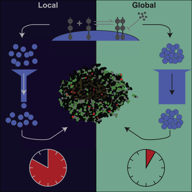
Graphical abstract

Highlights

• •Global method solves molecular dynamics in agent-based models of biological tissue
• •Speeds up simulations by orders of magnitude
• •Preserves spatial and temporal growth dynamics
• •Works with both spatial and phenotypic heterogeneity

In silico biology; Mathematical biosciences; Systems biology

Introduction

Living systems are intrinsically multiscale - biological components are tethered together in interconnected labyrinths that are dynamically changing in time and space (Dhurjati and Mahadevan, 2008). Multiscale mathematical models have been used as a conceptual framework to study such systems where, for example, biological components participate in an ongoing dialogue consisting of sending, receiving, and interpreting an elaborate set of molecular signals (Meier-Schellersheim et al., 2009). Of the variety of multiscale mathematical modeling approaches that exist, agent-based models (ABMs) have emerged as a powerful tool in both basic biology (Holcombe et al., 2012) and translational systems biology (An et al., 2009), which is a field that combines laboratory, clinical, and computational methods to develop effective strategies for controlling biological processes related to human health and translating these findings for rapid clinical application (Vodovotz and An, 2014).

An ABM describes populations as individuals or agents, each with its own set of properties and behaviors. In this way, these models are well-suited to capture the connectivity and heterogeneity in biological systems. The traditional method for incorporating the molecular level details of cell signaling and targeted therapeutics into ABMs involves solving systems of ordinary differential equations (ODEs) locally at each spatial location where a cell resides (Ghaffarizadeh et al., 2016; Wang et al., 2009; Cilfone et al., 2015). We will refer to this commonly used approach as the local method. As the number of cells increases, solving a system of ODEs for each agent significantly increases the computational costs and becomes prohibitive when simulating upwards of ${10}^5$ cells (Cilfone et al., 2015). However, even just one cubic centimeter of tissue will contain more than ${10}^8$ cells (Del Monte, 2009). To accurately capture biological processes at this scale in mathematical models will thus require the development of new theoretical and computational frameworks. To reduce the computational time and expense associated with the currently used local method described above, we introduce and validate a faster approach that we will refer to as the global method for simulating multiscale ABMs of interacting molecular and cellular systems (Figure 1).

Figure 1.

Methods cartoon

(A) Depiction of how the methods work. Both methods first update drug and receptor concentrations with short time steps. The local method splits the five biological processes among three differential equations which are solved in succession over each short time step. The global method packages all of this into a single ODE which is then solved using a stiff ODE solver. The output of both methods is then used to affect cell fate decisions before repeating the entire process.

(B) Two implementations of the global method. The first uses occupied and non-occupied regions to define dynamic regions within the microenvironment. The second uses geometrically-derived regions, for example distance from the blood vessel. In both implementations, the average concentration in each region is used to solve the reaction equations.

We take the molecular drivers of cancer growth and targeted molecular therapeutics as our test case to explain the similarities and differences between the local and global methods and to demonstrate the advantages of our simulation strategy. Translational systems biology and systems pharmacology are two examples of fields where approaches that incorporate agent-based modeling have been used to both broaden our understanding of cancer biology and improve our ability to treat cancer in the clinical setting (Norton et al., 2019). For example, in cancer therapeutics, multiscale ABMs have been used to investigate the impact of combined therapies on myeloma cell growth (Ji et al., 2017), to predict the effect of receptor tyrosine kinase inhibitor therapy in brain cancer (Sun et al., 2012), to help guide the rational design of complex therapeutic interventions that target the colorectal cancer microenvironment (Kather et al., 2017), and to provide a framework for predicting treatment/biomarker combinations in different cancer types (Gong et al., 2017). These models and others like them provide strong evidence for the using ABMs to predict disease progression and guide recommendations for therapeutic interventions (Anderson and Quaranta, 2008; Yankeelov et al., 2015).

Given that ABMs have many basic science and translational applications and that the primary focus of our test case is cancer biology, we will introduce and validate the global method with two models of cancer growth and targeted therapy (Figure 2). These two models lend themselves to two different implementations of the global method that are illustrative of the flexibility and extensibility of this method. The first is a fibroblast growth factor receptor 3 (FGFR3)-mediated bladder cancer and treatment. In this system, FGFR3 is mutated on the tumor cells, resulting in constitutive signaling that confers a fitness advantage (Casadei et al., 2019). A small-molecule inhibitor (SMI) of FGFR3–a therapy that has shown promise in clinical trials (Siegel et al., 2020; Casadei et al., 2019)–is administered to suppress tumor growth. As its name suggests, an SMI has a very small size with an atomic mass on the order of 100 Da (Arkin et al., 2014). This affects certain pharmacodynamic properties of these drugs, such as diffusion rates and elimination rates (Buchwald, 2010). In the local method, we observe that the FGFR3 signaling in the presence of the SMI quickly reaches a uniform quasi-equilibrium, and thus we implement the global method by viewing the entire tumor mass as belonging to a single region that changes with the tumor.

Figure 2.

Model cartoons

(A) Cartoon of the molecular interactions on the cell surface. The FGFR3 inhibitor binds to the domain within the cell to block activation of downstream effects on proliferation and apoptosis.

(B) A rendering of the model with 13,000 cells shortly after therapy. All cell fate decisions from the previous 9 h are shown. Cells in the first octant are removed to show the center of the tumor.

(C) The cell lineage model.

(D) Cartoon of the molecular interactions on the cell surface. Anti-IL-6R antibody also binds IL-6 in the same manner, but the effect is to block IL-6R signaling.

(E) A rendering of the model with 1,000 cells. All cell fate decisions from the previous 3 h are shown.

Viewing the global method as an approximation of the local method, we test the hypothesis that the output from the local and global methods agree. In the FGFR3 system, we look at the FGFR3 signaling in both methods. As we observe that the local method shows uniform effects across all tumor cells, we implement the global method with all tumor cells in a single, uniform region. As the effect of this pathway is on the growth dynamics of the cells, we develop a metric that we refer to as the expected growth rate (EGR) or the total expected growth (TEG) when it is integrated. It is a noise-free measurement of how much a population in an ABM will grow on average, which we use to make comparisons between the methods without needing to run many simulations. We also record the wall time, which is the time in the real world that the algorithm takes to go from start to finish, to compare the speed of the two methods. We also consider the wall time spent on the constituent parts of the algorithms to determine which modules are most responsible for the computational cost. We finally look at the signal-to-noise ratio in the local method to quantify the heterogeneity of drug penetrance and activity to compare against the uniform output of the global method. We explore the sensitivity of these results to the parameter values in the Supplement to show how these results generalize to other systems.

We then apply the global method to a second system that provides a richer study of the spatial dynamics of the molecules and agents. This system looks at the interleukin-6 (IL-6)-mediated, cancer-stem-cell-driven growth of head and neck squamous cell carcinoma (HNSCC) (Herzog et al., 2021). IL-6 is a cytokine that affects many cell processes, such as proliferation and survival, and it is commonly overexpressed in most cancer types (Krishnamurthy et al., 2014; ChoudharyMoaz et al., 2016). The therapeutic strategy considered for this case is a monoclonal antibody against IL-6R, which contrasts with the SMI described above as antibodies are larger and penetrate into the tumor differently. Both of these molecules are known to enter the tumor from blood vessels and have been observed to affect tumor cells based on their proximity to these blood vessels (Krishnamurthy et al., 2010). We thus implement the global method with the natural geometry this imposes on the tumor.

In the IL-6 system, the natural geometry imposed by the location of blood vessels leads us to implement the global method with multiple regions defined by their distance from the blood vessel. We still consider the cell signaling differences between the two methods, but focus more on the spatial distributions of the molecules and of the different cell phenotypes. In particular, we focus on the distributions of their distances from the blood vessel as well as the local densities near each cell type.

Results

The global method accurately and quickly reproduces the results of the local method in the FGFR3 model

The global method output matches the local method output

Our first goal is to establish the equivalence of these two methods in the FGFR3 model. We use each method 20 times to simulate a growing tumor that starts with 10,000 tumor cells and grows for 8 days, applying daily doses of anti-FGFR3 therapy starting on Day 1 and ending on Day 5, corresponding to a typical dosing schedule of FGFR3 inhibitor given only on weekdays (Hahn et al., 2017). The quantity of the dose is chosen to reflect the empirically observed concentration in systemic circulation immediately after a 75 mg/kg dose is administered to a mouse (Grünewald et al., 2019). We use a step size of $\text{Δ}t=6\text{min}$ for cell fate decisions and a step size of $\tau =0.6\text{min}$ in solving the local method. We choose $\text{Δ}t$ faster than event rates to get a higher resolution on the metrics we measure. The local method time step is chosen based on the diffusion and reaction rates.

In Figure 3, we see agreement between the methods on the population dynamics of the tumor cells and the EGR. The methods also agree in terms of both the underlying inhibitor concentrations and mean strength of signal (Figure S1). Comparing all runs to their collective average, we see both methods follow similar residual distributions (Figure 3A). The inset shows the actual population dynamics.

Figure 3.

Global method is comparable to the local method but with substantially reduced wall time

(A–E) 20 simulations of each method over 8 days, each starting with 10,000 tumor cells.

(A) Population dynamics of the tumor cells show as residuals from the mean number of tumor cells across all simulations using both methods. Inset shows actual population trajectories.

(B) EGR for each simulation.

(C) Difference in EGR.

(D) Percent difference in tumor size. Comparison between simulations shown in gray. Comparison using EGR shown in black.

(E) Wall time for each simulation, separated by the method used. Note the log scale on the x-axis.

(F and G) Seven different initial tumor sizes and the wall time need to simulate them for 8 days with each method.

(F) Wall time dependence on initial tumor size.

(G) Proportion of wall time spent solving reaction ODEs.

To sift through the noise, we compare the EGR (see STAR Methods) for all runs. As the differences in tumor size between the two methods are driven by the calculation of ${\varphi }_D$ which is then used to determine EGR, the close agreement observed in Figure 3A follows from the similarity in EGR for each simulation (Figure 3B). In fact, the differences in EGR are less than $1\times {10}^{-3}{\text{d}}^{-1}$ with the maximum difference occurring immediately on therapy and 12 h after therapy (Figure 3C). Note that in plots B-C, there is one line plotted for each trajectory, indicating minimal stochastic effects on EGR.

Having established the equivalence of these methods in the FGFR3 model, we next look at how long each of these runs takes. The local method takes approximately 100 times longer than the global method (Figure 3E). The difference in these wall times is solely attributable to how the two methods handle inhibitor dynamics.

The global method reduces the computational time by more than one order of magnitude

Because we are often interested in modeling more than 10,000 cells and because models tend to grow more cells throughout the simulation, we analyze how the wall time of the two methods increases with the initial number of tumor cells. We vary the initial tumor population between 50 and 50,000 cells and run the simulation for 8 days. Comparing the wall times of these simulations (Figure 3F), we see that the local method is slower than the global method by one to two orders of magnitude. To put this another way, at the same time the local method simulated 500 tumor cells, the global method could simulate 50,000 tumor cells.

To better understand why the local method takes longer to simulate, we time the simulations at several levels of granularity: the total time for a simulation, the time to advance the whole system $\text{Δ}t$, and the time spent solving each differential equation. We also determine the wall time spent on tasks common to both methods by computing the difference between the duration of a single update and the time spent solving all differential equations. We call these common tasks. The local method spends more than 90% of the wall time on molecular dynamics (Figure S2E) and less than 10% on common tasks (Figure S2D), independent of the size of the tumor. For the global method, by contrast, the proportion of wall time spent on common tasks approaches 1 as the tumor size grows while the proportion spent on molecular dynamics approaches 0 (Figures S2D and S2E). This gives further evidence that the difference in wall times between these two methods will only grow as the number of cells gets larger. This is because all of the growth in the global method’s wall time is attributable to common tasks, which make up less than 10% of the growth in the wall time for the local method.

We further isolate the time spent solving ODEs for each, that is, excluding the diffusion PDE in the local method. We see that across all tumor sizes, a large proportion of time is spent on solving ODEs and that this proportion grows with the tumor size as the tumor size increases in the local method, this part grows toward taking up all 87% of the wall time spent on molecular dynamics (Figure 3G). This indicates that the primary driver of the increased wall time for the local method is solving the set of ODEs, one for each tumor cell. By contrast, the global method spends relatively little time-solving ODEs and less so as the tumor grows.

Variability in the local method is predictable but inconsequential

To understand how the intercellular variability in cell signaling as determined in the local method could lead to differences between the two methods, we look at the level of noise in the local method. In understanding the noise, we use the signal-to-noise ratio (SNR), which we define here as the ratio of the mean (signal) to the SD(noise) of the ${\varphi }_D$ values for all the cells used for cell fate decisions in a single update step. In Figure 4A, we plot this curve on the same axes as the actual ${\varphi }_D$ values with the SNR values given on the right in the log scale. We restrict the time domain over which we plotted the SNR to $\left[\mathrm{1,6.875}\right]$ to bring into focus the fluctuations in SNR when the drug is in the system. These values are all at least 50 and can grow upwards of ${10}^4$ during the daily administration of the drug. This indicates that the SD of the ${\varphi }_D$ values is at most 4%, and as little as 0.01%, of their mean value.

Figure 4.

Noise in the local method is negligible and follows predictable patterns

(A) SNR overlaid with the signal (${\phi }_D$).

(B) SNR plotted against time as the previous therapy. Color indicates the strength of signal. Time points for panels (C) and (D) marked.

(C) A heatmap of free drug concentration in the TME during the saturation phase. Darker color indicates higher concentration. The highest concentration shown is only 0.08% higher than the lowest. The brown line indicates the boundary of the tumor spheroid.

(D) Similar to C but shown during the elimination phase. Note the reversal of the location of high concentration. The highest concentration shown is only 0.005% higher than the lowest.

The pattern of the SNR is also informative of drug penetrance and activity in the tumor microenvironment (TME) over the course of one treatment. As expected, the SNR drops immediately and precipitously on dose administration only to quickly rise back to ${10}^2$ within 1 h. After 1.5 h, a similar pattern occurs with a smaller drop and slower rise. These are the results of known phases in drug delivery into a TME (Thurber et al., 2008) and we lay these out in Figure 4B by plotting all SNR values against the time after the previous therapy, discarding those that occurred before therapy or more than one day after therapy. The first phase is the saturation of the tumor with the drug where cells located at the leading edge of the tumor initially have increased access to the drug owing to neighboring lattice points being unoccupied and thus not taking up any of the drugs. These cells, eventually, saturate and the drug can more freely diffuse from outside the tumor into the center restoring a large SNR. However, the drug in the systemic circulation is being rapidly cleared during this time and is, eventually, unable to continue to supply the TME with adequate levels of drug to maintain the saturation of the tumor cells. At this time, the balance shifts with the center of the tumor holding more drug (much of it bound to surface-bound FGFR3) and the cells on the leading edge find their unoccupied neighbors losing drug more rapidly as there are no cells to keep it bound up. Thus, the second phase begins and continues through the elimination of the drug in circulation and in the TME. The heatmaps in Figures 4C and 4D highlight this effect by showing the concentration of free inhibitor within the TME during each of these phases.

This leaves the question of when the largest impact of noise can occur. That is, we want to know not only when the SNR is high, but when the corresponding signal is also high. To re-frame this: high relative levels of noise are insufficient to determine if there will be a large impact on our simulations because, at low levels of signal, relatively high levels of noise would nonetheless have small effects on cell fate decisions. This is owing to the functional forms which link the intracellular signaling with cell fate decisions being approximately linear. Thus, the SD alone indicates how much the noise would affect cell fate decisions and tumor growth. In Figure S3, we see that the SD peaks around 20 min and 10 h after therapy.

The global method is robust to changes in parameters

A key question that remains is how the parameters governing our current model might be affecting the results here and thus, whether this technique can be extended to other models that consider different drugs, different tissues, and different molecular targets. In particular, we are studying an SMI in the FGFR3 model, which implies certain ranges for parameters governing distribution and diffusion that are qualitatively different from those governing, for example, antibodies (Jain and Stylianopoulos, 2010; Thurber et al., 2008). Similarly, the reaction rates of these drugs with their intended targets can vary across many orders of magnitude (Tassa et al., 2010), which will dictate how quickly free molecules of the drug are bound up and how much remains free to diffuse throughout the microenvironment (Thurber et al., 2008).

We consider two groups of three kinetic parameters each and sample each parameter over three orders of magnitude with a Latin hypercube. These two groups are pharmacokinetic parameters and reaction rate parameters. We show that the largest difference in EGR between the two methods is 0.003 days⁻¹ (Figure S5F) and $3\times {10}^{-3}$ d⁻¹ (Figure S10F), respectively. Over an eight day simulation, this results in at most a $0.3\text{\%}$ difference in expected tumor size for both sets (Figures S4B). The SNR is high throughout the simulation for most parameter values and follows similar temporal patterns as observed in Figure 4B (Figures S4D and S6D). See Figures S4–S11 for all these results.

In addition, we consider how the method performs when we vary the vascular assumptions and consider the case that the drug is an antibody. Results for these are shown in Figures S12–S14.

The global method preserves spatial information in the IL-6 model

Where the global method implementation for the FGFR3 model uses dynamic regions and has a single agent phenotype, the implementation in the IL-6 model takes advantage of the natural geometry imposed by the location of the blood vessels to define static regions. The model also has three cell phenotypes. We thus use this model to further explore the validity of the global method by focusing on the spatial arrangement of agents and the penetrance of the substrates into the microenvironment. We simulate two cohorts of tumors: one without aIL-6R and one with aIL-6R. Both cohorts consist of 20 runs with each of the local and global methods, censoring after 50 days of simulated time. All tumors are initialized with $\left(\mathrm{100,10,20}\right)$ instances of (stem, progenitor, TD) cells, uniformly randomly distributed throughout a $20\times 20\times 20$ lattice. In these simulations, we use a step size of $\text{Δ}t=60\text{min}$ for cell fate decisions and a step size of $\tau =0.1\text{min}$ in solving the local method. We selected $\text{Δ}t$ based on the timescale for the fastest-occurring agent event, that is, movement. The local method time step was chosen based on the diffusion and reaction rates in the microenvironment. The concentrations for the two substrates are chosen empirically so that there are both discernible effects on cell fate decisions and so that there would be spatial heterogeneity. See STAR Methods for additional model details and see Table S4 for parameter values used. We remark here that the two methods produced similar growth dynamics for each agent phenotype (Figures 5A and 6A), though there is considerably more inter-simulation noise owing to fewer agents and the variability in the effects of spatial location. We also remark here that the global method takes much less time than the local method (Figures 5B and 6B) in both cohorts. The difference is around an order of magnitude and, importantly, it is clear that as the number of agents grows, the wall time spent on ODEs increases faster. This means that larger simulations will see larger differences between the wall times of the two methods.

Figure 5.

Global method agrees with the local method in growth dynamics and spatial distributions without aIL-6R

20 simulations of each method over 50 days, each starting with $\left(\mathrm{100,10,20}\right)$ of (stem, progenitor, TD) cells. Shaded areas represent $\pm$ one SD of inter-simulation variability.

(A) Population dynamics by type.

(B) Wall times for each simulation, separated by the method used. Left panel: total wall time per simulation. Note the log scale on the x-axis. Middle panel: cumulative wall time spent on molecular dynamics. Right panel: wall time on a single update step plotted against the number of agents in that update step.

(C) Average normalized distance to the blood vessel for each cell type throughout the simulation.

(D) Average free IL-6 concentration throughout the simulation. Left panel: the average concentration in each $z=k$ plane throughout the simulation. Middle panel: the estimated concentration in the global method. Right panel: percent difference in IL-6 concentration between the two methods computed as ((Global/Local)-1) $\times$ 100%.

Figure 6.

Global method agrees with the local method in growth dynamics and spatial distributions with aIL-6R

See Figure 5. Panel (D) shows aIL-6R rather than IL-6.

The global method preserves substrate concentration throughout the tumor microenvironment

We first look at the substrate concentrations in the microenvironment under the two methods. As the IL-6 concentration is held constant at the blood vessel throughout the simulation, the system quickly reaches an equilibrium state with high IL-6 concentration near the blood vessel which decays to near 0 by the far boundary (Figure 5D). The global method overestimates the average free IL-6 in a single region by no more than 10% over the average concentration in that same region in the local method (Figure 5D, right panel). The largest relative difference occurs in the regions nearest the blood vessel, but not actually held at a fixed concentration. For aIL-6R, the system reaches a uniform quasi-equilibrium quickly, and this uniformity is maintained even as the concentration in systemic circulation decreases (Figure 6D). The global method underestimates the free aIL-6R concentration by about 0.05% in each region compared to the average concentration in the same region in the local method (Figure 6D, right panel). We also establish the agreement between the methods on the timescale of 12 h as the substrates converge on a quasi-equilibrium in the microenvironment, showing substrate concentrations at 1 min intervals (Figure S15).

The global method preserves agent spatial arrangement in the tumor microenvironment

We next look at the spatial arrangement of all agents by phenotype, specifically looking at the distance by type from the blood vessel. Snapshots at the end of one simulation with each method are shown for the cohort without (Figure 7A) and with (Figure 7D) aIL-6R. In the first cohort without aIL-6R, stem cells move closer to the blood vessel relative to their progenitor and TD counterparts, particularly around Day 20 in the simulation (Figure 5C). This behavior is preserved between the two methods (Figure 7B). With the introduction of aIL-6R, this difference between cell types disappears, and this, too, is preserved between the two methods (Figures 6C and 7E). We also look at the codensity (see STAR Methods) of each cell type, and find the two methods differ little on this local aspect of agent spatial arrangements (Figures 7C, 7F, S16, and S17).

Figure 7.

Global and local methods produce similar spatial arrangements of agents

(A–F) Comparisons are made between the methods without (A–C) and with (D–F) aIL-6R. Shaded areas represent ± one SD of inter-simulation variability.

(A) Snapshots of one simulation at Day 50 in both methods using the color and shape scheme of Figure 2.

(B) Percent differences of distance to blood vessels (BV) by type computed as ((Global/Local)-1) $\times$ 100%.

(C) Same as (B) but comparing codensity.

(D–F) Same as (A–C) but with aIL-6R.

Discussion

Our global method makes it possible to perform vastly more agent-based modeling simulations on more realistic tumor sizes, specifically, and on larger numbers of cells in living tissues more generally. This new approach will speed up every step of the process for building, parameterizing, validating, and predicting with ABMs. The magnitude of this speedup will allow for a deeper exploration of ABMs and allow for more robust predictions. Most agent-based mathematical/computational approaches for modeling molecular-level details in these large cellular systems can feasibly simulate no more than ${10}^6$ cells on a quad-core desktop workstation (Ghaffarizadeh et al., 2018). However, coordinated cellular assemblies in living tissues consist of billions of cells. Obtaining an integrated understanding of dynamic molecular and cellular processes for realistic numbers of cells requires the development of new theoretical and computational frameworks that can operate efficiently at these large scales. This is true across a broad range of fields within systems biology as just one milliliter in the human body contains the order of ${10}^9$ cells.

To reduce the computational time and expense associated with currently used methods, in this work we introduce and validate a faster approach for simulating multiscale ABMs of large interacting molecular and cellular systems. Such models have been used to study diseases (Bauer et al., 2009; Cilfone et al., 2013; Deisboeck et al., 2011), treatments (Hunt et al., 2013), and angiogenesis (Qutub et al., 2009). Our first test case is an ABM where molecular drivers influence cell proliferation and survival with a drug that targets these drivers. Our second test case looks at an ABM where there is additional geometric information that is incorporated in the implementation. Commonly used simulation strategies explicitly model all of the resulting signaling events individually, but at a computational cost that grows linearly with the number of cells.

Our first aim was to show that the global method accurately approximates the net effect of cell signaling by averaging over groups of cells. By comparing cell signaling, expected growth rate, molecular distributions, and proximity to blood vessels, we showed this to be the case. This work fits into the paradigm of tuneable resolution in which certain aspects of a detailed model are coarse-grained out in order to save computational resources (Cilfone et al., 2015). Tuneable resolution has been applied to replace computationally expensive differential equations with non-differential equations modules to speed up simulations while not sacrificing accuracy (Marino et al., 2011; Gong et al., 2014).

The natural critique of the global method is the lack of an intracellular signaling model for each cell that could more fully capture tissue heterogeneity. According to our results, the external signals that affect these intracellular signaling networks can be successfully approximated by locally constant (in space, not time) functions once one has some preliminary understanding of the dynamics of the system. As phenotypic variation within tissue often occurs on a discrete scale, for example, epithelial or mesenchymal (Dongre and Weinberg, 2019), stem or non-stem cells (Jilkine, 2019), activated or not (Bayani et al., 2020), the global method solves a single system of ODEs for each of these distinct phenotypes, as we did with the IL-6 model. Even when a model includes phenotypic heterogeneity along a continuous spectrum, for example, protein expression (Sha et al., 2020), thresholds are often introduced to create discrete phenotypes. When the cellular variability is owing to spatial location as in the IL-6 model, the global method can divide the microenvironment into geometrically-derived regions.

Another critique is that the global method could be further simplified by a quasi-steady state assumption that would be sufficient to determine the average cell signaling and the resulting effect on cell fate decisions. If the assumption is valid for a given system, then our method will still converge on the quasi-equilibrium without much additional computation cost, certainly not relative to the rest of the cost for simulating the ABM (see Figure 3G). It is also not obvious that all intracellular signaling networks will have an easily computable quasi-equilibrium. In such cases, numerical methods would be necessary to determine equilibria, stability, and basins of attraction, which raises the computational cost of a quasi-equilibrium assumption.

In a similar vein, our chosen models may appear so simple as to be approximated by a system of ODEs, which is by far less computationally expensive even than the global method. Two points are warranted here. First, the conversion of an ABM into a system of ODEs is an active field of research (Nardini et al., 2021). Second, and more importantly, ABMs are modular while ODEs are not. Additional modules can be added to these models, requiring no additional consideration of the global method so long as there are no direct interactions with the molecular layer. For example, the addition of immune cells in the FGFR3 model does not require any changes to the global method implementation as immune cells are not known to express FGFR3.

Our second aim was to reduce the computational cost of simulating ABMs, which we did by reducing the wall time by as much as a factor of 100. That is, simulating a tumor of the size used in mouse models (${10}^6$ cells) for twenty simulated days using the local method on a quad-core desktop workstation would take around four weeks; using the global method, it would take less than half a day. This moves us toward the goal of simulating at the giga-scale (${10}^9$ cells) (Montagud et al., 2021). The main cause for the speedup is reducing the number of reaction ODEs that need to be solved at each step from the number of tumor cells down to either one (in the FGFR3 implementation) or a constant number (in the IL-6 implementation). This step in the local method is embarrassingly parallel, meaning that using additional computing resources such as a high-performance computing (HPC) cluster could narrow the gap between these methods. However, the stochastic nature of ABMs necessitates running hundreds, if not thousands, of simulations to understand the distribution of possible behaviors across many parameter values. Thus, while this time difference could be narrowed to a single simulation, it nonetheless shows that the global method allows for greater exploration of the model.

Having established that the global method works and works faster with our particular model systems in mind, we looked at how the method would perform in other contexts. First, in the FGFR3 model, we showed that the variability in the strength of the signaling pathway in the local method was small relative to its mean, demonstrating that the spatial location of the tumor cells has little effect on the drug-inhibited intracellular signaling. Even under different vasculature assumptions, this remained the case. Then, we showed that all these results were robust under varying model parameters that will vary with different drugs and different targets. Finally, we considered the specific case of an antibody that targeted FGFR3 in the same way as the SMI. Although there is less agreement between the two methods, the pattern of the expected growth rate shows that the global method is viable for understanding this system.

Indeed, the utility of the global method is not in comparing it with the local method. Rather, we want to be comparing the efficacy of various dosing strategies or evaluating the effects of biological parameters on tissue fate. Although our goal here was to have it agree with the local method, that was only to produce confidence that we can study biological systems using our new and faster method. Hence, even in cases where the local and global methods have relatively more variability, for example, the case of an avascular tumor treated with a monoclonal antibody, we can still use the global method to predict the effects of different parameter values and dosing schedules. This is because the global method shows qualitatively similar effects of various molecules on a tissue.

We thus expect this method to open new opportunities across basic biology and translational systems biology for deeper understanding of ABMs with more cells. Many techniques already exist in the field for simplifying ABM simulation and analysis. Mean-field models reduce an ABM down to a system of differential equations allowing for faster simulations if not explicit mathematical analysis (Baker and Simpson, 2010; Chaplain et al., 2020). Compartment-based models (CBMs) keep the agent-based nature of ABMs while achieving speedups and/or increased numbers of cells per simulation by coarsening the lattice to house more cells in a single spatial location (Fadai et al., 2019). Other approaches have begun to use machine learning to build a neural network to handle intracellular signaling pathways (Cess and Finley, 2020). Our method adds to this in an important way by decreasing the computational cost of including cell signaling and targeted therapeutics.

While we applied the global method to a lattice-based ABM, we see no reason it cannot be extended to other types of ABMs that involve molecular-level dynamics that affect cell fate decisions. For example, an off-lattice model, such as PhysiCell (Ghaffarizadeh et al., 2018), could discretize the microenvironment into a lattice of voxels in which each lattice point could contain multiple agents. Then, in solving the differential equations governing the molecular layer, either implementation of the global method here could be used to speed up these computations. For vertex-based models or Cellular Potts Models, the need for high spatial resolution at the boundary of cells perhaps precludes the utility of the global method. However, if the purpose of such resolution is tied, for example, to cell-cell interactions and not molecular dynamics, one can connect the molecular level dynamics in a given voxel to the average across some subset of the microenvironment. We have not made attempts to test the global method in such models, but make these remarks here as suggestions for those interested in making such extensions of the method.

In the context of lattice-based models as we have looked at here, the global method does have room for improvements and future innovations. As one example, the assumption that IL-6 production by endothelial cells is constant over time can be adapted to situations where this source term varies over time (similar to anti-FGFR3 in that model) or even space (if drug concentration decreases along the length of a capillary). As another, stochastic signaling in the global method could be used to mimic the variability of cell signaling within the microenvironment. These perturbations can be derived from experiments that quantify the variability of cell signaling in a tissue both spatially and temporally. For example, if data showed that IL-6R signaling was dependent on distance from blood vessels but with quantifiable variability within regions defined by their distance from blood vessels, then the output of the global method can be perturbed to match these observations. When the effect of cell signaling is a discrete phenotypic change, the output of the global method could be used to define a probability of switching in much the same way as the machine learning approaches (Cess and Finley, 2020).

There are many other phenomena that have large effects on ABMs that could require special care to include in the global method framework. For example, insufficient access to oxygen and basic nutrients can cause dramatic changes at the cellular and tissue levels. In cancer, interstitial fluid pressure, enhanced permeability and retention, tortuous vasculature, and inhomogeneity of the extracellular matrix can all have effects on drug distribution and diffusion in ways that add heterogeneity to the microenvironment (Jain and Stylianopoulos, 2010; Shipley and Chapman, 2010; Thurber et al., 2008). Also, cellular interactions with the ECM or proximity to draining lymph nodes can also affect the system in a way that may require consideration before implementing the global method. We hope that the groundwork we have laid will provide some assurances that it would be worth the effort.

Indeed, we ourselves will be using this method to explore how best to administer a combination targeted and immunotherapy to bladder cancer with this FGFR3 mutation. In addition to using the global method for FGFR3 SMIs, we will also be using it to model the immunotherapy acting within the TME. This requires modifying the global method to include intercellular signaling. In using the global method, we significantly increase our capacity to analyze the model, test different treatment protocols, and inform clinical decisions.

Limitations of the study

The present study only applied the global method to two examples of ABMs, yet there are many different features of ABMs and the systems they aim to model that are not here considered. This includes biological features–such as intercellular signaling and the extracellular matrix–as well as platform features–such as off-lattice models or Cellular Potts models. It remains to be seen to what degree the success we have had here with these models can be carried over into ABMs that do have these features.

STAR★Methods

Key resources table

REAGENT or RESOURCE	SOURCE	IDENTIFIER
Software and algorithms
MATLAB	The MathWorks, Inc.	https://www.mathworks.com/products/MATLAB.html
FGFR3 and IL6 models	This paper; Zenodo	https://doi.org/10.5281/zenodo.6470845

Resource availability

Lead contact

Further information and requests for resources and reagents should be directed to and will be fulfilled by the lead contact, Trachette Jackson (tjacks@umich.edu).

Materials availability

This study did not generate new unique reagents.

Method details

We compare two methods–the local method and the global method–for updating cell signaling in a lattice-based, 3D ABM (Figure 1A). This involves solving differential equations with state variables corresponding to receptors, inhibitors, and their complexes over a time step of $\text{Δ}t$. A standard method couples an ODE for distribution, a partial differential equation (PDE) for diffusion, and a system of ODEs per tumor cell for reaction rates (Ghaffarizadeh et al., 2016). We contrast this with a new method that combines all these into a single system of ODEs. To achieve this, we average the local state variable concentrations in a given region and solve an ODE with these to be applied globally to all cells in this region. For this reason, we call these two methods the local and the global method, respectively. Their differences are outlined in Table S1.

We first study the relationship between these two methods using an ABM of bladder cancer in which the tumor cells have acquired a mutation in the FGFR3 gene resulting in ligand-independent dimerization and thus have constitutive signaling along this pathway (Casadei et al., 2019) (Figure 2A). The tumor cells exist on a 3D lattice proliferating and undergoing apoptosis with rates of both events mediated by this FGFR3 signaling. The strength of this signal is the single means by which the two methods affect tumor growth. Additionally, we model the treatment of these in silico tumors with an SMI of FGFR3. Details of the FGFR3 ABM are included below.

To test our method in a new setting with richer spatial dynamics, we study the relationship between these two methods in an on-lattice, 3D ABM of IL-6-mediated tumor growth. The tumor in this ABM includes a cell-lineage model in which cancer cells can undergo successive rounds of differentiation starting from a stem-like state to a non-proliferative terminally differentiated (TD) state (Nazari et al., 2018). The tumor cells in this model also exist on a 3D lattice where they proliferate, undergo apoptosis, and also can engage in random movement. The rates of apoptosis for all cell types as well the self-renewal rate of cancer stem cells (Figure 2C) are affected by IL-6R signaling. We also model the treatment of a monoclonal antibody against IL-6R, aIL-6R, to observe the effects on the validity of the global method when larger therapeutic agents are simulated. Details of the IL-6 ABM are included below.

Here, we proceed by describing the differential equations that govern these two methods, outlining the ABM dynamics for each model, and introducing a new metric we use to compare them.

The local method

The local method splits the dynamics in the FGFR3 model into three differential equations–the diffusion dynamics (Equation 1), the distribution dynamics (Equation 2), and the reaction dynamics (Equation 5)–solving each in turn for a short duration $\tau \le \text{Δ}t$. The same split happens for the IL-6 model with those equations found in their corresponding place below (Equations 1, 3, and 7). These calculations are repeated until the molecular components of the system have been advanced by $\text{Δ}t$. This is similar to what others have done (Ghaffarizadeh et al., 2016). For simplicity, we will identify the start and end of each of these updates by $t=0$ and $t=\tau$, respectively. We then use the final concentration of the complex of interest to compute the fractional occupancy on each tumor cell x, which we call ${\varphi }_D\left(x\right)$ in both models for simplicity. See below for the effects of this quantity on cell fate decisions in the FGFR3 model and see below for the effects on the IL-6 model.

Local method: Diffusion

The diffusion equation describes the evolution of a substrate concentration in the microenvironment, $C\left(t,\mathbf{x}\right)$ or simply C. Only diffusion, D, and degradation, ${\lambda }_2$, are included in this equation. This PDE is solved over the microenvironment, denoted $\text{Ω}$, which is a rectangular prism containing the tumor and some surrounding tissue in our models. By default, we use a Neumann boundary condition, reflecting a far-field approximation that assumes the concentration of the substrate is approximately uniform far from the microenvironment of interest. We solve Equation 1 by using the locally one-dimensional method (LOD), splitting the Laplacian into three parts, one for each spatial direction. If a Dirichlet condition is required, which we do for IL-6 in the IL-6 model, then after each iteration in the LOD algorithm, we impose the Dirichlet condition at those lattice points.

$$\frac{\partial C}{\partial t}=D{\nabla }^{2}C-{\lambda }_{2}C,\frac{\partial C}{\partial \mathbf{n}}=0\text{on}\partial \text{Ω}$$ (Equation 1)

where $\mathbf{n}$ is the outward facing normal vector to $\partial \text{Ω}$.

Local method: Pharmacokinetics

Some substrates follow a PK model that connects concentrations of the substrate across multiple compartments of an organism. In cases where the substrate follows such a model, drugs being a typical example, we make this connection in the local method by adding source terms at the lattice sites that are adjacent to blood vessels. In the FGFR3 model, the distribution terms (Equation 2) follow a simplified two-compartment model that accounts for systemic elimination, influx into the TME, and degradation within the TME. The concentration of drug in the systemic circulation is represented by $C_{\text{sys}}\left(t\right)$ or simply $C_{\text{sys}}$. The additional drug concentration flowing into the TME is represented by $C_{\text{new}}$. At the end of this step, we add the new drug concentration to the updated old drug concentration, assuming that the drug entered the TME at all points equally. That is, we update the value of $C\left(\tau ,\mathbf{x}\right)$ to now be $C\left(\tau ,\mathbf{x}\right)+C_{\text{new}}\left(\tau \right)$. We use ${\lambda }_1$ to represent the rate of systemic elimination of the drug and $k_{12}$ to represent the rate of influx of the drug into the TME. We assume that the drug in circulation undergoes a monophasic elimination as is consistent with experiments using FGFR3 inhibitors (Grünewald et al., 2019). This means that the effects of distribution and redistribution on the systemic concentration can be reasonably approximated by a single elimination term for $C_{\text{sys}}$.

$$\begin{array}{l}\frac{d{C}_{\text{sys}}}{dt}=-{\lambda }_1{C}_{\text{sys}}\\ \frac{d{C}_{\text{new}}}{dt}=k_{12}{C}_{\text{sys}}-{\lambda }_2{C}_{\text{new}},C_{\text{new}}\left(0\right)=0\end{array}$$ (Equation 2)

We also consider the case where the tumor is not so well-vascularized that the drug enters at all points in the TME. This is important to consider given that it is well-known that tumor vasculature is often aberrant and highly variable even within a single tumor (Forster et al., 2017). It is also possible that a nascent tumor, such as a micrometastasis, is poorly vascularized or lacks vasculature all together (Bailey-Downs et al., 2014). We thus consider two additional assumptions about how blood vessels may be present in the TME. First, we consider the case of a several blood vessels running in a parallel lines through the tumor. We space these out on a lattice so that neighboring blood vessels are 400 μm apart to match the observation that all cells are within 200 μm of a blood vessel. Second, we consider the case that no blood vessels are in the tumor and instead drug enters the TME exclusively through points outside the tumor. These cases can be understood as a “normally” vascularized tumor and an avascular tumor. Our original assumption of drug entering the entire TME can then be understood as a “maximally vascularized” tumor and we can arrange these on a spectrum from most to least vascularized in this order: maximally vascularized, vascularized, avascular. In each of these new assumptions, we scale the dosing so that all simulated tumors receive approximately the same total amount of drug. In these cases, we simply only update the substrate concentrations at lattice sites next to the blood vessels to $C\left(\tau ,\mathbf{x}\right)+C_{\text{new}}\left(\tau \right)$.

In modeling the antibody in the IL-6 system, we use a three-compartment model that accounts for inter-compartmental clearance and redistribution in addition to the above-mentioned terms in the FGFR3 model. The reason for the extra compartment is because it gives rise to a biphasic elimination profile. In implementing this model, the PK dynamics were solved before the diffusion dynamics and so no consideration is needed for degradation of the newly-influxed substrate. This is evidence of the flexibility of the splitting and ordering of these equations that others have done (Ghaffarizadeh et al., 2016). Altogether, the PK model for aIL-6R is given by Equation 3. Here, $A_{\text{bv}}$ is the concentration at perivascular lattice sites in the TME, $A_{\text{sys}}$ is the concentration of aIL-6R in systemic circulation, and $A_p$ is the concentration in the peripheral compartment. Note that in this model, the substrate is entering only at certain lattice sites (perivascular sites) and not the entire TME as we initially assume in the FGFR3 model. Also, $A_p$ has no direct connection with the concentration in the TME.

$$\begin{array}{l}\frac{d{A}_{\text{bv}}}{dt}=e\cdot \left(A_{\text{sys}}-A_{\text{bv}}\right)\\ \frac{d{A}_{\text{sys}}}{dt}=-{\lambda }_1{A}_{\text{sys}}+k_{12}\left(A_p-A_{\text{sys}}\right)\\ \frac{d{A}_p}{dt}=k_{21}\left(A_{\text{sys}}-A_p\right)\end{array}$$ (Equation 3)

Local method: Reactions

Finally, we solve the reaction equation for each tumor cell, sampling from C to determine the inhibitor concentration accessible to each cell. In the FGFR3 model, the system of ODEs in Equation 5 has six dependent variables: R is for FGFR3 monomers, $D_A$ is for active FGFR3 dimers, C is for FGFR3 inhibitor, $R^C$ is for the monomer-inhibitor complex, $D_A^C$ is for the active dimer-inhibitor complex, and $D^C$ is for the monomer-inhibitor dimer. All variables are defined as local concentrations at each tumor cell. We note that we could be explicit and write $C\left(t,{\mathbf{x}}_i\right)$ for the inhibitor concentration near tumor cell i, which is located at ${\mathbf{x}}_i$, but we instead use C here as the context makes the meaning clear. The reactions and their rates are in Equation 4. All the terms in Equation 5 arise from reaction rates following the law of mass action with appropriate stoichiometric coefficients.

$$\begin{array}{l}2R\underset{k_f}{\overset{k_r}{\rightleftharpoons }}{D}_A\left(\text{monomer dimerization}\right)\\ D_A\stackrel{k_p}{\to }2R\left(\text{internalization and recycling}\right)\\ R+C\underset{k_{\text{off}}^R}{\overset{k_{\text{on}}^R}{\rightleftharpoons }}{R}^C\left(\text{inhibitor binding monomer}\right)\\ D_A+C\underset{k_{\text{off}}^D}{\overset{k_{\text{on}}^D}{\rightleftharpoons }}{D}_A^C\left(\text{inhibitor binding dimer}\right)\\ 2R^C\underset{k_f}{\overset{k_r}{\rightleftharpoons }}{D}^C(\text{monomer}-\text{inhibitor dimerization})\\ D^C\stackrel{k_p}{\to }2R^C\left(\text{internalization and recycling}\right)\end{array}$$ (Equation 4)

$$\begin{array}{l}\frac{dR}{dt}=-2k_f{R}^2+2k_r{D}_A+2k_p{D}_A-k_{\text{on}}^{R}RC+k_{\text{off}}^R{R}^C\\ \frac{d{D}_A}{dt}=k_f{R}^2-k_r{D}_A-k_p{D}_A-k_{\text{on}}^D{D}_{A}C+k_{\text{off}}^D{D}_A^C\\ \frac{dC}{dt}=-k_{\text{on}}^{R}RC+k_{\text{off}}^R{R}^C-k_{\text{on}}^D{D}_{A}C+k_{\text{off}}^D{D}_A^C\\ \frac{d{R}^C}{dt}=k_{\text{on}}^{R}RC-k_{\text{off}}^R{R}^C-2k_f{\left(R^C\right)}^2+2k_r{D}^C+2k_p{D}^C\\ \frac{d{D}_A^C}{dt}=k_{\text{on}}^D{D}_{A}C-k_{\text{off}}^D{D}_A^C\\ \frac{d{D}^C}{dt}=k_f{\left(R^C\right)}^2-k_r{D}^C-k_p{D}^C\end{array}$$ (Equation 5)

In the IL-6 model, the system of ODEs in Equation 7 has five dependent variables: R is for IL-6R, C is for free IL-6, $R^C$ is for IL-6-IL-6R complexes, A is for aIL-6R, and $R^A$ is for the IL-6-aIL-6R complexes. Again, all variables are defined as local concentrations at each tumor cell. We also note here that we could be explicit and write $C\left(t,{\mathbf{x}}_i\right)$ and $A\left(t,{\mathbf{x}}_i\right)$ for the IL-6 and aIL-6R concentrations, respectively, near tumor cell i, which is located at ${\mathbf{x}}_i$, but we instead use C and A here as the context makes the meaning clear. The reactions and their rates are in Equation 6. All the terms in Equation 7 arise from reaction rates following the law of mass action with appropriate stoichiometric coefficients.

$$\begin{array}{l}R+C\underset{k_f}{\overset{k_r}{\rightleftharpoons }}{R}^C(\text{IL}-6-\text{IL}-6\text{R}\text{reaction})\\ R+A\underset{k_f^A}{\overset{k_r^A}{\rightleftharpoons }}{R}^A(\text{IL}-6\text{R}-\text{aIL}-6\text{R}\text{reaction})\end{array}$$ (Equation 6)

$$\begin{array}{l}\frac{dR}{dt}=-k_{f}RC+k_r{R}^C-k_f^{A}RA+k_r^A{R}^A\\ \frac{dC}{dt}=-k_{f}RC+k_r{R}^C\\ \frac{d{R}^C}{dt}=k_{f}RC-k_r{R}^C\\ \frac{dA}{dt}=-k_f^{A}RA+k_r^A{R}^A\\ \frac{d{R}^A}{dt}=k_f^{A}RA-k_r^A{R}^A\end{array}$$ (Equation 7)

The global method

The global method solves the differential equations described above for the local method, but does so by combining them into a single system of ODEs and solving them all at once. To do this, we first divide the TME into two or more regions over which molecular state variables will be averaged to solve the equations. This system of equations is solved using a MATLAB solver, ode15s. The reaction equations can exhibit some stiffness, and that is why we use this particular solver. The output of this process is applied to each tumor cell. In the IL-6 model, the region and type of the tumor cell are considered in applying this output. Consequently, two cells of the same type and in the same region experience identical effects of the substrate on their cell fate decisions.

The global method with dynamic regions: FGFR3 model

In the FGFR3 model, the global method will assign a single vector of receptor, inhibitor, and complex concentrations to each tumor cell as well as an average concentration at all lattice points not occupied by a tumor cell. To do this, we define two disjoint regions of the TME: the tumor-occupied volume (TOV) and the ambient space (AMB). We assume that the drug concentrations in each of these regions can be approximated by their average concentrations. These regions are dynamic in that they change over the course of a single simulation as tumor cells proliferate and die.

In connecting the concentrations of these two regions for diffusion calculations, we need to define their volumes. For simplicity, we use cells as our unit of volume with each lattice location representing one unit. The volume of the TOV is then simply the number of tumor cells, $N_T$. The volume of the ambient space is the volume of the TME minus the volume of the TOV. We denote the volumes of these two disjoint subsets of the TME as $V_{\text{TOV}}$ and $V_{\text{AMB}}$, respectively, and similarly define $V_{\text{TME}}=V_{\text{TOV}}+V_{\text{AMB}}$.

The global method with geometrically-derived regions: IL-6 model

In a context where there is a clear geometry to the distribution of a substrate in the TME, the global method can be modified to better reflect that reality. For example, in the IL-6-mediated cancer growth model, endothelial cells are known to produce large amounts of IL-6, in addition to being the entry point of antibodies into the TME. It follows that the distance to the blood vessel of a given cell informs how much substrate the cell can react with. Thus, in the IL-6 model we divide the TME into static regions by the distance of the lattice site to the nearest blood vessel. In this work, we shall place the blood vessel on the “bottom” boundary ($z=z_{\text{min}}$) and define the regions as one cell thick planes each defined by their distance from the blood vessel. It is possible to view each such plane as a TME with occupied and non-occupied volumes as above, giving it dynamic subregions, but we shall here assume that each region is well-mixed, in other words that it has a uniform density of each substrate throughout.

Global method: Diffusion

We now describe how the global method handles diffusion. We start with the diffusion term of the PDE in Equation 1, discretize it using finite differences, and assume the average concentrations in each of the neighboring locations to compute the rate of change in the central location. Defining some terms, let u be the concentration of inhibitor in the TME and let $u_{jkl}^i$ be the discretization of u at time step i and at location $\left(x_j,y_k,z_l\right)$ on the lattice with a uniform step size of h. Let v and w be the average concentrations in the TOV and ambient space, respectively. Let p be the proportion of the TME that the TOV occupies and let $q=1-p$ be the proportion the ambient space occupies. Using the notation from above, we can also write $p=V_{\text{TOV}}/V_{\text{TME}}$ and $q=V_{\text{AMB}}/V_{\text{TME}}$. Then, a standard finite difference scheme for the Laplacian gives

$$u_t={\nabla }^{2}u\approx \frac{u_{j-1kl}^i-2u_{jkl}^i+u_{j+1kl}^i}{h^2}+\frac{u_{jk-1l}^i-2u_{jkl}^i+u_{jk+1l}^i}{h^2}+\frac{u_{jkl-1}^i-2u_{jkl}^i+u_{jkl+1}^i}{h^2}$$ (Equation 8)

A first approach, and one we make in the FGFR3 model, is to assume that the neighboring locations in the lattice being in the TOV or ambient space is independent of which one the central point is. That is, the expected concentration of, for example, $u_{j-1kl}^i=pv+qw$. Thus, if there is a tumor cell at $\left(x_j,y_k,z_l\right)$, then

$$\frac{u_{jkl}^{i+1}-u_{jkl}^i}{\text{Δ}t}=\frac{3}{h^2}\left(2\left(pv+qw\right)-2v\right)=\frac{6}{h^2}\left(\left(p-1\right)v+qw\right)=\frac{6q}{h^2}\left(w-v\right)$$ (Equation 9)

Similarly, if there is no tumor cell at $\left(x_j,y_k,z_l\right)$, then

$$\frac{u_{jkl}^{i+1}-u_{jkl}^i}{\text{Δ}t}=\frac{6p}{h^2}\left(v-w\right)$$ (Equation 10)

The expressions in Equations 9 and 10 are then added to $d{C}_{\text{TOV}}/dt$ and $d{C}_{\text{AMB}}/dt$.

A second approach, and one we take in the IL-6 model, is to calculate the proportion of neighbors that belong to a given region and use this in place of p and q above. In the IL-6 model, the regions are square regions that are one cell thick, and so $1/6$ neighbors are in each of the regions above and below a given region and the remaining $2/3$ are in the same region. At a lattice site on the boundary of the lattice where a Neumann condition is imposed, we assume that its neighbors are in its region. We remark here that this computation of neighbors could be done in the dynamic regions of the FGFR3 model by computing the proportion of neighboring lattice sites to tumor cells that are occupied or not. If we let $C_i$ represent the concentration in region i and $p_{ij}$ be the proportion of region i neighbors in region j, then the effect of diffusion on region i is given by

$$\frac{d{C}_i}{dt}=\sum _j\frac{6p_{ij}}{h^2}\left(C_j-C_i\right)$$ (Equation 11)

Both of these approaches can be understood as weighted averages of the concentration differences between both/all the regions, multiplied by the factor $2d/h^2$, where d here is the number of spatial dimensions in the simulation.

Global method: Pharmacokinetics

In the FGFR3 model, we initially assume that the drug enters the TME at all points equally. Thus, the pharmacokinetics are captured by adding a $k_{12}{C}_{\text{sys}}$ term to the rates of change for both $C_{\text{TOV}}$ and $C_{\text{AMB}}$. Since the reactions are all solved at once, we do not need to create a new variable $C_{\text{new}}$ to track newly-extravasated drug in the TME. The PK reactions in the FGFR3 model are then given in Equation 12.

$$\begin{array}{l}\frac{d{C}_{\text{TOV}}}{dt}=k_{12}{C}_{\text{sys}}\\ \frac{d{C}_{\text{AMB}}}{dt}=k_{12}{C}_{\text{sys}}\\ \frac{d{C}_{\text{sys}}}{dt}=-{\lambda }_1{C}_{\text{sys}}\end{array}$$ (Equation 12)

When we consider the other vascularization possibilities described above in the FGFR3 model, we multiply the rates for $d{C}_{\text{TOV}}/dt$ and $d{C}_{\text{AMB}}/dt$ in Equation 12 by the proportion of their respective regions that contain blood vessels.

In the IL-6 model, we assume that only one region, Region 1, is perivascular, we only add a PK term for this region in the aIL-6R dynamics (Equation 13). Note, IL-6 does not have a PK component; it enters the TME via a Dirichlet condition imposed on perivascular sites.

$$\begin{array}{l}\frac{d{A}_1}{dt}=e\cdot \left(A_{\text{sys}}-A_1\right)\\ \frac{d{A}_{\text{sys}}}{dt}=k_{12}\left(A_p-A_{\text{sys}}\right)\\ \frac{d{A}_p}{dt}=k_{21}\left(A_{\text{sys}}-A_p\right)\end{array}$$ (Equation 13)

Global method: Reactions

In the FGFR3 model, the reaction equations are solved by using the average across all the molecular state variables and in the TOV. That is, the average concentrations are used as the state variables in solving Equation 5.

For the IL-6 model, the different cell types react differently with the substrates due to assumptions about how many IL-6R each has (see $R_T$ in Table S4). So, we set $R_{ik}$ to represent the average concentration of IL-6R on cell type k in region i (where $k=\mathrm{1,2,3}$ stands for the three cell types in the cell lineage model), and similarly for other cell bound complexes. Additionally, since the molecular reactions only occur in a subset of each region, we must weight the contributions to the average concentration within the region accordingly. Letting $q_{ik}$ represent the proportion of region i that has a cell of type k, these give weights for each region for the effects of the reaction on the average concentration. Then, the full set of reaction equations is given by

$$\begin{array}{l}\frac{d{R}_{ik}}{dt}=-k_f{R}_{ik}{C}_i+k_r{R}_{ik}^C-k_f^A{R}_{ik}{A}_{ik}+k_r^A{R}_{ik}^A\\ \frac{d{C}_i}{dt}=-k_f\sum _{k=1}^3{q}_{ik}{R}_{ik}{C}_i+k_r\sum _{k=1}^3{q}_{ik}{R}_{ik}^C\\ \frac{d{R}_{ik}^C}{dt}=k_f{R}_{ik}{C}_i-k_r{R}_{ik}^C\\ \frac{d{A}_i}{dt}=-k_f\sum _{k=1}^3{q}_{ik}{R}_{ik}{A}_i+k_r\sum _{k=1}^3{q}_{ik}{R}_{ik}^C\\ \frac{d{R}_{ik}^A}{dt}=k_f^A{R}_{ik}{A}_i-k_r^A{R}_{ik}^A\end{array}$$ (Equation 14)

FGFR3 agent-based model

Agents in the FGFR3 model exist on a 3D lattice. The agents are initialized randomly with lattice sites chosen randomly with weights that decay based on their distance from the origin. Once the agent locations are decided, a box is created around all the tumor cells and that defines the lattice for the simulation. The agents always occupy a single lattice site. The volume of agents is assumed to be constant and held at the volume of one lattice site, $w^3$. All parameter values for this model are in Table S2. The parameters values that change when considering an anti-FGFR3 antibody in place of an SMI are in Table S3.

FGFR3 model: Population updates

Common to both methods is how the populations update. The simulation is discretized into uniform time steps of $\text{Δ}t\le 12\text{h}$. During each step, every tumor cell has a probability, $p_{\text{active}}\left(x\right)$, to make a cell fate decision either to proliferate or to undergo apoptosis, which we consider mutually exclusive events during one time step. Otherwise, the tumor cell rests. These probabilities are computed using the formula:

$$p_i\left(x\right)=r_i\left(x\right)\text{Δ}t,i=\text{proliferation},\text{apoptosis}$$ (Equation 15)

where i indexes the events, $x\in \mathcal{T}$ represents individual tumor cells, and $r_i$ is the cell-specific rate of each process defined below. This is a first-order approximation of the exponential distribution which is appropriate here because our time step is small. For larger time steps, we would need to instead use $p_i\left(x\right)=1-\text{exp}\left(-r_i\text{Δ}t\right)$. At each step, we check that that the sum of all these probabilities does not exceed 1, i.e.

$$p_{\text{active}}\left(x\right)=\sum _i{p}_i\left(x\right)\le 1,\forall x\in \mathcal{T}$$ (Equation 16)

If this sum does exceed one, we can simply decrease the time step, $\text{Δ}t$, to address this. To choose the fate of each cell, we take a random draw $s\left(x\right)\sim \mathcal{U}\left(\mathrm{0,1}\right)$ for each $x\in \mathcal{T}$ and compare this to the vector of cumulative sums of these probabilities, $S\left(x\right)$, choosing the smallest index j satisfying $s\left(x\right)<S{\left(x\right)}_j$ as the choice for x. Once all cells have a fate chosen, we shuffle the order in which to carry out these updates to avoid unintentionally biasing the system in some way due to the biologically meaningless ordering of cells in the tumor.

FGFR3 model: Fractional occupancy

Every tumor cell has FGFR3 receptors. These receptors dimerize as governed by the reaction equations found in Equation 5 with ramifications for cell fate decisions as covered in subsequent sections. Otherwise, these receptors will only interact with inhibitor molecules. We define the active FGFR3 dimer fractional occupancy by

$${\varphi }_D\left(x\right)=\frac{D_A\left(x\right)}{R_T}$$ (Equation 17)

where $D_A\left(x\right)$ represents the concentration of active dimers on tumor cell x and $R_T$ is a constant representing the concentration of all FGFR3 receptors, regardless of their state, on each tumor cell. Due to there being, by definition, at most half as many dimers as monomers, we know that at throughout the simulation

$${\varphi }_D\left(x\right)=\frac{D_A\left(x\right)}{R_T}\le \frac{1}{2}$$ (Equation 18)

FGFR3 model: Proliferation

The tumor cells proliferate at a base rate of ${\alpha }_1$ that is increased by FGFR3 signaling. This increase is dependent upon ${\varphi }_D\left(x\right)$ and the constant ${\alpha }_2$ by

$$r_{\text{proliferation}}\left(x\right)={\alpha }_1+{\alpha }_2{\varphi }_D\left(x\right)$$ (Equation 19)

When a cell is assigned the fate of proliferation, if there are $\le O_{\text{max}}^{\text{prolif}}$ open lattice spots in the Moore neighborhood around a tumor cell, we prohibit proliferation to reflect density-dependent proliferation. If there are sufficient open spots, then these are weighted by the reciprocal of their distance in the ${\ell }_1$ norm (the taxicab metric) from the tumor cell and one is selected randomly based on these weightings for the new cell to be placed in. Reflecting boundary conditions are also imposed so cells on the boundary view neighboring sites that are off the lattice as occupied.

There are two important ways we change this base rate based on whether a cell has recently proliferated. The first is that a cell must wait a minimum of $L_{G0}$ hours between proliferations. Thus, if it has not been $L_{G0}$ hours since the last proliferation for x, then $r_{\text{proliferation}}\left(x\right)=0$. When the cell does proliferate, it is assumed that it happens at a random time, chosen uniformly over the update interval. Second, if this period expires during the update step, then the remaining time is used in place of $\text{Δ}t$ for cell x. That is, if the cell must still wait $w<\text{Δ}t$ hours at the start of the update, then $\text{Δ}t$ in Equation 15 is replaced by $\text{Δ}t-w$ for the proliferation probability of cell x. Together, these make the proliferations more realistic–not allowing the same cell to proliferate multiple times in a short time interval–and creating greater consistency between different choices of $\text{Δ}t$.

We must then determine what receptor concentrations to assign to the two new daughter cells. When $\text{Δ}t$ is small, we cannot assume that the reactions are at equilibrium and so their initial conditions will matter. We assume that all complexes on the original cell are split evenly between the two cells, i.e. each has half the original concentration. Then, enough FGFR3 monomer is assigned so the total concentration of FGFR3 in all forms is $R_T$. The two methods differ slightly in handling the free inhibitor at this step because of the dynamic regions in this implementation of the global method. The local method explicitly tracks this concentration throughout the entire TME and this value is used for each daughter cell. The global method updates the average TOV free inhibitor concentration by taking a weighted average of this value with the concentration in the AMB. The weight for TOV concentration is the previous number of tumor cells (representing the previous volume of the TOV) and the weight for the AMB is one (representing the volume of the newly added cell). The average concentration in the AMB is unaffected by this process.

FGFR3 model: Apoptosis

The tumor cells undergo apoptosis at a base rate δ that is decreased by FGFR3 signaling. This decrease is also dependent on ${\varphi }_D\left(x\right)$ and the constant γ:

$$r_{\text{apoptosis}}\left(x\right)=\frac{\delta }{1+{\varphi }_D\left(x\right)/\gamma }$$ (Equation 20)

After all the cell fates are resolved, the apoptotic cells are removed from the lattice, freeing up their locations for new tumor cells to proliferate into on subsequent steps.

Additionally, in the global method we update the concentration of free inhibitor in the AMB after each apoptosis, corresponding to a new location no longer occupied by a tumor cell. To do this, similarly to the proliferation step, we update this concentration by taking the weighted average of this value with the average concentration in the TOV. The weight assigned to the AMB concentration is the volume of the AMB (computed as the difference between the total number of lattice points and the previous size of the tumor). The weight assigned to the TOV is the number of apoptotic cells removed, corresponding to the volume of the newly unoccupied locations.

IL-6 agent-based model

In the IL-6 model, tumor cells also exist on a 3D with reflecting boundary conditions and a maximum of one cell per lattice site. The agents are initialized uniformly distributed on a $20\times 20\times 20$ lattice.

IL-6 model: Cell lineage

Cancer cells are one of three distinct phenotypes: cancer stem cells, progenitor cells, and terminally differentiated cells (TDs). As shown in Figure 2C, cancer stem cells can undergo both symmetric and asymmetric division. The former increments the stem cell compartment by one while the latter increases the progenitor cell compartment by one. Progenitor cells undergo w rounds of transient amplification where their division results in an additional progenitor cell. After these w proliferations, their next division produces two TD cells, which are non-proliferative.

IL-6 model: Population updates

The cells in the IL-6 model follow the same algorithm as those in the FGFR3 model for choosing their cell fate decisions in each update step, using the exact value of the exponential distribution rather than the approximation in Equation 15. In addition to proliferation and apoptosis, cells in this model can also undergo random movement in a Moore neighborhood. As with proliferation, reflecting boundary conditions are imposed to prevent cells from leaving the lattice.

IL-6 model: Fractional occupancy

Analogous to ${\varphi }_D$ above in the FGFR3 model, the fractional occupancy of IL-6R on tumor cells is used to mediate rates, and thus probabilities, of certain cell fate decisions. Here, ${\varphi }_D$ is the proportion of IL-6R on a given tumor cell that is bound to IL-6, i.e. it is given by

$${\varphi }_D\left(x\right)=\frac{R^C\left(x\right)}{R_T\left(x\right)}$$ (Equation 21)

where $R_T\left(x\right)$ is the total IL-6R on cell x, which varies by cell type according to Table S4.

IL-6 model: Proliferation

The resultant cell types of proliferation are described above under cell lineages. The only aspect of this affected by ${\varphi }_D$ is the probability that a stem cell undergoes symmetric division instead of asymmetric division. Higher ${\varphi }_D$ values result in higher probabilities of symmetric division. In addition, there is a negative feedback from the stem cell population on this self-renewal rate. This probability, $P_S$ is given in Equation 22 where S is the number of stem cells in the model.

$$\begin{array}{l}{P}_S\left(S,{\varphi }_D\right)=\frac{\left(P_{S_{\text{max}}}-P_{S_{\text{min}}}\left({\varphi }_D\right)\right)P_{N_s}^n}{P_{N_s}^n+S^n}+P_{S_{\text{min}}}\left({\varphi }_D\right)\\ P_{S_{\text{min}}}\left({\varphi }_D\right)={\mu }_S\left(P_{S_{\text{max}}}-P_{S_{\text{min}}}^{\text{∗}}\right){\varphi }_D+P_{S_{\text{min}}}^{\text{∗}}\end{array}$$ (Equation 22)

See (Nazari et al., 2018) for a full explanation of these expressions.

IL-6 model: Apoptosis

As in the FGFR3 model, apoptosis rates decrease for all cell types as ${\varphi }_D$ increases. The rate of apoptosis in this context is modeled by the exact same Hill-type function in Equation 20 with parameter values chosen as in Table S4.

IL-6 model: Movement

All cells can undergo random movement in the IL-6 model. Cells can move to any of the 26 open lattice sites with probability weighted by the inverse of their distance from the central point. Reflecting boundary conditions are imposed to keep the cells on the lattice.

Expected growth rate

In both tumor growth examples considered here, the direct effect of the diffusing substrate on the agents is altering their rates of proliferation and apoptosis. Thus, quantifying the difference between the two methods in terms of tumor growth is an essential–as well as accessible–way to understand how well the two methods agree. Rather than relying on the noisy tumor growth curves, however, we introduce the expected growth rate (EGR) of the tumor. We introduce this metric in the context of the FGFR3 model.

During every tumor update step, we compute the rates at which each cell fate decision occurs for each cell. The rate values themselves are the result of deterministic models and thus not subject to randomness like the outcomes are, and so we can utilize them as expectations by averaging them across all the cells. Then, the difference between the average proliferation rate and the average apoptosis rate is the expected growth rate at that time step. That is, if at time t in the simulation, this difference is $r\left(t\right)$, the number of tumor cells, $T\left(t\right)$, is obeying the non-autonomous differential equation $T^{\prime }=r\left(t\right)T$. We define the expected growth rate as $r\left(t\right)$. The solution to this differential equation is $T\left(t\right)=T\left(0\right)\text{exp}{\int }_0^{t}r\left(s\right)ds$, which leads us to define the total expected growth (over the interval $[0,t]$), $\text{TEG}\left(r,t\right)$, as

$$\text{TEG}\left(r,t\right)={\int }_0^{t}r\left(s\right)ds$$ (Equation 23)

If we know the difference in the expected growth rate (or the total expected growth) between two simulations, we can compute the ratio of their expected tumor sizes using only this information:

$$\frac{T_1\left(t\right)}{T_2\left(t\right)}=\frac{T_1\left(0\right)}{T_2\left(0\right)}\text{exp}{\int }_0^t{r}_1\left(s\right)-r_2\left(s\right)ds=\text{exp}\left(\text{TEG}\left(r_1,t\right)-\text{TEG}\left(r_2,t\right)\right)$$ (Equation 24)

where the second equality assumes that the tumors have the same initial size, in which case the difference in TEG is sufficient to determine this ratio.

In computing $r\left(t\right)$, we could include the effects of the minimum time to proliferation and contact inhibition. However, since the purpose of computing this value is to get a noise-free indication of how a simulated tumor is expected to grow, we do not consider either of these. Both of these effects are equally applied in the global and local methods so this omission will not bias the results. In the Supplement, we show the expected growth rate when these stochastic effects are included (e.g., See Figure S1F).

Codensity in the IL-6 model

To quantify the local spatial arrangement near a given cell, we use the codensity function. For a given location in the microenvironment x, the codensity at x is the distance to the nth nearest cell. It is formally expressed in Equation 25. For a cell x, we shall refer to the codensity at the location of x as the codensity of x, by abuse of notation.

$${\text{cod}}_n\left(x\right)=\underset{d}{\text{inf}}\left\{d:\#\left(B_d\left(x\right)\cap \mathcal{T}\right)\ge n\right\}$$ (Equation 25)

This is a local quantity in that it is only dependent on the local neighborhood of a given cell, as opposed to the location of a blood vessel, for example. It is called the codensity because it is negatively correlated with the density so that cells with relatively high codensity are in a region of relatively low density.

Additionally, we define type-specific codensities. Enumerating the cell types by $k=\mathrm{1,2},\dots$, the codensity relative to k at x is simply

$${\text{cod}}_n\left(x;k\right)=\underset{d}{\text{inf}}\left\{d:\#\left(B_d\left(x\right)\cap {\mathcal{T}}_k\right)\ge n\right\}$$ (Equation 26)

where ${\mathcal{T}}_k\subset \mathcal{T}$ is the set of all agents of type k. In both codensity functions, we shall often omit the subscript n once a choice for n has been made.

Published: June 17, 2022

Supporting citations

(de Pillis et al., 2005, Evans, 2019, Hao and Friedman, 2014, Lai and Friedman, 2017, Macklin et al., 2012, McFadden and Kwok, 1988, Mehrara et al., 2007, Mihara et al., 2005, Özbek et al., 1998, Prokić and Pučar, 1979, Talkington and Durrett, 2015, Tan et al., 2018, Zhao et al., 2010; Filion and Popel, 2004).

Data and code availability

• •All data reported in this paper will be shared by the Lead contact upon request.
• •All original code has been deposited at https://doi.org/10.5281/zenodo.6470845 and is publicly available as of the date of publication. This DOI is also listed in the Key resources table.
• •Any additional information required to reanalyze the data reported in this paper is available from the Lead contact upon request.

References

- An G., Mi Q., Dutta-Moscato J., Vodovotz Y. Agent-based models in translational systems biology. Wiley Interdiscip. Rev. Syst. Biol. Med. 2009;1:159–171. doi: 10.1002/wsbm.45. [DOI] [PMC free article] [PubMed] [Google Scholar]
- Anderson A.R.A., Quaranta V. Integrative mathematical oncology. Nat. Rev. Cancer. 2008;8:227–234. doi: 10.1038/nrc2329. [DOI] [PubMed] [Google Scholar]
- Arkin M.R., Tang Y., Wells J.A. Small-molecule inhibitors of protein-protein interactions: progressing toward the reality. Chem. Biol. 2014;21:1102–1114. doi: 10.1016/j.chembiol.2014.09.001. [DOI] [PMC free article] [PubMed] [Google Scholar]
- Bailey-Downs L.C., Thorpe J.E., Disch B.C., Bastian A., Hauser P.J., Farasyn T., Berry W.L., Hurst R.E., Ihnat M.A. Development and characterization of a preclinical model of breast cancer lung micrometastatic to macrometastatic progression. PLoS One. 2014;9:e98624. doi: 10.1371/journal.pone.0098624. [DOI] [PMC free article] [PubMed] [Google Scholar]
- Baker R.E., Simpson M.J. Correcting mean-field approximations for birth-death-movement processes. Phys. Rev. 2010;82:041905. doi: 10.1103/physreve.82.041905. [DOI] [PubMed] [Google Scholar]
- Bauer A.L., Beauchemin C.A., Perelson A.S. Agent-based modeling of host–pathogen systems: the successes and challenges. Inf. Sci. 2009;179:1379–1389. doi: 10.1016/j.ins.2008.11.012. [DOI] [PMC free article] [PubMed] [Google Scholar]
- Bayani A., Dunster J.L., Crofts J.J., Nelson M.R. Spatial considerations in the resolution of inflammation: elucidating leukocyte interactions via an experimentally-calibrated agent-based model. PLoS Comput. Biol. 2020;16:e1008413. doi: 10.1371/journal.pcbi.1008413. [DOI] [PMC free article] [PubMed] [Google Scholar]
- Buchwald P. Small-molecule protein–protein interaction inhibitors: therapeutic potential in light of molecular size, chemical space, and ligand binding efficiency considerations. IUBMB Life. 2010;62:724–731. doi: 10.1002/iub.383. [DOI] [PubMed] [Google Scholar]
- Casadei C., Dizman N., Schepisi G., Cursano M.C., Basso U., Santini D., Pal S.K., De Giorgi U. Targeted therapies for advanced bladder cancer: new strategies with fgfr inhibitors. Ther. Adv. Med. Oncol. 2019;11 doi: 10.1177/1758835919890285. 175883591989028. [DOI] [PMC free article] [PubMed] [Google Scholar]
- Cess C.G., Finley S.D. Multi-scale modeling of macrophage —t cell interactions within the tumor microenvironment. PLoS Comput. Biol. 2020;16:e1008519. doi: 10.1371/journal.pcbi.1008519. [DOI] [PMC free article] [PubMed] [Google Scholar]
- Chaplain M.A.J., Lorenzi T., Macfarlane F.R. Bridging the gap between individual-based and continuum models of growing cell populations. J. Math. Biol. 2020;80:343–371. doi: 10.1007/s00285-019-01391-y. [DOI] [PubMed] [Google Scholar]
- ChoudharyMoaz M., FranceThomas J., TeknosTheodoros N. Interleukin-6 role in head and neck squamous cell carcinoma progression. World J. Otorhinolaryngol. Head Neck Surg. 2016 doi: 10.1016/j.wjorl.2016.05.002. [DOI] [PMC free article] [PubMed] [Google Scholar]
- Cilfone N.A., Perry C.R., Kirschner D.E., Linderman J.J. Multi-scale modeling predicts a balance of tumor necrosis factor-α and interleukin-10 controls the granuloma environment during mycobacterium tuberculosis infection. PLoS One. 2013;8:e68680. doi: 10.1371/journal.pone.0068680. [DOI] [PMC free article] [PubMed] [Google Scholar]
- Cilfone N.A., Kirschner D.E., Linderman J.J. Strategies for efficient numerical implementation of hybrid multi-scale agent-based models to describe biological systems. Cell. Mol. Bioeng. 2015;8:119–136. doi: 10.1007/s12195-014-0363-6. [DOI] [PMC free article] [PubMed] [Google Scholar]
- de Pillis L.G., Radunskaya A.E., Wiseman C.L. A validated mathematical model of cell-mediated immune response to tumor growth. Cancer Res. 2005;65:7950–7958. doi: 10.1158/0008-5472.can-05-0564. [DOI] [PubMed] [Google Scholar]
- Deisboeck T.S., Wang Z., Macklin P., Cristini V. Multiscale cancer modeling. Annu. Rev. Biomed. Eng. 2011;13:127–155. doi: 10.1146/annurev-bioeng-071910-124729. [DOI] [PMC free article] [PubMed] [Google Scholar]
- Del Monte U. Does the cell number 109 still really fit one gram of tumor tissue? Cell Cycle. 2009;8:505–506. doi: 10.4161/cc.8.3.7608. [DOI] [PubMed] [Google Scholar]
- Dhurjati P., Mahadevan R. Systems biology: the synergistic interplay between biology and mathematics. Can. J. Chem. Eng. 2008;86:127–141. doi: 10.1002/cjce.20025. [DOI] [Google Scholar]
- Dongre A., Weinberg R.A. New insights into the mechanisms of epithelial–mesenchymal transition and implications for cancer. Nat. Rev. Mol. Cell Biol. 2019;20:69–84. doi: 10.1038/s41580-018-0080-4. [DOI] [PubMed] [Google Scholar]
- Evans R. The interpretation of small molecule diffusion coefficients: quantitative use of diffusion-ordered NMR spectroscopy. Prog. Nucl. Magn. Reson. Spectrosc. 2019 doi: 10.1016/j.pnmrs.2019.11.002. [DOI] [PubMed] [Google Scholar]
- Fadai N.T., Baker R.E., Simpson M.J. Accurate and efficient discretizations for stochastic models providing near agent-based spatial resolution at low computational cost. J. R. Soc. Interface. 2019;16:20190421. doi: 10.1098/rsif.2019.0421. [DOI] [PMC free article] [PubMed] [Google Scholar]
- Filion R.J., Popel A.S. A reaction-diffusion model of basic fibrob-last growth factor interactions with cell surface receptors. Ann. Biomed. Eng. 2004;32:645–663. doi: 10.1023/b:abme.0000030231.88326.78. [DOI] [PubMed] [Google Scholar]
- Forster J.C., Harriss-Phillips W.M., Douglass M.J., Bezak E. A review of the development of tumor vasculature and its effects on the tumor microenvironment. Hypoxia. 2017;5:21–32. doi: 10.2147/hp.s133231. [DOI] [PMC free article] [PubMed] [Google Scholar]
- Ghaffarizadeh A., Friedman S.H., Macklin P. Biofvm: an efficient, parallelized diffusive transport solver for 3-d biological simulations. Bioinformatics. 2016;32:1256–1258. doi: 10.1093/bioinformatics/btv730. [DOI] [PMC free article] [PubMed] [Google Scholar]
- Ghaffarizadeh A., Heiland R., Friedman S.H., Mumenthaler S.M., Macklin P. Physicell: an open source physics-based cell simulator for 3-d multicellular systems. PLoS Comput. Biol. 2018;14:e1005991. doi: 10.1371/journal.pcbi.1005991. [DOI] [PMC free article] [PubMed] [Google Scholar]
- Gong C., Linderman J.J., Kirschner D. Harnessing the heterogeneity of t cell differentiation fate to fine-tune generation of effector and memory t cells. Front. Immunol. 2014;5:57. doi: 10.3389/fimmu.2014.00057. [DOI] [PMC free article] [PubMed] [Google Scholar]
- Gong C., Milberg O., Wang B., Vicini P., Narwal R., Roskos L., Popel A.S. A computational multiscale agent-based model for simulating spatio-temporal tumour immune response to pd1 and pdl1 inhibition. J. R. Soc. Interface. 2017;14:20170320. doi: 10.1098/rsif.2017.0320. [DOI] [PMC free article] [PubMed] [Google Scholar]
- Grünewald S., Politz O., Bender S., Héroult M., Lustig K., Thuss U., Kneip C., Kopitz C., Zopf D., Collin M.-P., et al. Rogaratinib: a potent and selective pan-fgfr inhibitor with broad antitumor activity in fgfr-overexpressing preclinical cancer models. Int. J. Cancer. 2019;145:1346–1357. doi: 10.1002/ijc.32224. [DOI] [PMC free article] [PubMed] [Google Scholar]
- Hahn N.M., Bivalacqua T.J., Ross A.E., Netto G.J., Baras A., Park J.C., Chapman C., Masterson T.A., Koch M.O., Bihrle R., et al. A phase ii trial of dovitinib in bcg-unresponsive urothelial carcinoma with fgfr3 mutations or overexpression: hoosier cancer research network trial hcrn 12-157. Clin. Cancer Res. 2017;23:3003–3011. doi: 10.1158/1078-0432.ccr-16-2267. [DOI] [PMC free article] [PubMed] [Google Scholar]
- Hao W., Friedman A. The ldl-hdl profile determines the risk of atherosclerosis: a mathematical model. PLoS One. 2014;9:e90497. doi: 10.1371/journal.pone.0090497. [DOI] [PMC free article] [PubMed] [Google Scholar]
- Herzog A.E., Warner K.A., Zhang Z., Bellile E., Bhagat M.A., Castilho R.M., Wolf G.T., Polverini P.J., Pearson A.T., Nör J.E. The il-6r and bmi-1 axis controls self-renewal and chemoresistance of head and neck cancer stem cells. Cell Death Dis. 2021;12:988–1012. doi: 10.1038/s41419-021-04268-5. [DOI] [PMC free article] [PubMed] [Google Scholar]
- Holcombe M., Adra S., Bicak M., Chin S., Coakley S., Graham A.I., Green J., Greenough C., Jackson D., Kiran M., et al. Modelling complex biological systems using an agent-based approach. Integr. Biol. 2012;4:53–64. doi: 10.1039/c1ib00042j. [DOI] [PubMed] [Google Scholar]
- Hunt C.A., Kennedy R.C., Kim S.H.J., Ropella G.E.P. Agent-based modeling: a systematic assessment of use cases and requirements for enhancing pharmaceutical research and development productivity. Wiley Interdiscip. Rev. Syst. Biol. Med. 2013;5:461–480. doi: 10.1002/wsbm.1222. [DOI] [PMC free article] [PubMed] [Google Scholar]
- Jain R.K., Stylianopoulos T. Delivering nanomedicine to solid tumors. Nat. Rev. Clin. Oncol. 2010;7:653–664. doi: 10.1038/nrclinonc.2010.139. [DOI] [PMC free article] [PubMed] [Google Scholar]
- Ji Z., Su J., Wu D., Peng H., Zhao W., Zhao B.N., Zhou X. Predicting the impact of combined therapies on myeloma cell growth using a hybrid multi-scale agent-based model. Oncotarget. 2017;8:7647–7665. doi: 10.18632/oncotarget.13831. [DOI] [PMC free article] [PubMed] [Google Scholar]
- Jilkine A. Mathematical models of stem cell differentiation and dedifferentiation. Curr. Stem Cell Rep. 2019;5:66–72. doi: 10.1007/s40778-019-00156-z. [DOI] [Google Scholar]
- Kather J.N., Poleszczuk J., Suarez-Carmona M., Krisam J., Charoentong P., Valous N.A., Weis C.-A., Tavernar L., Leiss F., Herpel E., et al. In silico modeling of immunotherapy and stroma-targeting therapies in human colorectal cancer. Cancer Res. 2017;77:6442–6452. doi: 10.1158/0008-5472.can-17-2006. [DOI] [PubMed] [Google Scholar]
- Krishnamurthy S., Dong Z., Vodopyanov D., Imai A., Helman J.I., Prince M.E., Wicha M.S., Nör J.E. Endothelial cell-initiated signaling promotes the survival and self-renewal of cancer stem cells. Cancer Res. 2010;70:9969–9978. doi: 10.1158/0008-5472.can-10-1712. [DOI] [PMC free article] [PubMed] [Google Scholar]
- Krishnamurthy S., Warner K.A., Dong Z., Imai A., Nör C., Ward B.B., Helman J.I., Taichman R.S., Bellile E.L., McCauley L.K., et al. Endothelial interleukin-6 defines the tumorigenic potential of primary human cancer stem cells. Stem Cell. 2014;32:2845–2857. doi: 10.1002/stem.1793. [DOI] [PMC free article] [PubMed] [Google Scholar]
- Lai X., Friedman A. Combination therapy of cancer with cancer vaccine and immune checkpoint inhibitors: a mathematical model. PLoS One. 2017;12:e0178479. doi: 10.1371/journal.pone.0178479. [DOI] [PMC free article] [PubMed] [Google Scholar]
- Macklin P., Edgerton M.E., Thompson A.M., Cristini V. Patient-calibrated agent-based modelling of ductal carcinoma in situ (DCIS): from microscopic measurements to macroscopic predictions of clinical progression. J. Theor. Biol. 2012;301:122–140. doi: 10.1016/j.jtbi.2012.02.002. [DOI] [PMC free article] [PubMed] [Google Scholar]
- Marino S., El-Kebir M., Kirschner D. A hybrid multi-compartment model of granuloma formation and t cell priming in tuberculosis. J. Theor. Biol. 2011;280:50–62. doi: 10.1016/j.jtbi.2011.03.022. [DOI] [PMC free article] [PubMed] [Google Scholar]
- McFadden R., Kwok C.S. Mathematical model of simultaneous diffusion and binding of antitumor antibodies in multicellular human tumor spheroids. Cancer Res. 1988;48:4032–4037. [PubMed] [Google Scholar]
- Mehrara E., Forssell-Aronsson E., Ahlman H., Bernhardt P. Specific growth rate versus doubling time for quantitative characterization of tumor growth rate. Cancer Res. 2007;67:3970–3975. doi: 10.1158/0008-5472.can-06-3822. [DOI] [PubMed] [Google Scholar]
- Meier-Schellersheim M., Fraser I.D.C., Klauschen F. Multiscale modeling for biologists. Wiley Interdiscip. Rev. Syst. Biol. Med. 2009;1:4–14. doi: 10.1002/wsbm.33. [DOI] [PMC free article] [PubMed] [Google Scholar]
- Mihara M., Kasutani K., Okazaki M., Nakamura A., Kawai S., Sugimoto M., Matsumoto Y., Ohsugi Y. Tocilizumab inhibits signal transduction mediated by both mil-6r and sil-6r, but not by the receptors of other members of il-6 cytokine family. Int. Immunopharm. 2005;5:1731–1740. doi: 10.1016/j.intimp.2005.05.010. [DOI] [PubMed] [Google Scholar]
- Montagud A., Ponce-de Leon M., Valencia A. Systems biology at the giga-scale: large multiscale models of complex, heterogeneous multicellular systems. Curr. Opin. Syst. Biol. 2021;28:100385. doi: 10.1016/j.coisb.2021.100385. [DOI] [Google Scholar]
- Nardini J.T., Baker R.E., Simpson M.J., Flores K.B. Learning differential equation models from stochastic agent-based model simulations. J. R. Soc. Interface. 2021;18:20200987. doi: 10.1098/rsif.2020.0987. [DOI] [PMC free article] [PubMed] [Google Scholar]
- Nazari F., Pearson A.T., Nör J.E., Jackson T.L. A mathematical model for il-6-mediated, stem cell driven tumor growth and targeted treatment. PLoS Comput. Biol. 2018;14:e1005920. doi: 10.1371/journal.pcbi.1005920. [DOI] [PMC free article] [PubMed] [Google Scholar]
- Norton K.-A., Gong C., Jamalian S., Popel A.S. Multiscale agent-based and hybrid modeling of the tumor immune microenvironment. Processes. 2019;7:37. doi: 10.3390/pr7010037. [DOI] [PMC free article] [PubMed] [Google Scholar]
- Özbek S., Grötzinger J., Krebs B., Fischer M., Wollmer A., Jostock T., Müllberg J., Rose-John S. The membrane proximal cytokine receptor domain of the human interleukin-6 receptor is sufficient for ligand binding but not for gp130 association. J. Biol. Chem. 1998;273:21374–21379. doi: 10.1074/jbc.273.33.21374. [DOI] [PubMed] [Google Scholar]
- Prokić B., Pučar Z. The two-corss immunodiffusion technique: diffusion coefficients and precipitating titers of igg in human serum and rabbit serum antibodies. Anal. Biochem. 1979;93:103–114. [PubMed] [Google Scholar]
- Qutub A.A., Mac Gabhann F., Karagiannis E.D., Vempati P., Popel A.S. Multiscale models of angiogenesis. IEEE Eng. Med. Biol. Mag. 2009;28:14–31. doi: 10.1109/memb.2009.931791. [DOI] [PMC free article] [PubMed] [Google Scholar]
- Sha Y., Wang S., Zhou P., Nie Q. Inference and multiscale model of epithelial-to-mesenchymal transition via single-cell transcriptomic data. Nucleic Acids Res. 2020;48:9505–9520. doi: 10.1093/nar/gkaa725. [DOI] [PMC free article] [PubMed] [Google Scholar]
- Shipley R.J., Chapman S.J. Multiscale modelling of fluid and drug transport in vascular tumours. Bull. Math. Biol. 2010;72:1464–1491. doi: 10.1007/s11538-010-9504-9. [DOI] [PubMed] [Google Scholar]
- Siegel R.L., Miller K.D., Goding Sauer A., Fedewa S.A., Butterly L.F., Anderson J.C., Cercek A., Smith R.A., Jemal A. Colorectal cancer statistics, 2020. CA Cancer J. Clin. 2020;70:145–164. doi: 10.3322/caac.21601. [DOI] [PubMed] [Google Scholar]
- Sun X., Zhang L., Tan H., Bao J., Strouthos C., Zhou X. Multi-scale agent-based brain cancer modeling and prediction of tki treatment response: incorporating egfr signaling pathway and angiogenesis. BMC Bioinform. 2012;13:218. doi: 10.1186/1471-2105-13-218. [DOI] [PMC free article] [PubMed] [Google Scholar]
- Talkington A., Durrett R. Estimating tumor growth rates in vivo. Bull. Math. Biol. 2015;77:1934–1954. doi: 10.1007/s11538-015-0110-8. [DOI] [PMC free article] [PubMed] [Google Scholar]
- Tan S., Liu K., Chai Y., Zhang C.W.-H., Gao S., Gao G.F., Qi J. Distinct PD-L1 binding characteristics of therapeutic monoclonal antibody durvalumab. Protein Cell. 2018;9:135–139. doi: 10.1007/s13238-017-0412-8. [DOI] [PMC free article] [PubMed] [Google Scholar]
- Tassa C., Duffner J.L., Lewis T.A., Weissleder R., Schreiber S.L., Koehler A.N., Shaw S.Y. Binding affinity and kinetic analysis of targeted small molecule-modified nanoparticles. Bioconjug. Chem. 2010;21:14–19. doi: 10.1021/bc900438a. [DOI] [PMC free article] [PubMed] [Google Scholar]
- Thurber G.M., Schmidt M.M., Wittrup K.D. Antibody tumor penetration: transport opposed by systemic and antigen-mediated clearance. Adv. Drug Deliv. Rev. 2008;60:1421–1434. doi: 10.1016/j.addr.2008.04.012. [DOI] [PMC free article] [PubMed] [Google Scholar]
- Vodovotz Y., An G. Elsevier; 2014. Translational Systems Biology: Concepts and Practice for the Future of Biomedical Research. [Google Scholar]
- Wang Z., Birch C.M., Sagotsky J., Deisboeck T.S. Cross-scale, cross-pathway evaluation using an agent-based non-small cell lung cancer model. Bioinformatics. 2009;25:2389–2396. doi: 10.1093/bioinformatics/btp416. [DOI] [PMC free article] [PubMed] [Google Scholar]
- Yankeelov T.E., Quaranta V., Evans K.J., Rericha E.C. Toward a science of tumor forecasting for clinical oncology. Cancer Res. 2015;75:918–923. doi: 10.1158/0008-5472.can-14-2233. [DOI] [PMC free article] [PubMed] [Google Scholar]
- Zhao B., Zhang C., Forsten-Williams K., Zhang J., Fannon M. Endothelial cell capture of heparin-binding growth factors under flow. PLoS Comput. Biol. 2010;6:e1000971. doi: 10.1371/journal.pcbi.1000971. [DOI] [PMC free article] [PubMed] [Google Scholar]
Associated Data
This section collects any data citations, data availability statements, or supplementary materials included in this article.
Supplementary Materials
Data Availability Statement