Data mining analyses for precision medicine in acromegaly: a proof of concept

Abstract

Predicting which acromegaly patients could benefit from somatostatin receptor ligands (SRL) is a must for personalized medicine. Although many biomarkers linked to SRL response have been identified, there is no consensus criterion on how to assign this pharmacologic treatment according to biomarker levels. Our aim is to provide better predictive tools for an accurate acromegaly patient stratification regarding the ability to respond to SRL. We took advantage of a multicenter study of 71 acromegaly patients and we used advanced mathematical modelling to predict SRL response combining molecular and clinical information. Different models of patient stratification were obtained, with a much higher accuracy when the studied cohort is fragmented according to relevant clinical characteristics. Considering all the models, a patient stratification based on the extrasellar growth of the tumor, sex, age and the expression of E-cadherin, GHRL, IN1-GHRL, DRD2, SSTR5 and PEBP1 is proposed, with accuracies that stand between 71 to 95%. In conclusion, the use of data mining could be very useful for implementation of personalized medicine in acromegaly through an interdisciplinary work between computer science, mathematics, biology and medicine. This new methodology opens a door to more precise and personalized medicine for acromegaly patients.

Introduction

Acromegaly is typically diagnosed late, when the symptomatology is strikingly present^1,2. Neurosurgical cure is not achieved in all cases; thus, medical treatment is vitally important for controlling hormone levels and eventually, tumor expansion. First-generation somatostatin receptor ligands (SRL) are recommended as a first-line medical therapy in all clinical guidelines, but biochemical control is only achieved in approximately 50% of patients or even less^3,4. Furthermore, response to first-generation SRL can be partial, without achieving complete control of the hormonal excess⁵.

The delay in diagnosing acromegaly and finding the effective medical treatment negatively affects life expectancy and quality of life^6,7. For this reason, personalized medicine would be a substantial improvement for acromegaly allowing physicians to assign the most appropriate treatment in terms of effectiveness for each case^8–10. In a previous study, we confirmed that expression of E-cadherin in somatotropinomas is, so far, the best predictor of response to SRL^11,12.

Different factors, such as age and sex^13,14, radiologic information such as T2-weighted MRI signal intensity¹⁵, and histopathologic data such as granularity pattern^16,17 are related to therapeutic outcomes. Tumor expression of SSTR2 and other molecules have offered additional insights in relation to treatment response^11,18, although some studies have shown controversial results¹⁹. Currently, the major drawback to transferring this approach to clinical practice is the overlapping of values of these markers between response categories which does not allow the definition of clear cut-offs. Moreover, it is difficult to account for many biological, clinical and molecular variables with small but added effects in the response to first-generation SRL. Using data mining, a modality of mathematical analysis allowing efficient subclassification of heterogeneous populations, such as those of GH-secreting tumors²⁰, it is potentially possible to elicit different combinations of molecular markers expressed in somatotropinomas with predictive value. Since no single form of classification is appropriate for all data sets, a large toolkit of classification algorithms have been developed through the years (linear regression, logistic regression and naïve Bayes, among others)^21,22. The underlying concept of this study is that applying data mining techniques by combination of the already discovered biomarkers of response to SRL and patient clinical phenotype we would achieve a better stratification of the patients than using single markers. Accordingly, here we provide the preliminary results of a proof-of-concept study in which combined data are analysed through artificial intelligence methods to identify high accuracy classifiers of first-generation SRL response categories.

Methods

Patients

This study is an in-depth statistical analysis of data generated in a previous study¹¹ which included seventy-one acromegaly patients from the REMAH cohort²³ who had undergone pituitary surgery and had tissue availability. Samples of somatotropinomas were obtained consecutively from surgeries at 26 Spanish tertiary centers, reflecting the daily practice of acromegaly management. Fifty-one acromegaly cases (51% females, mean age 45.3 ± 13y) received SRL treatment before surgery while the remaining 20 patients did not (51% females, mean age 44.6 ± 13 y). All patients were treated with SRL (octreotide or lanreotide) because of disease persistence after neurosurgery for at least 6 months under maximal effective therapeutic doses according to IGF1 values. SRL response was categorized as complete responders (CR), partial (PR), or non-responders (NR) if IGF1 was normal, between > 2 < 3 SDS, or > 3 SDS IGF1, respectively, as previously described¹⁵.

The tumors were macroadenomas in 79% of cases, 19% causing visual alterations and 28% hypopituitarism before surgery; 37.5% showed a hypointense T2 tumor signal. Mean BMI was 28 kg/m² ± 4.8 SD; 28% presented diabetes, 32% dyslipidemia, and 35% hypertension.

The study was conducted in accordance with the principles of the Declaration of Helsinki/ International Conference on Harmonised Tripartite Guideline for Good Clinical Practice. The study was approved by the Germans Trias i Pujol Hospital Ethical Committee for Clinical Research (EO-11-080). All patients provided written informed consent.

Clinical data

The categorical variables evaluated in this study were: GNAS mutation status, sex, presence of extrasellar growth and sinus invasion, T1 and T2 categorical MRI intensity signal, presurgical visual alterations, presurgical hypopituitarism, history of diabetes, high blood pressure, dyslipidaemia, cancer, cerebrovascular disease and cardiovascular disease. T1 and T2 categorical MRI intensity were assessed by each participating center as previously described by Potorac et al.²⁴. Quantitative variables were: age, Body Mass Index (BMI), GH levels at diagnosis, GH levels after oral glucose overload at diagnosis, IGF1 diagnostic values, time under SRL therapy and tumor maximum diameter (mm). IGF1 and GH levels were measured in each center. IGF1 index at diagnosis was calculated by dividing each serum IGF-1 value by the upper limit of reference range for IGF1.

Regarding hormonal measurements, blood samples were collected from patients at baseline and at different follow-up times after an overnight fast. Serum IGF1 was measured by two different methods (Immunotech IGF1 kit; Immunotech-Beckman, Marseille, France and Diagnostic Systems Laboratories, Webster, Texas, USA) and normalized for comparisons by expressing SD values^11,15.

Molecular data

We used the relative gene expression data (the expression of every gene was assessed by RT-qPCR using Taqman assays and calculated relative to the expression of three reference genes) and mutational data obtained in our recent study¹¹. Only one pediatric case harboured a mutation on the AIP gene and was excluded from the study.

Biomarker data mining analyses

The molecular and clinical data of the acromegaly patients included in our recently published work¹¹ were used. The novelty is the methodology for establishing algorithms and the generation of cut-off values, not previously published for the combined clinical and molecular determinants of acromegaly therapeutic response. First, an independence analysis between categorical variables and SRL response categories was performed by means of a Pearson’s Chi-squared test to identify dependencies. Evaluation of potential bias between centers was also performed.

For the quantitative variables a Kolmogorov–Smirnov test was applied to assess the normality of the samples. The differential behaviour of the variables studied according to SRL response groups was analysed applying a Student's t-test, or a Wilcoxon-rank sum (Mann Whitney U) test, depending on the Gaussian or non-Gaussian distribution of the variable values, respectively.

Data Mining strategy was applied by Anaxomics S.L. (http://www.anaxomics.com) to identify the best classifiers (Fig. 1)^25,26 among quantitative variables. In order to add the information of the categorical data to the models, we divided the samples according to a categorical variable in what it is called “fragmented population”, for example, biological sex, and applied all the data mining strategies to the obtained subsets. This procedure was applied to different categorical variables. The fragmentation of population deconstructs the heterogeneity to overcome molecular differences and reduce statistical noise that is not due to SRL response. mRNA expression levels are treated as continuous variables in the models. First, a Data Cleaning process was performed to eliminate outliers (values > 3 times the standard deviation of the rest of values), uninformative variables (not considered because the values for all the samples are the same or variables with 100% coincidence with the outcome of the analysis), missing values, and duplicate variables. Next, this new cleaned data set was used to train the model of the data mining process. All the variables of the data set were individually evaluated for their capability as classifiers, in the whole and the categorical variable-fragmented populations. Missing data was not imputed in the classifiers. When the classifier contained only one variable, the discriminant function was a constant that was determined as the threshold value that separated samples from different groups with the best accuracy (Fig. 2A). The threshold value was determined iteratively and a cross-validation (10-K fold) protocol was performed. In contrast, when the classifier contained two or more independent variables, the discriminant function was generated by applying Data Science approaches that identified the best classifiers (Fig. 2B,C), and thus, the threshold could be single, double or a polynomial threshold line. This process was subdivided in different mathematical sub-processes: Feature Normalization, Feature Selection,

Figure 1.

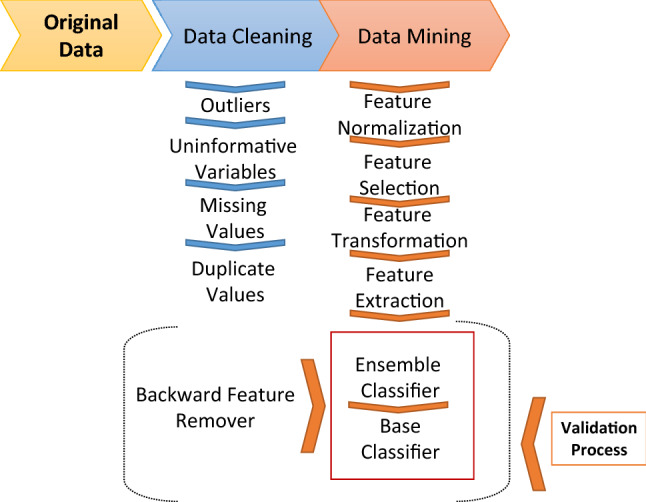
Biomarker data mining analyses procedure. First, a Data Cleaning process was performed to eliminate outliers, uninformative variables, missing values, and duplicate variables. Next, this new cleaned data set was used to train the model of the Data Mining process which is subdivided in different mathematical sub-processes: Feature Normalization, Feature Selection, Feature Transformation, Feature Extraction, Ensemble Classifier, Base Classifier, Backward Feature Removal and Validation. The Feature Normalization guarantees that the values of all variables are in the same range. The Feature Selection is applied to select the input variables that show the strongest relationship with the outcome. The Feature Transformation consists in mathematical transformations of the input data required for the Base Classifiers. It was not necessary to apply a Feature Extraction to reduce the number of random variables. Different algorithms generated different Base Classifiers with a good performance. Ensemble Classifiers were able to improve the performance of the Base Classifiers. Finally, the Validation process to estimate the accuracy of the predictive model was performed using the original database by several methods: 10-K fold and Leave-one-out.

Figure 2.

Representation of different possible models resulting from the data mining analysis in the whole cohort. (A) Sampling distribution graph representing the distribution of CR and NR patients for E-cadherin expression. When the classifier contains only one variable we used a variable brute force technique. The discriminant function is a constant that is determined as the threshold value that separates samples from the two groups with the best accuracy (marked by dotted red line). (B) Sampling distribution graph in 2D representing the distribution of CR and NR patients for the expression of AIP and E-cadherin. The blue line is the mathematical function defined by the values of the classifier, a mathematical function that separates NR from CR patients. As this classifier is composed of two variables, each dimension of the graph stands for one variable. The variables were selected by the Lasso method and the model performed according to Multilayer perceptron (MLP) methodology. (C) Sampling distribution graph in 2D representing the distribution of CR and NR patients for the expression of SSTR2, E-cadherin and AIP. As this classifier is composed of more than two variables, each dimension of the grafh stands for the the two main components after performing a principal component analysis (PCA). The blue line is the mathematical funtion that separates CR from NR patients. The variables were selected by the Wilcoxon method and the model performed according to Multilayer perceptron (MLP) methodology.

Feature Transformation, Feature Extraction, Ensemble Classifier, Base Classifier, Backward Feature Removal and Validation (Fig. 1). By means of artificial intelligence (AI) procedures, different mathematical algorithm approaches previously published were explored for each sub-process, allowing an exhaustive exploitation of the data (Table 1). In the present study the Feature Normalization determined that the values of all the variables were in the adequate range for the analysis, thus no further method of normalization was required. It was not necessary to apply a Feature Extraction to reduce the number of random variables. Different algorithms generated different classifiers. Since our goal was the prediction of SRL response for an individual case, we wanted to estimate how accurately a predictive model would perform in clinical practice. In order to flag selection bias or overfitting in our models, we used cross-validation techniques for assessing how the model would generalize to an independent data set. We confronted the model obtained with a subset of training data with the test data using a 10-K fold strategy. Therefore, we obtain a more exact estimation of the accuracy of the model taking the average of all the accuracy estimations obtained after each iteration. We used the accuracy (ACC) as the simplest parameter for evaluating the model, being the proportion of correct predictions (both true positives and true negatives) among the total number of samples. Accuracy levels are referred in these terms: accuracy 100–95%, excellent; 95%-80%, very good; 80%-70%, good; below 70%, to be improved.

Table 1.

Mathematical methods explored during the different processes included in the Data Mining strategy.

Sub-process	Algorithm	References
Backward removal features	Backward elimination	27
Base classifier	Elastic net	28
	K-nearest neighbors (K-NN)	29
	Boosted Generalized Additive Models (B-GAM)	30
	Tree	31
	Support vector machine (SVM)	32
	Multilayer perceptron (MLP)	33
	MLP ensemble	33
	Linear search	21
	Linear regression	21
	Quadratic	21
	Random linear	21
	Generalized linear model binomial	22
	Ridge regression	34
	Naïve bayes	35
	Lasso regression	36
	Radial basis function (RBF)	37
Cost function	Accuracy	38
	Balanced accuracy	38
	Balanced cost matrix	38
	Cost matrix	38
	F1 score	38
	Matthews correlation coefficient (MCC)	39
	Area Under Curve (AUC)	40
Dimensionality reduction	Principal component analysis (PCA)	41
	T-distributed Stochastic Neighbor Embedding (t-SNE)	42
	Multidimensional scaling (MDS)	43
	Hessian locally linear embedding (HLLE)	44
	Isomap	45
	Latent Dirichlet allocation (LDA)	46
	Locally linear embedding (LLE)	47
	Sammon projection	48
	LandMark ISOMAP (L-ISOMAP)	49
	Laplacian	50
	Gaussian process latent variable model (GPLVM)	51
	Kernel PCA	52
	Independent component analysis (ICA)	53
	Non-negative matrix factorization (NMF)	54
	Factor analysis	55
	Probabilistic principal component analysis (PPCA)	56
	Local tangent space alignment (LTSA)	57
Ensemble classifier	Bootstrap	58
	Bootstrap respecting prevalence	58
	Balanced bootstrap	58
Ensemble method	Bootstrap	59
	Bootstrap respecting prevalence	59
	Balanced bootstrap	59
Feature selection	K-nearest neighbors (K-NN)	29
	Receiver operating characteristic (ROC)	60
	Bhattacharyya	61
	Ridge regression	61
	Wilcoxon	62
	Wilcoxon + correlation	62
	minimum Redundancy Maximum Relevance (mRMR) Mean discretized	63
	Boolean balanced three-valued logic rules	64
	Sequential floating forward selection (SFFS)	65
	Support vector machines recursive feature elimination (SVM-RFE)	66
	Random forest	67
	Chow-Liu	68
	Simple regression	21
	Relieff	69
	Random generalized linear model	22
	One variable brute force	70
	Bhattacharyya + Correlation	71
	Entropy	71
	Entropy + Correlation	71
	Mattest	71
	T-test	71
	T-test + Correlation	71
	minimum Redundancy Maximum Relevance (mRMR)	72
	Lasso	36
	Elastic net	73
	Double Cross-Validation regression	74
Feature transformation	Sigmoid	71
	Gaussian: the value used is the value obtained after being submitted to a Gaussian function
	No value transformation
	The value used is the original value multiplied by itself
	The value used is the square root of the original value
Multiclass classifier	Generalized coding	71
	One versus all (OVA) binary classified applied
	One versus one (OVO) binary classifiers applied
Normalization	Sigmoidal mean variance	71
	Trimmed mean variance	71
	Mean variance
	Median dispersion
	Min Max: each value is divided by the difference between the maximum and the minimum value
	Winsorizing mean variance
Validation	Bootstrap	75
	K-Fold	76
	LeaveOneOut (LOO)	71

Results

Phenotypical characterization according to first-generation SRL response

A phenotypical characterization was performed according to SRL response which showed that SRL resistance was strongly associated with tumor extrasellar extension (Pearson χ² p‐value: 0.004) as shown in Table 2. Furthermore, NR patients presented more sinus invasion and hypopituitarism before surgery in contrast to CR or PR (Pearson χ² p‐value: 0.05 and 0.01, respectively). However, it is debatable whether the association of hypopituitarism is of clinical significance since we would have expected a progressive behavior from CR to NR, thus with a potential association of NR with hypopituitarism which may have been related with a larger and more destructive adenoma rather than a marked difference in the PR group.

Table 2.

Clinical categorical variables related to SRL response.

	Group	SRL responsea			Pearson χ2 p-valueb
		CR	PR	NR
Presurgical hypopituitarism	Yes	42%	15%	55%	0.01
	No	68%	85%	45%
Presurgical visual alterations	Yes	13%	27%	19%	0.62
	No	87%	73%	81%
T2 signal intensity	Hypointense	31%	22%	36%	0.90
	Isointense	38%	56%	36%
	Hyperintense	31%	22%	28%
T1 signal intensity	Hypointense	61%	40%	53%	0.75
	Isointense	39%	50%	38%
	Hyperintense	0%	10%	8%
Gender	Male	46%	35%	62%	0.07
	Female	54%	65%	38%
GNAS mutation	Mutated	29%	38%	36%	0.83
	WT	71%	62%	64%
Sinus Invasion	Yes	22%	35%	59%	0.05
	No	78%	65%	41%
Extrasellar growth	Yes	48%	60%	95%	0.004
	No	52%	40%	5%

^aSRL response columns indicate the percentage of patients with CR, PR, or NR dictated by the presence of absence of the clinical condition.

^bPearson χ2 p-values are shown. Statistically significant values (p-value < 0.05) are reported in bold.

Additionally, differences in the value of quantitative clinical variables according to SRL response categories were evaluated for the studied comparisons and the results are displayed in Table 3. High BMI and IGF1 levels at diagnosis were associated with NR patients.

Table 3.

Clinical numerical variables showing differences between the evaluated comparisons.

Variable	CR + PR vs NR		CR vs NR		PR vs NR		CR vs PR
	p-value	Log2FC	p-value	Log2FC	p-value	Log2FC	p-value	Log2FC
IGF1 diagnosis	0.035	− 0.33	0.007	− 0.47	0.722	− 0.16	0.081	− 0.31
IGF1 index diagnosis	0.051	− 0.41	0.086	− 0.39	0.063	− 0.43	0.838	0.04
GH diagnosis	0.590	1.04	0.134	0.94	0.429	1.17	0.134	− 0.22
GH after OGTT	0.622	1.27	0.728	1.29	0.633	1.25	0.941	0.03
BMI diagnosis	0.094	− 0.13	0.044	− 0.17	0.452	− 0.07	0.316	− 0.10
Maximum diameter	0.178	− 0.27	0.092	− 0.35	0.532	− 0.16	0.708	− 0.19
Age diagnosis	0.197	0.14	0.272	0.13	0.802	− 0.03	0.276	0.16

The clinical numerical variables that were tested: IGF1 levels measured at diagnosis in each center, IGF1 index at diagnosis, GH levels measured at diagnosis in each center, GH levels measured after a 75 g oral glucose load (OGTT), BMI (Body Mass Index) at diagnosis, maximum tumor diameter in the MRI measured in each center and the age of the patient at diagnosis. T-test or Wilcoxon-test p-values are shown. Statistically significant values (p-value < 0.05) are reported in bold, and p-value < 0.1 in italic Log2FC: Log2 Fold Change.

Algorithms classifying SRL response in acromegaly patients

The in-depth statistical exploration of the data generated in our previous paper¹¹ allowed to formulate several algorithms for the discrimination of patients regarding SRL response (cross‐validated p‐value < 0.05); those displaying the highest accuracy are shown in Table 4. All the significant predictive models are presented in Supplementary Tables. The strongest and most accurate single predictive biomarker for SRL response was E-cadherin, as it was the only marker discriminating between 3 of the 4 comparisons categories evaluated: (1) CR vs PR accuracy 65.8% at cut-off values of 0.513 and 0.007; (2) CR vs NR accuracy 73.1% at cut-off value 0.535; (3) CR + PR vs NR accuracy 62.6% at cut-off values of 0.348 and 0.013. Moreover, E-cadherin was also found in many of the dual and triad panels obtained by the analysis. After E-cadherin, the most frequent contributor to enhance classification power was SSTR2. The combination of E-cadherin and SSTR2 increased the accuracy by 6–7% more than E-cadherin alone. The addition of AIP⁷⁷ or In1-GHRL⁷⁸ showed a moderate enhancement of the classification power, reaching 75% of accuracy. Finally, adding PEBP⁷⁹ displayed nearly a 70% accuracy at cut-off 15.56, specifically in the discrimination between CR and PR.

Table 4.

Best classifiers in the whole cohort.

Evaluated comparison	Panel of classifiers	ACC	p-value
CR + PR vs NR	E-cadherin	62.61%	0.027
	GHRL	67.26%	0.002
	SSTR2 + E-cadherin	69.95%	0.001
CR vs NR	DRD2 long isoform	69.23%	0.006
	E-cadherin	73.08%	0.001
	SSTR2 + E-cadherin + AIP	75.00%	< 0.001
	SSTR2 + E-cadherin + IN1GHRL	75.00%	< 0.001
PR vs NR	SSTR2 + Ki-67	67.87%	0.02
	SSTR2 + SSTR5 + ARRB1	69.68%	0.004
CR vs PR	E-cadherin	65.84%	0.028
	PEBP1	69.68%	0.004

All individual classifiers and those panels with 2 or 3 classifiers that display an improvement in accuracy are presented in this table. ACC: Accuracy.

For those panels including more than one marker, in pairs or triads, cut-off values showed dynamic values (the values change with respect the variables of the model as a function because the variables are interdependent) as shown in Fig. 2B,C.

Fragmented population analysis achieves higher predictive accuracy

For analysis purposes, the cohort was subsequently segregated according to different clinical and biological variables, such as sex, extrasellar growth of the tumor, radiological sinus invasion, the mutational status of GNAS, T2 hypointense signal⁸⁰ and presurgical SRL treatment. The fragmented population studied is detailed in Supplementary Table 1.

The analysis provided multiple models depending on the core variable used in the fragmentation. The best models for every clinical scenario are shown in Table 5. Overall, the algorithms generated achieved a much higher cross‐validated accuracy in the fragmented rather than in the whole cohort for prediction of SRL response, as detailed in Supplementary Tables.

Table 5.

Best classifiers in patients with or without SRL presurgical treatment, extrasellar growth, sinus invasion, biological sex and GNAS mutational status.

Fragmenting condition	Evaluated comparison	Fragmented population Na	Best panel of classifiers	ACC	p-value
A. SRL presurgical treatement	CR + PR vs NR	No (9 vs 7)	PLAGL1 + PEBP1 + E-cadherin	88.89%	0.003
		Yes (33 vs 19)	SSTR5 + DRD2 long isoform + E-cadherin	70.65%	0.001
	CR vs NR	No (6 vs 7)	Age + SSTR2 + E-cadherin	100.00%	5.83E−04
		Yes (20 vs 19)	PLAGL1 + IN1GHRL + E-cadherin	76.97%	9.43E−04
	PR vs NR	No (3 vs 7)	Not found	–	–
		Yes (13 vs 19)	SSTR5 + PEBP1	74.29%	0.003
	CR vs PR	No (6 vs 3)	SSTR2 + E-cadherin	100%	0.012
		Yes (20 vs 13)	PEBP1 + IN1GHRL	76.82%	4.02E−04
B. Extrasellar growth	CR + PR vs NR	No (18 vs 1)	Not found	–	–
		Yes (20 vs 19)	GHRL	71.32%	0.005
	CR vs NR	No (12 vs 1)	Not found	–	–
		Yes (11 vs 19)	Not found	–	–
	PR vs NR	No (6 vs 1)	Not found	–	–
		Yes (9 vs 19)	Not found	–	–
	CR vs PR	No (12 vs 6)	SSTR5 + PEBP1	87.50%	0.004
		Yes (11 vs 9)	SSTR5 + IN1GHRL + E-cadherin	79.80%	0.012
C. Sinus Invasion	CR + PR vs NR	No (26 vs 7)	Not found	–	–
		Yes (12 vs 10)	AIP	77.50%	0.015
	CR vs NR	No (18 vs 7)	SSTR2 + ARRB1 + KLK10	81.75%	0.007
		Yes (5 vs 10)	PEBP1 + AIP + IN1GHRL	85.00%	0.017
	PR vs NR	No (8 vs 7)	Ki-67 + IN1GHRL	85.71%	0.007
		Yes (7 vs 10)	Not found	–	–
	CR vs PR	No (18 vs 8)	SSTR2 + IN1GHRL + KLK10	86.61%	0.009
		Yes (5 vs 7)	Not found	–	–
D. Gender	CR + PR vs NR	Female (25 vs 10)	PEBP1 + GHRL	73.78%	0.007
		Male (18 vs 16)	Age + E-cadherin	80.83%	0.001
	CR vs NR	Female (14 vs 10)	PEBP1 + E-cadherin + AIP	79.76%	0.005
		Male (12 vs 16)	Age + PLAGL1 + E-cadherin	85.45%	4.91E−04
	PR vs NR	Female (11 vs 10)	Not found	–	–
		Male (6 vs 16)	SSTR2 + PLAGL1 + GHRL/ARRB1	85.35%	0.003
	CR vs PR	Female (14 vs 11)	SSTR2 + PEBP1	74.68%	0.016
		Male (12 vs 6)	DRD2 short and long isoform + E-cadherin	80.00%	0.018
E. GNAS mutational status	CR + PR vs NR	WT (19 vs 14)	SSTR2 + DRD2 long isoform + ARRB1	77.07%	0.003
		Mutated (10 vs 5)	Not found	–	–
	CR vs NR	WT (10 vs 14)	Not found	–	–
		Mutated (5 vs 5)	PLAGL1 + E-cadherin + Ki-67	90.00%	0.024
	PR vs NR	WT (9 vs 14)	SSTR5 + ARRB1	72.22%	0.014
		Mutated (5 vs 5)	Not found	–	–
	CR vs PR	WT (10 vs 9)	PEBP1 + E-cadherin	84.44%	0.004
		Mutated (5 vs 5)	Not found	–	–
F. Hypointense T2 signaling	CR + PR vs NR	NO HYPO (23 vs 15)	SSTR3 + ARRB1 + AIP	74.18%	0.008
		HYPO (14 vs 8)	DRD2 short isoform + Ki-67	75.00%	0.040
	CR vs NR	NO HYPO (13 vs 15)	SSTR3 + SSTR2 + Ki-67	88.46%	8,75E−05
		HYPO (9 vs 8)	E-cadherin	87.50%	0.003
	PR vs NR	NO HYPO (10 vs 15)	Age + DRD2 short isoform + PEBP1	76.79%	0.022
		HYPO (5 vs 8)	Not found	–	–
	CR vs PR	NO HYPO (10 vs 9)	DRD2 short isoform + KLK10	85.04%	0.001
		HYPO (5 vs 5)	Not found	–	–

For each subgroup, the best panel/s of classifiers (with accuracy higher than the maximal one achieved by the classifiers using the whole cohort without fragmentation) in each comparison are shown. ^aThe third column refers to the condition in the first column. ACC Accuracy.

Decision tree therapeutic algorithms based on mathematical modelling

The present analyses allow the development of decision trees that may be used in clinical practice for individual patients. Two trees were formulated. The first one is based on the extrasellar tumor growth and different molecular biomarkers (Fig. 3A). A patient without extrasellar growth is discarded as NR with an accuracy of 95%, and for distinction between CR and PR, the measurement of PEBP1 and SSTR5 allows to achieve an accuracy of 87.5%. When tumor extrasellar growth is present, the decision tree segregates NR patients from responders (CR and PR) using levels of GHRL expression with an accuracy of 71.3%. To differentiate between CR and PR, measurement of SSTR5, In1-GHRL and E-cadherin leads to an accuracy of 79.8%. A second tree based on the patient’s sex showed an accuracy of 73.8–80.8% to distinguish between NR, CR and PR patients, being higher for men than for women (Fig. 3B).

Figure 3.

Best therapeutic tree decision algorithms based on mathematical modelling. (A) Decision tree to determine the first line drug for a given acromegaly patient based on the extrasellar tumor growth and molecular information. A patient without extrasellar growth is automatically classified as CR/PR without performing any molecular analysis (NR category is discarded with an accuracy of 95%). Then, by measuring the gene expression of SSTR5 and PEBP1 a clinician would be able to assign the right treatment with an accuracy of 87.5%. If the tumor has extrasellar growth, the gene expression of GHRL should be measured. If levels are < 0.008 or > 0.04, the patient is classified as NR with an accuracy of 71.3%, while if levels are between 0.008 and 0.04, the patient is classified as CR/PR. Then, by measuring the gene expression of SSTR5, IN1GHRL and E-cadherin a clinician would be able to assign the right treatment with an accuracy of 79.8%. When classifiers are composed of more than one variable (e.g. SSTR5 and PEBP1 or SSTR5, IN1GHRL and E-cadherin), the distribution of CR and PR patients is defined by a mathematical function (the blue line in the scatterplots) that separates CR from PR patients (blue and pink dots in the scatter plots, respectively). The details of the scatter plots and the mathematical models can be found in the Supplementary Figures S1-S3. (B) Decision tree exploiting molecular differences according to sex to accurately treat an acromegaly patient. If the patient is a male, the expression of E-cadherin should be measured and together with age it would be able to classify the patient as NR with an accuracy of 80.8%. If it is classified as CR/PR, the expression of the short and long DRD2 isoforms should be analyzed and together with E-cadherin it would be able to assign the right treatment with an accuracy of 80.0%. If the patient is a female, the expression of PEBP1 and GHRL should be measured and this will allow to classify the patient as NR with an accuracy of 73.8%. If it is classified as CR/PR, the expression of the short and long DRD2 isoform should be analyzed and together with E-cadherin it would allow to assign the right treatment with an accuracy of 74.7%. The details of the scatter plots and the mathematical models can be found in the Supplementary Figures S4-S7. ACC Accuracy, CR complete responder, PR partial responder, NR non-responder.

Both algorithms show a high accuracy to identify NR patients (accuracy ranging from 71.3 to 95%) which is particularly important since NR are the patients that suffer the largest delay using the current fixed sequential therapeutic decision chart. In all cases, measuring the expression of one or two molecules would be enough to define this type of patient response. The accuracy to distinguish between CR and PR patients is lower except for patients without extrasellar growth, thus we recommend the use of these algorithms specially to identify NR patients. When models are combined, the accuracies of the different steps should be multiplied to obtain the total final accuracy. Detailed mathematical features of the models can be found in Supplementary Figures S1-7.

Discussion

General findings in our cohort included a substantial association between first-generation SRL response and invasive tumors. BMI and IGF1 basal levels were also slightly associated with SRL response. Although high BMI used to be associated with acromegaly condition⁸¹, it is the first time that this association has been also identified regarding SRL response. Also, molecular differences match with the sexual dimorphism of SRL response⁸². In particular, PEBP1 was associated with the prediction of SRL response in women more than in men, as previously reported⁷⁹. Moreover, age, which has also been considered as a SRL response factor⁸³, seems to be more important in men. Furthermore, as we firstly¹¹ reported, the hypointense T2 MRI signal was associated with a better SRL response, also confirmed by others⁸⁴. In our cohort, non T2-hypointense tumors showed less heterogeneity allowing a better classification by AI procedures. Interestingly, SSTR3 contributed to classify the T2-hypointense tumors while it was not associated with any other clinical feature.

Nonetheless, single markers are not powerful enough to achieve a highly accurate and discriminative capacity of first-generation SRL response categorization in such heterogeneous disease as acromegaly. Our data definitely confirm that E-cadherin is one of the most powerful markers of SRL response prediction, as initially described by Fougner et al.⁸⁵. In our analysis SSTR2, although being a cardinal biomarker for developing a predictive algorithm, was insufficient as a single marker tool of SRL response prediction. The variability in the ability of SSTR2 to predict SRL response has been reported in different studies. Some authors found no statistical differences between SSTR2 and SRL response¹⁹ while others did^86,87. Wildemberg et al. assessed the performance of SSTR2 as a marker of SRL response and found a sensitivity of 100% and specificity of 38%⁸⁸, which represent a better sensitivity but a worse specificity compared to what we previously found (60% and 75%, respectively)¹¹. These differences may be due to the use of different methodologies to quantify SSTR2, to the criteria applied to categorize patient’s response or to biological differences between the cohorts, as these tumors are highly heterogeneous.

Most of the molecules that previously emerged from classical candidate gene approach as potential biomarkers of response to SRL are fairly represented in the algorithms and decision trees obtained in our analyses using data mining. Thus, from the different molecules previously reported as single markers: E-cadherin, SSTR2, PEBP1, GHRL and In-1-GHRL, and AIP are those that contribute -with different combinations at individual level- more robustly to the generation of decision trees and models in our cohort. Regarding AIP, although mutations in that gene are the most frequent germline mutations in somatotropinomas⁸⁹ and are associated with poorly response to first generation SRL response, our cohort did not include any AIP-mutated case. Instead, we analyzed AIP expression since AIP levels have been also related to SRL resistance^90,91.

To date, the best single marker is just able to predict with an accuracy not higher than 70%. In our study we were able to obtain accuracies that were above 70% and in some cases were ranging from 80 to 100% depending on the algorithm, thus one of the conclusions of our work is that in the future, acromegaly patients with specific characteristics will probably require specific decision trees obtained from enriched large cohorts. In this regard the present study is a preliminary work with internal validation procedures but awaiting of external validation with other similar cohorts.

The other very important issue is the definition of the cut-off values for application to clinical practice; in the present study we have been able to define cut-off values for the different clinical scenarios which may be useful for clinical implementation. The cut-off values obtained are not precise numbers applicable to all patients but instead they are dynamic, interdependable values calculated from the formulated equations (the mathematical models) that change for every single patient according to his or her clinical characteristics and/or to the expression of the markers in the tumor. The mathematical models we present, once established, will be easy to use, provided that the necessary biological markers will be determined in the tumor tissue. This kind of model is already used in other medical specialties, such as oncology. We strongly believe that acromegaly is a disease that will benefit enormously from this type of model decision algorithm. First, because there is an increasing number of therapies available; so, the “trial and error” approach would be unethical and impractical in the near future. Secondly, although acromegaly is a chronic disease and usually not acutely life-threatening, modern medicine is focused on quality of life which is heavily impaired in acromegaly and achieving a fast biochemical control could improve it considerably. Moreover, patient-reported outcomes (PRO) are increasingly been considered as the gold standard and included in guidelines and decisions by policy makers. In this regard, to have the option of choosing the most appropriate treatment for a given patient is the aim of contemporary medicine.

The present study has some limitations, being the most important the relatively low number of cases, but our results provide a proof-of-concept for the use of data mining strategies in the management of acromegaly patients. Thus, a constraint for implementation of personalized medicine, whether derived from classic or novel methods, is the necessity of validation of the proposed algorithms with other cohorts. However, by using data mining, the intrinsic nature of the mathematical analysis performs a continuous internal validation process; despite this, an external validation by an international consortium, capable of establishing a large cohort of acromegaly patients would be essential, since a substantial bias remains when this methodology is applied to small data sets⁹². Nonetheless, a study performed in a Brazilian cohort found models with a very similar performance⁹³. The mathematical modelling was very similar in both studies but the data used to construct the models were very different. The Brazilian cohort was larger, consisting of 153 patients in total, and the models were generated using demographic data (age and sex), biochemical data (GH and IGF1 levels at diagnosis and before SRL treatment) and immunohistochemical data (granulation pattern and immunoreactivity score of SSTR2 and SSTR5), but they did not include MRI information. On the other hand, while we used RT-qPCR to quantify the molecular biomarkers, they used immunohistochemistry, a more widely used technique easily found in most hospitals but whose results are particularly operator-dependent. Another difference lies in the categorization of SRL response. In the Brazilian study, they divided SRL response in two categories: CR and patients that do not achieve biochemical control with SRL (corresponding to the PR + NR patients of our classification). So, the aim of Wildemberg et al. was to identify CR, whereas our main goal was to discriminate NR from patients for those who SRL could be useful. In any case, the models from both studies still have some space of improving their performance in order to achieve accuracy at 95% level. Thus, the inclusion of other biomarkers not yet identified may certainly improve final obtained accuracy warranting further discovery investigation using omics approaches to complete all the molecular actors that may explain SRL response in an individual case at the molecular level. Finally, The use of RT-qPCR to measure the biomarkers may be a limitation since it requires specialized instruments not available in many centers; however, qPCR instrumentation and the use of qPCR-based tests are rapidly increasing in clinical laboratories, mainly because qPCR is a highly sensitive, specific and quantitative method, and it is a must in a specialized pituitary tertiary center as defined by the Pituitary Society⁹⁴.

In spite of the limitations, our preliminary results provide a proof-of-concept for the use of data mining strategies to generate improved mathematical algorithms that allow to apply personalized medicine and select the most suitable medical treatment for each acromegaly patient.

Author contributions

J.G.: conceptualization, coordination, administration, analysis, writing, review, figures. M.M.P.-project administration, review and clinical characterization of the patients. M.S., S.M.W., G.S., I.S., A.B., E.V., C.C., A.P., A.G.M., L.M.D., A.S.S., B.B., C.V., R.C., C.F.M., C.A.E., C.L., C.V.A., I.B. and M.M.: patient recruitment and review of final draft. T.S.: initial interpretations of results. M.J. and M.P.D.: project administration, review of all drafts and writing.

Funding

This work was funded by Instituto de Salud Carlos III (Grant no. PM 15/00027) and Novartis Farmacéutica (REMAH).

Data availability

The data that support the findings of this study are available on request from the corresponding authors. The data are not publicly available due to privacy and ethical restrictions.

Competing interests

MPD, MS, SMW, GS, IS, CFM, CL, EV, AP, CP, BB, CV, RC, CF, CVA, CAE, IB and, MM declare to have received funding from Novartis through the REMAH consortium for research purposes, and from Novartis, Ipsen and Pfizer as lecturers. TS was an employee of Anaxomics Biotech S.L. The other authors declared no conflicts of interest.

Supplementary Information

The online version contains supplementary material available at 10.1038/s41598-022-12955-2.

References

- 1.Melmed S. Medical progress: Acromegaly. N. Engl. J. Med. 2006;355:2558–2573. doi: 10.1056/NEJMra062453. [DOI] [PubMed] [Google Scholar]
- 2.Colao A, et al. Acromegaly. Nat. Rev. Dis. Prim. 2019;5:20. doi: 10.1038/s41572-019-0071-6. [DOI] [PubMed] [Google Scholar]
- 3.Gadelha MR, Wildemberg LE, Bronstein MD, Gatto F, Ferone D. Somatostatin receptor ligands in the treatment of acromegaly. Pituitary. 2017;20:100–108. doi: 10.1007/s11102-017-0791-0. [DOI] [PubMed] [Google Scholar]
- 4.Colao A, Auriemma RS, Pivonello R, Kasuki L, Gadelha MR. Interpreting biochemical control response rates with first-generation somatostatin analogues in acromegaly. Pituitary. 2016;19:235–247. doi: 10.1007/s11102-015-0684-z. [DOI] [PMC free article] [PubMed] [Google Scholar]
- 5.Colao A, Auriemma RS, Lombardi G, Pivonello R. Resistance to somatostatin analogs in acromegaly. Endocr. Rev. 2011;32:247–271. doi: 10.1210/er.2010-0002. [DOI] [PubMed] [Google Scholar]
- 6.Ritvonen E, et al. Mortality in acromegaly: A 20-year follow-up study. Endocr. Relat. Cancer. 2016;23:469–480. doi: 10.1530/ERC-16-0106. [DOI] [PubMed] [Google Scholar]
- 7.Geraedts VJ, et al. Predictors of quality of life in acromegaly: No consensus on biochemical parameters. Front. Endocrinol. 2017;8:2. doi: 10.3389/fendo.2017.00040. [DOI] [PMC free article] [PubMed] [Google Scholar]
- 8.Gadelha MR. A paradigm shift in the medical treatment of acromegaly: From a ‘trial and error’ to a personalized therapeutic decision-making process. Clin. Endocrinol. (Oxf) 2015;83:1–2. doi: 10.1111/cen.12797. [DOI] [PubMed] [Google Scholar]
- 9.Puig Domingo M. Treatment of acromegaly in the era of personalized and predictive medicine. Clin. Endocrinol. (Oxf) 2015;83:3–14. doi: 10.1111/cen.12731. [DOI] [PubMed] [Google Scholar]
- 10.Puig-Domingo M, et al. Pasireotide in the personalized treatment of acromegaly. Front. Endocrinol. 2021;12:2. doi: 10.3389/fendo.2021.648411. [DOI] [PMC free article] [PubMed] [Google Scholar]
- 11.Puig-Domingo M, et al. Molecular profiling for acromegaly treatment: A validation study. Endocr. Relat. Cancer. 2020 doi: 10.1530/ERC-18-0565. [DOI] [PubMed] [Google Scholar]
- 12.Gil J, et al. Molecular determinants of enhanced response to somatostatin receptor ligands after debulking in large GH producing adenomas. Clin. Endocrinol. 2020 doi: 10.1111/cen.14339. [DOI] [PubMed] [Google Scholar]
- 13.Cuevas-Ramos D, et al. A structural and functional acromegaly classification. J. Clin. Endocrinol. Metab. 2015;100:122–131. doi: 10.1210/jc.2014-2468. [DOI] [PMC free article] [PubMed] [Google Scholar]
- 14.Colao A, et al. Gender- and age-related differences in the endocrine parameters of acromegaly. J. Endocrinol. Invest. 2002;25:532–538. doi: 10.1007/BF03345496. [DOI] [PubMed] [Google Scholar]
- 15.Puig-Domingo M, et al. Magnetic resonance imaging as a predictor of response to somatostatin analogs in acromegaly after surgical failure. J. Clin. Endocrinol. Metab. 2010;95:4973–4978. doi: 10.1210/jc.2010-0573. [DOI] [PubMed] [Google Scholar]
- 16.Fougner SL, Casar-Borota O, Heck A, Berg JP, Bollerslev J. Adenoma granulation pattern correlates with clinical variables and effect of somatostatin analogue treatment in a large series of patients with acromegaly. Clin. Endocrinol. (Oxf) 2012;76:96–102. doi: 10.1111/j.1365-2265.2011.04163.x. [DOI] [PubMed] [Google Scholar]
- 17.Gil J, Jordà M, Soldevila B, Puig-Domingo M. Epithelial-mesenchymal transition in the resistance to somatostatin receptor ligands in acromegaly. Front. Endocrinol. 2021;12:2. doi: 10.3389/fendo.2021.646210. [DOI] [PMC free article] [PubMed] [Google Scholar]
- 18.Puig-Domingo M, et al. Molecular profiling for assistance to pharmacological treatment of acromegaly. Endocr. Abstr. 2018 doi: 10.1530/endoabs.56.OC13.3. [DOI] [Google Scholar]
- 19.Gonzalez B, et al. Cytoplasmic expression of SSTR2 and 5 by immunohistochemistry and by RT/PCR is not associated with the pharmacological response to octreotide. Endocrinol. y Nutr. 2014;61:523–530. doi: 10.1016/j.endonu.2014.05.006. [DOI] [PubMed] [Google Scholar]
- 20.Pedraza-Arévalo S, Gahete MD, Alors-Pérez E, Luque RM, Castaño JP. Multilayered heterogeneity as an intrinsic hallmark of neuroendocrine tumors. Rev. Endocr. Metab. Disord. 2018;19:179–192. doi: 10.1007/s11154-018-9465-0. [DOI] [PubMed] [Google Scholar]
- 21.Fukunaga K. Introduction to Statistical Pattern Recognition. Academic Press; 2013. [Google Scholar]
- 22.Madsen, H. & P.Thyregod. Introduction to General and Generalized Linear Models. Journal of Applied Statistics - J APPL STAT (2011).
- 23.Luque RM, et al. El Registro Molecular de Adenomas Hipofisarios (REMAH): una apuesta de futuro de la Endocrinología española por la medicina individualizada y la investigación traslacional. Endocrinol. y Nutr. 2016;63:274–284. doi: 10.1016/j.endonu.2016.03.001. [DOI] [PubMed] [Google Scholar]
- 24.Potorac I, et al. Pituitary MRI characteristics in 297 acromegaly patients based on T2-weighted sequences. Endocr. Relat. Cancer. 2015;22:169–177. doi: 10.1530/ERC-14-0305. [DOI] [PubMed] [Google Scholar]
- 25.Valls R, Pujol A, Artigas L, Mas JM. ANAXOMICS’ methodologies -Understanding the complexity of biological processes- White Pap. 2013;2:2. [Google Scholar]
- 26.Jorba G, et al. In-silico simulated prototype-patients using TPMS technology to study a potential adverse effect of sacubitril and valsartan. PLoS ONE. 2020;15:e0228926. doi: 10.1371/journal.pone.0228926. [DOI] [PMC free article] [PubMed] [Google Scholar]
- 27.Feature Extraction. vol. 207 (Springer, Berlin, 2006).
- 28.Gorban AN, Zinovyev A. Principal manifolds and graphs in practice: From molecular biology to dynamical systems. Int. J. Neural Syst. 2010;20:219–232. doi: 10.1142/S0129065710002383. [DOI] [PubMed] [Google Scholar]
- 29.Coomans D, Massart DL. Alternative k-nearest neighbour rules in supervised pattern recognition. Anal. Chim. Acta. 1982;136:15–27. doi: 10.1016/S0003-2670(01)95359-0. [DOI] [Google Scholar]
- 30.Wood SN. Fast stable direct fitting and smoothness selection for generalized additive models. J. R Stat. Soc. Ser. B Statistical Methodol. 2008;70:495–518. doi: 10.1111/j.1467-9868.2007.00646.x. [DOI] [Google Scholar]
- 31.Breiman L, Friedman J, Stone CJ, Olshen RA. Classification and Regression Trees. Chapman and Hall; 1984. [Google Scholar]
- 32.Cortes C, Vapnik V. Support-vector networks. Mach. Learn. 1995;20:273–297. [Google Scholar]
- 33.Haykin, S. O. Neural Networks and Learning Machines. (2008).
- 34.Ng, A. Y. Feature selection, L 1 vs. L 2 regularization, and rotational invariance. in Twenty-first international conference on Machine learning - ICML ’04 78 (ACM Press, 2004). doi:10.1145/1015330.1015435.
- 35.Russell S, Norvig P. Artificial Intelligence: A Modern Approach. Prentice Hall; 2010. [Google Scholar]
- 36.Tibshirani R. Regression shrinkage and selection via the lasso: a retrospective. J. R Stat. Soc. Ser. B Statistical Methodol. 2011;73:273–282. doi: 10.1111/j.1467-9868.2011.00771.x. [DOI] [Google Scholar]
- 37.Chang Y-W, Hsieh C-J, Chang K-W, Lin C-J, Ringgaard M. Training and testing low-degree polynomial data mappings via linear SVM. J. Mach. Learn. Res. 2010;11:1471–1490. [Google Scholar]
- 38.De Bièvre P. The 2012 international vocabulary of metrology: ``VIM’’. Accredit. Qual. Assur. 2012;17:231–232. doi: 10.1007/s00769-012-0885-3. [DOI] [Google Scholar]
- 39.Boughorbel S, Jarray F, El-Anbari M. Optimal classifier for imbalanced data using matthews correlation coefficient metric. PLoS ONE. 2017;12:e0177678. doi: 10.1371/journal.pone.0177678. [DOI] [PMC free article] [PubMed] [Google Scholar]
- 40.Fawcett T. An introduction to ROC analysis. Pattern Recognit. Lett. 2006;27:861–874. doi: 10.1016/j.patrec.2005.10.010. [DOI] [Google Scholar]
- 41.Pearson KLIII. On lines and planes of closest fit to systems of points in space. Dublin Philos. Mag. J. Sci. 1901;2:559–572. doi: 10.1080/14786440109462720. [DOI] [Google Scholar]
- 42.van der Laurens M, Geoffrey EH. Visualizing data using t-SNE. J. Mach. Learn. Res. 2008;164:10. [Google Scholar]
- 43.Borg I, Groenen PJF. Modern Multidimensional Scaling. Springer; 2005. [Google Scholar]
- 44.Donoho DL, Grimes C. Hessian eigenmaps: Locally linear embedding techniques for high-dimensional data. Proc. Natl. Acad. Sci. 2003;100:5591–5596. doi: 10.1073/pnas.1031596100. [DOI] [PMC free article] [PubMed] [Google Scholar]
- 45.Choi H, Choi S. Robust kernel Isomap. Pattern Recognit. 2007;40:853–862. doi: 10.1016/j.patcog.2006.04.025. [DOI] [Google Scholar]
- 46.McFarland HR, Richards DSP. Exact misclassification probabilities for plug-in normal quadratic discriminant functions. J. Multivar. Anal. 2002;82:299–330. doi: 10.1006/jmva.2001.2034. [DOI] [Google Scholar]
- 47.Wang J. Geometric Structure of High-Dimensional Data and Dimensionality Reduction. Springer; 2011. [Google Scholar]
- 48.Lerner B, Guterman H, Aladjem M, Dinsteint I, Romem Y. On pattern classification with Sammon’s nonlinear mapping an experimental study. Pattern Recognit. 1998;31:371–381. doi: 10.1016/S0031-3203(97)00064-2. [DOI] [Google Scholar]
- 49.Balasubramanian M. The isomap algorithm and topological stability. Science. 2002;295:7a–7. doi: 10.1126/science.295.5552.7a. [DOI] [PubMed] [Google Scholar]
- 50.Belkin M, Niyogi P. Laplacian eigenmaps for dimensionality reduction and data representation. Neural Comput. 2003;15:1373–1396. doi: 10.1162/089976603321780317. [DOI] [Google Scholar]
- 51.Li P, Chen S. A review on gaussian process latent variable models. CAAI Trans. Intell. Technol. 2016;1:366–376. doi: 10.1016/j.trit.2016.11.004. [DOI] [Google Scholar]
- 52.Schölkopf B, Smola A, Müller K-R. Nonlinear component analysis as a kernel eigenvalue problem. Neural Comput. 1998;10:1299–1319. doi: 10.1162/089976698300017467. [DOI] [Google Scholar]
- 53.Isomura T, Toyoizumi T. A local learning rule for independent component analysis. Sci. Rep. 2016;6:28073. doi: 10.1038/srep28073. [DOI] [PMC free article] [PubMed] [Google Scholar]
- 54.Tandon, R. & Sra, S. Sparse nonnegative matrix approximation: new formulations and algorithms. Tech. Rep. Max Planck Inst. Biol. Cybern.193, (2010).
- 55.Minka, T. P. Automatic Choice of Dimensionality for PCA. in Advances in Neural Information Processing Systems 13 (eds. Leen, T. K., Dietterich, T. G. & Tresp, V.) 598–604 (MIT Press, 2001).
- 56.Tipping ME, Bishop CM. Probabilistic principal component analysis. J. R Stat. Soc. Ser. B Statistical Methodol. 1999;61:611–622. doi: 10.1111/1467-9868.00196. [DOI] [Google Scholar]
- 57.Zhang Z, Zha H. Principal manifolds and nonlinear dimension reduction via local tangent space alignment. SIAM J. Sci. Comput. 2002;26:313–338. doi: 10.1137/S1064827502419154. [DOI] [Google Scholar]
- 58.Davison AC, Hinkley DV. Bootstrap Methods and Their Application. Cambridge University Press; 1997. [Google Scholar]
- 59.Efron B. Second thoughts on the bootstrap. Stat. Sci. 2003;18:135–140. doi: 10.1214/ss/1063994968. [DOI] [Google Scholar]
- 60.Wang, R. & Tang, K. Feature Selection for Maximizing the Area Under the ROC Curve. in 2009 IEEE International Conference on Data Mining Workshops 400–405 (IEEE, 2009). doi:10.1109/ICDMW.2009.25.
- 61.Xuan, G. et al. Feature Selection Based on the Bhattacharyya Distance. in Proceedings of the 18th International Conference on Pattern Recognition - Volume 03 1232–1235 (IEEE Computer Society, 2006). doi:10.1109/ICPR.2006.558.
- 62.Christin C, et al. A critical assessment of feature selection methods for biomarker discovery in clinical proteomics. Mol. Cell. Proteomics. 2013;12:263–276. doi: 10.1074/mcp.M112.022566. [DOI] [PMC free article] [PubMed] [Google Scholar]
- 63.Auffarth, B., Lopez, M. & Cerquides, J. Comparison of redundancy and relevance measures for feature selection in tissue classification of CT images. (2010).
- 64.Manning CD, Raghavan P, Schutze H. Introduction to Information Retrieval. Cambridge University Press; 2008. [Google Scholar]
- 65.Ververidis D, Kotropoulos C. Fast and accurate sequential floating forward feature selection with the Bayes classifier applied to speech emotion recognition. Signal Process. 2008;88:2956–2970. doi: 10.1016/j.sigpro.2008.07.001. [DOI] [Google Scholar]
- 66.Guyon I, Weston J, Barnhill S, Vapnik V. Gene selection for cancer classification using support vector machines. Mach. Learn. 2002;46:389–422. doi: 10.1023/A:1012487302797. [DOI] [Google Scholar]
- 67.Tin Kam Ho. Random decision forests. in Proceedings of 3rd International Conference on Document Analysis and Recognition vol. 1 278–282 (IEEE Comput. Soc. Press, 1995).
- 68.Chow C, Liu C. Approximating discrete probability distributions with dependence trees. IEEE Trans. Inf. Theory. 1968;14:462–467. doi: 10.1109/TIT.1968.1054142. [DOI] [Google Scholar]
- 69.Kira K, Rendell LA. Machine Learning Proceedings. Elsevier; 1992. A Practical Approach to Feature Selection; pp. 249–256. [Google Scholar]
- 70.Burnett M. Blocking Brute Force Attacks. University of Virginia UVA; 2007. [Google Scholar]
- 71.Pedregosa F, et al. Scikit-learn: Machine learning in python. J. Mach. Learn. Res. 2011;12:2825–2830. [Google Scholar]
- 72.Peng H, Long F, Ding C. Feature selection based on mutual information criteria of max-dependency, max-relevance, and min-redundancy. IEEE Trans. Pattern Anal. Mach. Intell. 2005;27:1226–1238. doi: 10.1109/TPAMI.2005.159. [DOI] [PubMed] [Google Scholar]
- 73.Zou H, Hastie T. Regularization and variable selection via the elastic net. J. R Stat. Soc. Ser. B Statistical Methodol. 2005;67:301–320. doi: 10.1111/j.1467-9868.2005.00503.x. [DOI] [Google Scholar]
- 74.Rodríguez-Girondo, M. et al. Sequential double cross-validation for assessment of added predictive ability in high-dimensional omic applications. (2016).
- 75.Efron, B. & Tibshirani, R. An Introduction to the Bootstrap. (1993).
- 76.Kohavi R. A Study of Cross-Validation and Bootstrap for Accuracy Estimation and Model Selection. Morgan Kaufmann; 1995. pp. 1137–1143. [Google Scholar]
- 77.Chahal HS, et al. Somatostatin analogs modulate AIP in somatotroph adenomas: The role of the ZAC1 pathway. J. Clin. Endocrinol. Metab. 2012;97:E1411–E1420. doi: 10.1210/jc.2012-1111. [DOI] [PubMed] [Google Scholar]
- 78.Ibáñez-Costa A, et al. In1-ghrelin splicing variant is overexpressed in pituitary adenomas and increases their aggressive features. Sci. Rep. 2015;5:8714. doi: 10.1038/srep08714. [DOI] [PMC free article] [PubMed] [Google Scholar]
- 79.Fougner SL, et al. Low levels of raf kinase inhibitory protein in growth hormone-secreting pituitary adenomas correlate with poor response to octreotide treatment. J. Clin. Endocrinol. Metab. 2008;93:1211–1216. doi: 10.1210/jc.2007-2272. [DOI] [PubMed] [Google Scholar]
- 80.Potorac I, Beckers A, Bonneville J-F. T2-weighted MRI signal intensity as a predictor of hormonal and tumoral responses to somatostatin receptor ligands in acromegaly: A perspective. Pituitary. 2017;20:116–120. doi: 10.1007/s11102-017-0788-8. [DOI] [PubMed] [Google Scholar]
- 81.Silverstein JM, et al. Use of electronic health records to characterize a rare disease in the U.S.: Treatment, comorbidities, and follow-up trends among patients with a confirmed diagnosis of acromegaly. Endocr. Pract. 2018;24:517–526. doi: 10.4158/EP-2017-0243. [DOI] [PubMed] [Google Scholar]
- 82.Eden Engstrom B, Burman P, Karlsson FA. Men with acromegaly need higher doses of octreotide than women. Clin. Endocrinol. 2002;56:73–77. doi: 10.1046/j.0300-0664.2001.01440.x. [DOI] [PubMed] [Google Scholar]
- 83.Suliman M, et al. Long-term treatment of acromegaly with the somatostatin analogue SR-lanreotide. J. Endocrinol. Invest. 1999;22:409–418. doi: 10.1007/BF03343583. [DOI] [PubMed] [Google Scholar]
- 84.Potorac I, et al. T2-weighted MRI signal predicts hormone and tumor responses to somatostatin analogs in acromegaly. Endocr. Relat. Cancer. 2016;23:871–881. doi: 10.1530/ERC-16-0356. [DOI] [PubMed] [Google Scholar]
- 85.Fougner SL, et al. The expression of E-cadherin in somatotroph pituitary adenomas is related to tumor size, invasiveness, and somatostatin analog response. J. Clin. Endocrinol. Metab. 2010;95:2334–2342. doi: 10.1210/jc.2009-2197. [DOI] [PubMed] [Google Scholar]
- 86.Casar-Borota O, et al. Expression of SSTR2a, but not of SSTRs 1, 3, or 5 in somatotroph adenomas assessed by monoclonal antibodies was reduced by octreotide and correlated with the acute and long-term effects of octreotide. J. Clin. Endocrinol. Metab. 2013;98:E1730–E1739. doi: 10.1210/jc.2013-2145. [DOI] [PubMed] [Google Scholar]
- 87.Casarini APM, et al. Acromegaly: Correlation between expression of somatostatin receptor subtypes and response to octreotide-lar treatment. Pituitary. 2009;12:297–303. doi: 10.1007/s11102-009-0175-1. [DOI] [PubMed] [Google Scholar]
- 88.Wildemberg LEA, et al. Low somatostatin receptor subtype 2, but not dopamine receptor subtype 2 expression predicts the lack of biochemical response of somatotropinomas to treatment with somatostatin analogs. J. Endocrinol. Invest. 2013;36:38–43. doi: 10.3275/8305. [DOI] [PubMed] [Google Scholar]
- 89.Bogusławska A, Korbonits M. Genetics of acromegaly and gigantism. J. Clin. Med. 2021;10:1377. doi: 10.3390/jcm10071377. [DOI] [PMC free article] [PubMed] [Google Scholar]
- 90.Ozkaya HM, et al. Germline mutations of aryl hydrocarbon receptor-interacting protein (AIP) gene and somatostatin receptor 1–5 and AIP immunostaining in patients with sporadic acromegaly with poor versus good response to somatostatin analogues. Pituitary. 2018;21:335–346. doi: 10.1007/s11102-018-0876-4. [DOI] [PubMed] [Google Scholar]
- 91.Kasuki L, et al. AIP expression in sporadic somatotropinomas is a predictor of the response to octreotide LAR therapy independent of SSTR2 expression. Endocr. Relat. Cancer. 2012;19:L25–L29. doi: 10.1530/ERC-12-0020. [DOI] [PubMed] [Google Scholar]
- 92.Vabalas A, Gowen E, Poliakoff E, Casson AJ. Machine learning algorithm validation with a limited sample size. PLoS ONE. 2019;14:e0224365. doi: 10.1371/journal.pone.0224365. [DOI] [PMC free article] [PubMed] [Google Scholar]
- 93.Wildemberg LE, et al. Machine learning-based prediction model for treatment of acromegaly with first-generation somatostatin receptor ligands. J. Clin. Endocrinol. Metab. 2021 doi: 10.1210/clinem/dgab125. [DOI] [PubMed] [Google Scholar]
- 94.Casanueva FF, et al. Criteria for the definition of pituitary tumor centers of excellence (PTCOE): A pituitary society statement. Pituitary. 2017;20:489–498. doi: 10.1007/s11102-017-0838-2. [DOI] [PMC free article] [PubMed] [Google Scholar]
Associated Data
This section collects any data citations, data availability statements, or supplementary materials included in this article.
Supplementary Materials
Data Availability Statement