Green two-echelon closed and open location-routing problem: application of NSGA-II and MOGWO metaheuristic approaches

Abstract

Nowadays organizations outsource transportation of goods or services to reduce cost which leads to a particular type of problem called open location-routing. Also, each logistic organization possesses a limited number of specific vehicles that may not be enough in certain circumstances. This issue indicates the importance of simultaneously considering both open and closed routs. On the other hand, the growing concerns about the detrimental environmental impacts of human activities reveal the necessity of paying attention to environmental issues in logistics. In this study, a bi-objective mathematical programming model is proposed for two-echelon close and open location-routing problem (2E-COLRP) including two echelons of factories, depots and customers to minimize costs and CO₂ emissions. The proposed model finds the optimal routs, optimal number of vehicles and facilities as well as the locations of facilities. The augmented epsilon constraint method is used as an exact method to solve the small-sized problems. Due to complexity of model, two metaheuristic algorithms named MOGWO and NSGA-II are utilized to tackle the problems. The efficiency of two aforementioned algorithms is evaluated in terms of several indices considering 22 problem instances with various sizes. The results show that MOGWO performs better than NSGA-II.

Introduction

Nowadays, supply chain networks that traditionally operate without considering environmental issues such as greenhouse gas emissions are not able to survive in these competitive markets (Diabat & Al-Salem, 2015). Hence, manufacturing industries must pay attention to these environmental issues in their supply chain. Supply chain management association defines supply chain management as follows: supply chain management involves the planning and management of supply chain activities, the conversion of goods from the raw material phase (extraction)to the end user, logistics activities and all coordination activities among suppliers, brokers, retailors and final users (Dawei et al., 2015).

According to the definition provided by Srivastava in 2007, green supply chain management is "the integration of environmental thinking in supply chain management including product design, material sourcing and selection, production processes, product delivery to consumers, and so on" (Srivastava, 2007).

One of the most important problems in the green supply chain design is the routing problem which aims to find the shortest path between origin and destination to reduce emissions effectively. Several optimization models have been provided to find the optimal locations for building facilities such as factory, distribution centers and paths among them (Soleimani et al., 2017).

Establishing new facilities (warehouses or depots) requires a great deal of investment and is expected to be used over a long period of time (Melo et al., 2009). The location of establishing these centers has a long-term impact on the overall performance of the supply chain and is one of the most important strategic decisions in the process of designing the supply chain network.

The vehicle routing problem (VRP) has numerous applications in real life. It clarifies in a wide area of transportation and distribution such as transportation of individuals and items, conveyance service and garbage collection. Thus, an appropriate selecting of vehicle routing has an extensive influence role to improve the economic interests and appropriateness of logistics planning (Mohammed et al., 2017). So, routing decision is a significant decision in addition to location and allocation decisions.

In LRP problem, decisions on the location of all types of facilities (example: factories, distribution centers, depots, hubs, transit warehouses) are merged with the decision-making problem on the route of the vehicles. It is well accepted that deciding on either of the above issues independently of the other can have a great impact on the optimal response (Salhi & Rand, 1989).

The two-echelon distribution systems are of the multi-echelon systems that are formed from three echelons, which have been considered in the last few years due to the applicability of these systems. The product flow from the origin to the destination is made at least through one or more of the intermediate facilities. Each category can be defined as a transportation interface between two adjacent surfaces. The level can be each type of facilities such as factory, warehouse, distribution centers or customers.

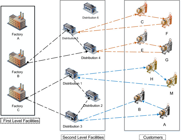
A distribution network consisting of three separate sets of principals that are, respectively, corresponding to: potential locations of factories (i.e., sources), potential locations of secondary facilities (i.e., intermediate echelon facilities or depots) and customers (i.e., destinations) is called a two-echelon distribution network. Customer location in this distribution network is predetermined and fixed. In other words, the location of the factories and the secondary facilities required in this type of distribution network are not predetermined (this is a general case and facilities of one of these echelons can be assumed fixed and adopt location decisions at least at one echelon). Figure 1 provides a general view of a 2E-LRP problem.

Fig. 1.

Two-echelon location-routing problem (LRP)

Outsourcing is one of the ways for decreasing the transportation costs in one or two levels of the distribution system. The open routing problem is defined corresponding with the situation in which the products cannot be returned to depot after delivery to customers. This condition happens when the company does not have enough vehicles or the capacity to supply the customers demand. Consequently, another transportation company is handled the problem under certain conditions (Repoussis et al., 2010). On the other hand, the detrimental effects of the transportation activities should be reduced. Environmental issues of the transportation sector are generally classified into four main categories including waste generation, energy usage, material recycling and the reduction of the greenhouse gas emissions (Soleimani et al., 2017). The VRP considering the reduction of carbon gas emissions in the transportation sector has been highly paid attention in recent years.

In this paper, a bi-objective optimization model for two-echelon routing problem consisting of three levels: factories, distribution center and customers is investigated. In this problem, we attempt to find a trade-off between the minimization of the total cost of the entire supply chain and the minimization of carbon dioxide emissions of the transportation sector in the first level (factory to the distribution center) as well as the second level (distribution center to customer). It should be noted that the distribution centers have to be located and the routing must be done in both levels. In addition, both possible scenarios including the availability of vehicles for supplying demand and lack or unavailability of vehicles are considered in the proposed mathematical programming model. In other words, the combination of closed routing (vehicles belonging to the company) and open routing (rented vehicles) is considered in this problem. The model is called two-echelon closed and open location-routing problem (2E-COLRP), which seeks to find the optimal location of distribution centers or depots, routes and transportation rates in both levels together with the optimal allocation of customers and depots.

The remainder of this paper is structured as follows. The related literature is briefly reviewed in Sect. 2. In Sect. 3, the problem is defined and the proposed mathematical programming model is presented. Section 4 explains the solution methods for the problem. In Sect. 5, model validation and sensitivity analysis are conducted. Finally, conclusions are expressed in Sect. 5.

Literature review

The relevant studies are presented in this section.

Two-echelon location-routing problem (2E-LRP)

In this particular type of LRP problem, first echelon routes are set up for transferring commodities from primary facilities to depots and created routes from established depots are also created to send goods to customers (second echelon) (Prodhon & Prins, 2014).

Among the earliest studies in the field of 2E-LRP, the paper by Jacobson et al. is considerable (Jacobsen & Madsen, 1980), in which the real problem of the newspaper distribution system in the western part of Denmark was examined.

Lin and Lei (2009) proposed a model for the 2E-LRP problem including two types of customers and a number of depots. They located the distribution centers and designed routes in two echelons. A genetic algorithm-based solving approach was also proposed for this model, in which results in small sizes were equal to the exact problem solving (Lin & Lei, 2009). Crainic et al. (2011) proposed a heuristic algorithm for solving the 2E-LRP problem assuming a facility at a zero-echelon and a limited -capacity facilities at one-echelon (Crainic et al., 2011). Nguyen et al. (2012) proposed a 2E-LRP model assuming a central depot and several candidate locations for other depots; in this model, the cost of establishing depots was different considering limited capacity (Nguyen et al., 2012). Martinez et al. (2014) proposed a bi-objective model for the 2E-LRP problem assuming multiple capacities at zero and one echelon and considering the fixed cost of establishing facilities at both echelons, direct transportation in first echelon and routing decisions with uniform fleet in second echelon. They applied two meta-heuristic methods to solve the model (Martínez-Salazar et al., 2014). Rahmani et al. (2016) proposed a MIP model for the 2E-LRP problem and used two meta-heuristic methods to tackle the problem (Rahmani et al., 2016). Vidović et al. (2016) presented a MIP model for the 2E-LRP in their paper to design a system for the collection and recycling of non-hazardous recyclable waste with a meta-heuristic method for its solution (Vidović et al., 2016). Zhao et al. (2018) applied a model for the 2E-LRP to the post sector with a heterogeneous transportation fleet and suggested a meta-heuristic method for solving the problem (Zhao et al., 2018). Pichka et al (2018) developed a model called two-echelon-open-location-routing-problem (2E-OLRP), assuming that vehicles do not return to depots. The researchers also used a meta-heuristic hybrid algorithm for their proposed model (Pichka et al., 2018). Darvish et al. (2019) developed a new type of 2E-LRP problem called the flexible locating-routing problem. Two types of flexibility were considered in this model: flexibility in delivery deadline and flexibility in designing distribution network. In order to solve this problem, an exact branch-and-bound method was proposed (Darvish et al., 2019). Amiri et al. (2019) presented a mixed integer nonlinear programming (MINLP) model of the 2E-LRP problem considering time windows and solved the problem with Lagrangian relaxation method (Amiri et al., 2019).

Abbassi et al. (2021) addressed the two-echelon location distribution problem for non-medical products and developed a multi-objective mathematical formulation considering the two objective functions of minimizing the total distribution cost and minimizing the total time of the distribution horizon. They used particle swarm optimization (PSO) and genetic algorithms to solve a real case of the distribution of non-medical products and then evaluated the efficiency and validation of the algorithms. Gao et al. (2020) investigated the two-echelon location-routing problem of biomass resources (2E-BRLRP). They developed a mixed integer programming model for the problem taking the predetermined supply of biomass resources into account to determine the best locations for biomass collection facilities and related vehicle routes. They also employed a hybrid heuristic algorithm for solving the problem using several computational examples. Fallahtafti et al. (2021) developed a two-echelon location-routing framework for cash transfer, in which a dynamic risk factor was considered to reduce the risk of theft in cash transfer. Then, they implemented exact and metaheuristic methods to solve the problem considering several small to medium examples. In addition, Gao and Institute (2020) reviewed the literature on two-echelon problems. In two-echelon mathematical models, as mentioned earlier, routing is considered in the first or second echelon or both. In this regard, Lu et al. (2019) assumed closed routing in both echelons. Rabbani et al. (2018) proposed a transportation-location-routing problem (TLRP) with the objective functions of reducing the distribution cost, fuel consumption, and carbon dioxide emissions along with balancing the workload for city drivers, taking the capacity of vehicles and the time window of customers into consideration. They exploited the NSGA-II and MOPSO algorithms to solve the problem and found out that MOPSO performed better for solving this problem. Ouhader and El kyal (2017) presented a two-echelon model taking the economic, environmental and social responsibility goals into account to deliver products from suppliers to customers and solved it using the epsilon constraint method.

Open-close vehicle routing problem

Open vehicle routing problem (OVRP) assumes that vehicles are not needed to go back to the central depot after visiting the final customer. If vehicles are to be returned, they must go back the opposite way and visit the same customers. In addition, the OVRP seeks to minimize two objectives including the total number of vehicles, and the whole distance (or duration) (Fleszar et al., 2009; MirHassani & Abolghasemi, 2011; Subramanian et al., 2013).

Liu and Jiang (2012) in their research proposed a new problem called closed–open-mixed-vehicle-routing-problem (COMVRP). The distinction of this model is to consider both the open and closed routes compared to the classic model of the vehicle routing problem. The researchers presented a MIP model and a meta- heuristic solution procedure for their problem (Liu & Jiang, 2012). One of the most recent research in this area by Vincent and Lin (2015) presented a heuristic algorithm based on simulated annealing heuristic (SA) to solve the problem of open vehicle routing. The computational results of applying this algorithm on four sets of standard problems indicate the high effectiveness of this method (Vincent & Lin, 2015). Rahmani Hosseinabadi et al. (2021) developed a meta-heuristic algorithm called OVRP_SAICA to solve OVRP. They compared the algorithm with several other algorithms and found that OVRP_SAICA performs better than all of them in solving the OVRP. Lalla-Ruiz and Mes (2021) proposed a two-index-based mathematical formulation for the MDOVRP. Also, they presented a memetic algorithm (MA) for solving the model. Sun et al. (2021) demonstrated the effectiveness of the heuristic-based initialization mechanism by a simulation experiment based on the 320 benchmark instances. Zhen et al. (2021) introduced a nonlinear mixed-integer programming model for OVRP that is a shared mobility based last mile delivery mode. Their proposed model was beneficial in terms of reducing the last mile delivery cost as well as advancing the modern transportation paradigm.

Ruiz y Ruiz et al. (2020) presented a method for improving the performance of OVRP. Their method is able to save the economic costs up to 20%. Yuchi et al. (2021) proposed a location-inventory-routing problem in a closed-loop supply chain (LIRP-CL). They also employed a novel hybrid heuristic algorithm based on tabu search (TS) and simulated annealing (SA). Purnawan et al. (2018) compared the results of two different algorithms, namely local solver (LS) algorithm and simulated annealing (SA) algorithm, for solving the gallon water closed-loop supply chain problem. Soto-Mendoza et al. (2020) presented a hybrid Grasshopper Optimization algorithm using a novel decoder to solve the OVRP. They conducted several experiments to minimize the total number of vehicles as well as the total distance. Ruiz et al. (2019) utilized a biased random-key genetic algorithm to solve the OVRP with capacity and distance constraints. Xia and Fu (2019) designed an OVRP with soft time windows and satisfaction rate to reduce the logistics distribution cost. They applied adaptive penalty mechanism, multi-neighborhood structure and re-initialization rule embedded in the Tabu Search (TS) algorithm, resulting in an improved TSA (ITSA). Atefi et al. (2018) addressed an OVRP with decoupling points (OVRP-DP); then, they applied a tailored iterated local search (ILS) algorithm to solve the problem. Rahmani (2021) developed a multi-cross-docking vehicle routing problem (MCVRP) which was a combination with close–open mixed VRP (COMVRP). Also, the problem was solved using the genetic algorithm (GA). Guo et al. (2018) proposed a location-inventory-routing problem for a closed loop supply chain. They also used the genetic algorithm (GA) to tackle the problem. Niu et al. (2018) presented a mathematical model for the green open vehicle routing problem considering time windows (GOVRPTW) and employed a hybrid Tabu Search (TS) algorithm to deal with the problem.

Routing problem considering pollutant emissions

Much of the greenhouse gas emissions and in particular carbon dioxide emissions are related to the road transportation sector. Emissions from these gases have direct and indirect harmful effects on humans and the entire ecosystem. This growing concern about the negative impacts of transportation on the environment necessitates the need to redesign the road transport network and the transient load flow, taking into account greenhouse gas emissions (Bektaş & Laporte, 2011).

Different approaches can be applied to the problem of vehicle routing in order to reduce emissions, including setting targets with the nature of environmental costs. The purpose of the PRP is to select a program for routs of vehicles with the lowest emissions and especially with the lowest carbon dioxide emissions. Studies in the area of PRP can be examined since 2007. By extending the goals of the classic VRP models and taking into account the social and environmental impacts of the transportation process, reducing carbon dioxide emissions is achievable (Bektaş & Laporte, 2011; Maden et al., 2010; McKinnon, 2007; Sbihi & Eglese, 2007).

Traditional VRP that aims to minimize the total travelled distance are also inherently aimed at reducing fuel consumption and minimizing the emission of environmental pollutants; however, this relationship must be measured directly by careful formulation. Pronello and Andre (2000) proposed models to measure the amount of pollution produced by vehicles. These models also included factors such as elapsed time with engine cooling conditions (Pronello & André, 2000). Sbihi and Eglese (2007) raised a TDVRP problem in the area of traffic control issues. In this case, when vehicles travel at optimum speed, they produce less pollution. In addition, distancing vehicles from the traffic congestion also reduces the harmful effects of the environment, although this will make the route longer (Sbihi & Eglese, 2007). In another study, Maden et al. (2010) developed a TDVRP model that, according to computational results, leads to 7% reduction in carbon dioxide emissions assuming different speeds of vehicles. However, the goal of the VRP model proposed by them was to minimize total costs rather than reduce emissions (Maden, et al., 2010). Bauer et al (2010) examined the impact of multi-state transportation systems on greenhouse gas emissions. They showed the potential impact of a multi-state transportation system on reducing emissions (Bauer et al., 2010). Fagerholt et al (2010) reduced fuel consumption and emissions by optimizing speed in a transportation scenario (Fagerholt et al., 2010). Kumar et al. (2016) proposed the multiple objectives optimization model for the PRP with considering both carbon generation and emission and solved it with two meta-heuristic approaches (Kumar et al., 2016). Navazi et al. (2021) proposed closed-loop location routing-inventory problem with three objectives of cost, environmental effects and social responsibilities. They applied the genetic algorithm (GA) to solve the large-sized problem. Dewi and Utama (2021) developed a hybrid whale optimization algorithm (HWOA) which is based on the whale optimization algorithm (WOA) combined with the Tabu Search (TS) algorithm and local search procedures to minimize the distribution cost of the green vehicle routing problem (GVRP) considering fuel consumption, carbon emissions and vehicle usage cost.

Liu et al. (2021) developed a sustainable location-routing-inventory model for the supply chain of perishable products considering costs, CO₂ emissions, and social responsibility (fresh and high-quality products for customer satisfaction). Babaee et al. (2020) proposed a location-routing model for hospital waste management to prevent the spread of Coronavirus. Masoudipour et al. (2020) developed a closed-loop supply chain model and solved it by the Lexicographic augmented ε-constraint method using CPLEX optimization software. Zandkarimkhani et al. (2020) presented a model for open-loop supply chain network design considering the location-routing problem. Biuki et al. (2020) presented a mathematical model for the location-routing-inventory problem of perishable products and exploited the GA and PSO metaheuristic algorithms to tackle the problem. Navazi et al. (2019) presented a sustainable location-routing model to collect expired products with forward and reverse routes. Zhang et al. (2018) developed a sustainable mathematical model for multi-depot location multi- routing problem in emergency situations considering the minimization of relief costs, travel time, and CO₂ emissions. They also used a genetic algorithm (GA) to solve the problem. Ebrahimi (2018) suggested a multi-objective random allocation-routing problem for the tire supply chain considering sustainability and discount. The objectives of minimizing costs and pollution were introduced as economic and environmental goals, respectively, and maximizing customer responsiveness was considered as social responsibility aspect, and the epsilon constraint method was used to solve the model.

The following table summarizes recent research works on VRP (Table 1).

Table 1.

The brief review of the relevant studies

Authors	Type of VRP		Method	Optimization goals
	Open	Closed		Economic	Social	Environmental	Time
Rahmani Hosseinabadi et al. (2021)	*		Meta-heuristic algorithm called OVRP_SAICA/C#.NET	*			*
Lalla-Ruiz and Mes (2021)	*		Two-index-based mathematical formulation /CPLEX	*
Sun et al. (2021)	*		MA/MATLAB	*
Yuchi et al. (2021)		*	Novel hybrid heuristic algorithm based on TSA and SA/Visual C++ 6.0 platform and an Intel(R)	*
Zhen et al. (2021)	*		Column generation-based solution method/CPLEX
Purnawan et al. (2018)		*	Local Solver algorithm and SA	*			*
Dewi and Utama (2021)	*		(WOA) combined (TSA)/MATLAB	*		*
Ruiz y Ruiz et al. (2020)	*		Cutting-plane method/CPLEX	*	*
Navazi et al. (2021)		*	TH method, GA/GAMS	*		*
Soto-Mendoza et al. (2020)	*		Hybrid Grasshopper Optimization Algorithm with Local Search/CPLEX	*
Guo et al. (2018)		*	GA/ MATLAB 2014a
Ruiz et al. (2019)	*		Biased random key GA/C++	*			*
Xia and Fu (2019)	*		(TSA)/ MATLAB	*
Rahmani (2021)		*	Robust optimization-GA/CPLEX	*
Atefi et al. (2018)	*		(ILS)/Visual Studio C++	*
Niu et al. (2018)			Hybrid (TSA)	*		*
Hamid Khan et al. (2021)		*	GA			*

As mentioned before, some organizations for reducing the cost of transportations outsource this unit of supply chain system. So, this subject leads to create a concept that is called open vehicle routing problem. In this study, both open and closed routs are used in routes in two-echelon location-routing problem.

The contributions of this study as compared to similar works can be stated as follows: considering both open and closed routes in two-echelon location-routing problem, Applying two objective functions aiming to minimize cost and CO₂ gas emissions in two-echelon closed and open location routing problem, Utilizing efficient meta-heuristic algorithms for solving the proposed problem.

Problem definition

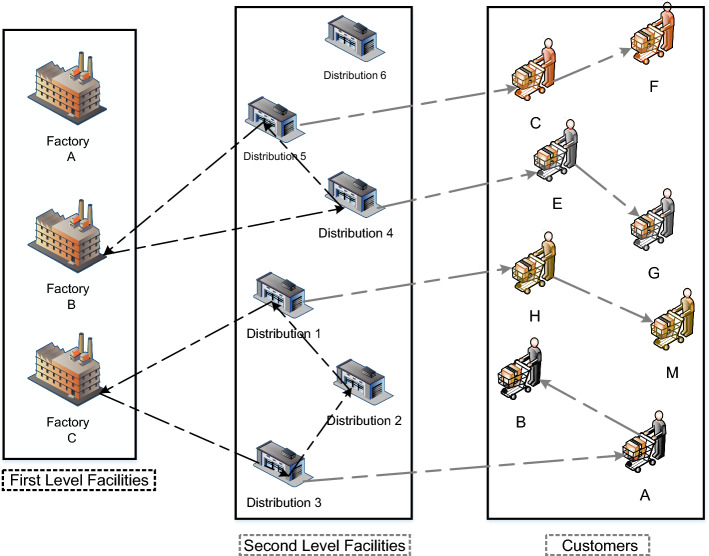
In this section, a bi-objective mixed-integer programming mathematical model is presented for two-echelon closed and open location-routing problem (2ECOLRP) by purpose of minimizing cost and CO2 gas emission throughout the supply network. Many researchers over the last few decades have established numerous researches and used many methods with different techniques to handle it. But, for all research, finding the lowest cost is very complex. However, they have managed to come up with approximate solutions that differ in efficiencies depending on the search space (Mohammed et al., 2017). In proposed model, the first echelon routes are closed and commence from a given factory, serve some depots and return to the first factory. However, the second echelon routes are open and begin from a given depot, serve some customers and do not go back to the first depot (Dai et al., 2019). Considering these assumptions for the proposed model, in addition to approaching the problem to real-world constraints, it will optimize the problem in terms of environmental impacts. A schematic of feasible solution of proposed problem is presented in Fig. 2.

Fig. 2.

A schematic of feasible solution of proposed problem

As can be seen in Fig. 2, the location decisions are performed only in second echelon, and all factories are pre-deployed on the first echelon and it is only the allocation decisions related to depots and customers, while the routing decisions should be adopted in both echelons.

The assumptions, indices, parameters and decision variables are presented as follows:

Assumptions, indices, parameters and decision variables of proposed model

1. Each customer demand is deterministic and known and each vehicle has a defined capacity.

2. Each depot must be served by one factory and one vehicle only.

3. The proposed model is single period and single product.

4. The number of vehicles is limited.

5. There are different types of vehicles that have different capacities and have different CO₂ gas emission coefficient in first echelon.

6. The production capacity of each factory and the storage capacity of each depot are limited

Let $G=(V,E)$ be a complete directed graph where $V=V_f\cup V_d\cup V_c$ denotes the set of all nodes of desired network. $V_f$, $V_d$ and $V_c$ indicate the factories in first echelon, the depots in second echelons and the customers in third echelons, respectively. And also, $E=\{\left(i,,,j\right):i,j\in V,i\ne j\}$ denotes the set of arcs between $i$ and $j$ and each arc has a distance equal to ${\mathrm{distance}}_{\mathit{ij}}$. Each of customer has a demand equal to $d_i$ that $0\le d_i\le {\mathit{CV}}_n$. The other indices, parameters and decision variables are presented in Table 2.

Table 2.

Indices, parameters and decision variables of proposed mathematical model

Sets $\mathit{V}$: set of all nodes $\mathit{V}={\mathit{V}}_{\mathit{f}}\cup {\mathit{V}}_{\mathit{d}}\cup {\mathit{V}}_{\mathit{c}}$ ${\mathit{V}}_{\mathit{f}}$: set of factories in first echelon ${\mathit{V}}_{\mathit{d}}$: set of facilities in second echelon (depots) ${\mathit{V}}_{\mathit{c}}$: set of customers in third echelon $\mathit{E}$: set of all arcs between nodes n: set of available vehicles in first echelon (factories)

Indices $\mathit{i}$, $\mathit{j}$, k: index for the nodes of all corresponding to all echelons n: index for the vehicles

Parameters ${\mathit{F}\mathit{C}\mathit{D}}_{\mathit{k}}$: the fixed cost of establishing intermediate facilities (depots) $\mathit{k}\in {\mathit{V}}_{\mathit{d}}$ ${\mathit{C}\mathit{F}}_{\mathit{k}}$: the capacity of factories $\mathit{k}\in {\mathit{V}}_{\mathit{p}}$ ${\mathit{C}\mathit{D}}_{\mathit{k}}$: the capacity of intermediate facilities (depots)$\mathit{k}\in {\mathit{V}}_{\mathit{d}}$ ${\mathit{d}}_{\mathit{i}}$: the demand of customers $\mathit{i}\in {\mathit{V}}_{\mathit{c}}$ ${\mathbf{d}\mathbf{i}\mathbf{s}\mathbf{t}\mathbf{a}\mathbf{n}\mathbf{c}\mathbf{e}}_{\mathit{i}\mathit{j}}$: the distance from $\mathit{i}$ to $\mathit{j}$ $\mathit{i},\mathit{j}\in \mathit{V}$ ${\mathit{t}\mathit{c}}_{\mathit{i}\mathit{j}}$: the travelling cost from $\mathit{i}$ to $\mathit{j}$ $\mathit{i},\mathit{j}\in \mathit{V}$ $\mathit{T}\mathit{N}$: maximum number of available vehicles in depot ${\mathit{F}\mathit{C}1}_{\mathit{n}}$: the fixed cost of using vehicle $\mathit{n}$ in the first echelon ${\mathit{C}\mathit{N}1}_{\mathit{n}}$: the capacity of vehicle $\mathit{n}$ in the first echelon ${\mathit{C}\mathit{N}2}_{\mathit{n}}$: the capacity of vehicle $\mathit{n}$ in the second echelon ${\mathit{F}\mathit{C}2}_{\mathit{n}}$: the fixed cost of using vehicle $\mathit{n}$ in the second echelon ${{\mathit{C}\mathit{o}}_2\mathit{e}\mathit{f}}_{\mathit{n}}$: CO2 gas emission coefficient of vehicle $\mathit{n}$ in empty condition in the first echelon ${{\mathit{C}\mathit{o}}_2\mathit{e}\mathit{s}}_{\mathit{n}}$: CO2 gas emission coefficient of vehicle $\mathit{n}$ in empty condition in the second echelon ${{\mathit{C}\mathit{o}}_2\mathit{f}1}_{\mathit{n}}$: CO2 gas emission coefficient of vehicle $\mathit{n}$ in full load condition in the first echelon ${{\mathit{C}\mathit{o}}_2\mathit{f}\mathit{s}2}_{\mathit{n}}$: CO2 gas emission coefficient of vehicle $\mathit{n}$ in full load condition in the second echelon

Decision variables ${\mathit{x}}_{\mathit{k}}$: binary variable for establishing depot; equal to 1 if depot k is established and otherwise 0. $\mathit{k}\in {\mathit{V}}_{\mathit{d}}$ ${\mathit{z}}_{\mathit{i}\mathit{j}\mathit{n}}$: binary variable for routing in first echelon; equal to 1 if vehicle n travel from $\mathit{i}$ to $\mathit{j}$ in first echelon $\mathit{i}\in {{\mathit{V}}_{\mathit{f}}\cup \mathit{V}}_{\mathit{d}}$, $\mathit{j}\in {{\mathit{V}}_{\mathit{f}}\cup \mathit{V}}_{\mathit{d}}$ ${\mathit{y}}_{\mathit{i}\mathit{j}\mathit{n}}$: binary variable for routing in second echelon; equal to 1 if vehicle n travel from $\mathit{i}$ to $\mathit{j}$ in second echelon $\mathit{i}\in {\mathit{V}}_{\mathit{d}}\cup {\mathit{V}}_{\mathit{c}}$, $\mathit{j}\in {\mathit{V}}_{\mathit{c}}$ ${\mathit{b}}_{\mathit{i}\mathit{j}\mathit{n}}$: decision variable indicates remaining cargo in vehicle $\mathit{n}$ corresponding to arc $\mathit{i}$ to $\mathit{j}$ in first echelon; $\mathit{i}\in {{\mathit{V}}_{\mathit{f}}\cup \mathit{V}}_{\mathit{d}}$, $\mathit{j}\in {{\mathit{V}}_{\mathit{f}}\cup \mathit{V}}_{\mathit{d}}$ ${\mathit{P}}_{\mathit{i}\mathit{j}\mathit{n}}$: decision variable indicates remaining cargo in vehicle $\mathit{n}$ corresponding to arc $\mathit{i}$ to $\mathit{j}$ in second echelon; $\mathit{i}\in {\mathit{V}}_{\mathit{d}}\cup {\mathit{V}}_{\mathit{c}}$,$\mathit{j}\in {\mathit{V}}_{\mathit{c}}$

Mathematical model

The objective functions and constraints of the proposed mathematical model are presented as follows:

• Objective functions

  $$\mathrm{Minimize}{Z}_1=\sum _{i\in V_f{\cup V}_d}\sum _{j\in {V_f\cup V}_d}\sum _{n\in N}{{\mathit{Tc}}_{\mathit{ij}}.z}_{\mathit{ijn}}+\sum _{i\in V_d\cup V_c}\sum _{j\in V_c}\sum _{n\in N}{{\mathit{Tc}}_{\mathit{ij}}.y}_{\mathit{ijn}}+\sum _{k\in V_d}{\mathit{FCD}}_k.x_k+\sum _{i\in V_f{\cup V}_d}\sum _{j\in {V_f\cup V}_d}\sum _{n\in N}{{FC1}_n.z}_{\mathit{ijn}}+\sum _{i\in V_d\cup V_c}\sum _{j\in V_c}\sum _{n\in N}{{FC2}_n.y}_{\mathit{ijn}}$$ 1

  $$\mathrm{Minimize}{Z}_2=\sum _{i\in V_f{\cup V}_d}\sum _{j\in {V_f\cup V}_d}\sum _{n\in N}{\mathrm{distance}}_{\mathit{ij}}.\left[\left(({\mathit{Co}}_{2}ef-{{\mathit{Co}}_{2}es}_n),\frac{b_{\mathit{ijn}}}{{CN1}_n}\right),+,{\mathit{Co}}_2,e,f,.,z_{\mathit{ijn}}\right]+\sum _{i\in N_d\cup N_c}\sum _{j\in N_c}\sum _{n\in N}{\mathrm{distance}}_{\mathit{ij}}.\left[\left(({{\mathit{Co}}_{2}f1}_n-{{\mathit{Co}}_{2}fs2}_n),\frac{P_{\mathit{ijn}}}{{CN2}_n}\right),+,{{\mathit{Co}}_{2}f1}_n,.,y_{\mathit{ijn}}\right]$$ 2

• Constraints

  Subject to:

  $$\sum _{k\in V_f}{x}_k=\left|V_f\right|,$$ 3

  $$\sum _{j\in V_d}{z}_{\mathit{ijn}}\le 1\forall i\in V_f,\forall n\in N,$$ 4

  $$\sum _{\begin{array}{c}j\in {V_f\cup V}_d\\ (i\ne j)\end{array}}{z}_{\mathit{ijn}}=\sum _{\begin{array}{c}j\in {V_f\cup V}_d\\ (j\ne i)\end{array}}{z}_{\mathit{jin}}\forall i\in {V_f\cup V}_d,\forall n\in N,$$ 5

  $$\sum _{\begin{array}{c}j\in {V_f\cup V}_d\\ (j\ne k)\end{array}}\sum _{n\in N}{z}_{\mathit{kjn}}=x_k\forall k\in V_d,$$ 6

  $$\sum _{\begin{array}{c}j\in {V_f\cup V}_d\\ (j\ne k)\end{array}}\sum _{n\in N}{z}_{\mathit{jkn}}=x_k\forall k\in V_d,$$ 7

  $$\sum _{n\in N}{z}_{\mathit{ikn}}\le x_k\forall i\in V_f,\forall k\in V_d,$$ 8

  $$\sum _{j\in V_d}\sum _{n\in N}{b}_{\mathit{ijn}}\le {\mathit{CF}}_i\forall i\in V_f,$$ 9

  $$z_{\mathit{ijn}}=0\forall i,j\in V_f,\forall n\in N,$$ 10

  $$\sum _{j\in {V_f\cup V}_d}\sum _{n\in N}{b}_{\mathit{jin}}-\sum _{j\in {V_f\cup V}_d}\sum _{n\in N}{b}_{\mathit{ijn}}=\sum _{k\in V}{d}_k.w_{\mathit{ki}}\forall i{\in V}_d,$$ 11

  $$b_{\mathit{ijn}}\le {CN1}_n.z_{\mathit{ijn}}\forall i,j\in V_f,\left(i,\ne ,j\right),\forall n\in N,$$ 12

  $$\sum _{i\in V_d}\sum _{j\in V_f}{b}_{\mathit{ijn}}=0\forall n\in N,$$ 13

  $$y_{\mathit{kjn}}\le x_k\forall j\in V_c,\forall k\in V_d,$$ 14

  $$\sum _{j\in V_c}\sum _{n\in N}{y}_{\mathit{ijn}}=1\forall i\in V_c{\cup V}_d,$$ 15

  $$\sum _{\begin{array}{c}j\in V_c\\ (i\ne j)\end{array}}{y}_{\mathit{ijn}}=\sum _{\begin{array}{c}j\in {V_d\cup V}_c\\ (j\ne i)\end{array}}{y}_{\mathit{jin}}\forall i\in {V_d\cup V}_c,\forall n\in N,$$ 16

  $$\sum _{\begin{array}{c}j\in {V_d\cup V}_c\\ (j\ne i)\end{array}}{P}_{\mathit{jin}}-\sum _{\begin{array}{c}j\in {V_d\cup V}_c\\ \left(i,\ne ,j\right)\end{array}}{P}_{\mathit{ijn}}=d_i\forall i\in V_c,\forall n\in N,$$ 17

  $$P_{\mathit{ijn}}\le {CN2}_n.y_{\mathit{ijn}}\forall i,\in {V_d\cup V}_c,j\in V_c,\forall n\in N,$$ 18

  $$\sum _{j\in V_c}{P}_{\mathit{kjn}}=\sum _{k\in V_c}{d}_j.w_{\mathit{jk}}\forall i{\in V}_d,\forall n\in N,$$ 19

  $$P_{\mathit{ijn}}\le \left({CN2}_n,-,d_i\right).y_{\mathit{ijn}}\forall i{\in V}_c,\forall j\in V_c,\forall n\in N,$$ 20

  $$P_{\mathit{ijn}}\ge d_i.y_{\mathit{ijn}}\forall i{\in V}_c{\cup V}_d,\forall j\in V_c,\forall n\in N,$$ 21

  $$\sum _{k\in V_d}{w}_{\mathit{ik}}=1\forall i\in V_c,$$ 22

  $$\sum _{i\in V_c}{d}_i.w_{\mathit{ik}}\le {\mathit{CD}}_k.x_k\forall k\in V_d,$$ 23

  $$y_{\mathit{ikn}}\le w_{\mathit{ik}}\forall i\in V_d,\forall k\in V_c,\forall n\in N,$$ 24

  $$\sum _{n\in N}{y}_{\mathit{ijn}}+w_{\mathit{ik}}+\sum _{\begin{array}{c}m\in V_d\\ (m\ne k)\end{array}}{w}_{\mathit{jm}}\le 2\forall i,j\in V_c,\forall k\in V_d,\left(i,\ne ,j\right),$$ 25

  $$\sum _{i\in V_c}\sum _{n\in N}{y}_{\mathit{kin}}\le TN\forall k\in V_d,$$ 26

  $$x_k\in \left\{0,1\right\}\forall k\in V_d,$$ 27

  $$z_{\mathit{ijn}}\in \left\{0,1\right\}\forall i\in {V_f\cup V}_d,j\in {V_p\cup V}_d,\forall n\in N,$$ 28

  $$y_{\mathit{ijn}}\in \left\{0,1\right\}\forall i\in {V_d\cup V}_c,j\in V_c,\forall n\in N,$$ 29

  $$w_{\mathit{ik}}\in \left\{0,1\right\}\forall i\in V_c,\forall k\in V_d,$$ 30

  $$b_{\mathit{ijn}}\ge 0\forall i\in {V_p\cup V}_d,j\in {V_p\cup V}_d,\forall n\in N,$$ 31

  $$P_{\mathit{ijn}}\ge 0\forall i\in {V_d\cup V}_c,j\in V_c,\forall v\in V.$$ 32

Equation (1) is cost objective function and minimizes the costs of supply chain network and also consists of five terms: (1) traveling cost in first echelon, (2) traveling cost in second echelon, (3) fixed cost of opening depots, (4) fixed cost of using the vehicles in first echelon and (5) fixed cost of using the vehicles in second echelon.

Equation (2) is environmental objective function and minimizes CO₂ gas emission related to traveling of vehicles in first and second echelon.

Equations (3) to (13) are related to constraint of first echelon in supply chain network, and Eqs. (14) to Eq. (26) are related to constraints of second echelon. Also, Eqs. (27) to (32) show the domain of decision variables.

Equation (3) ensures all of considered factories should be pre-deployed. Equation (4) ensures the existing vehicles of each factories can travel only one routs. Equation (5) ensures if a vehicle enters in one node of opened depot in first echelon, should exit from it. Equations (6), (7) and (8) guarantee that for entering a node of depot and exiting from it, the depot should be opened. Equation (9) shows the capacity of each factory for satisfying the total demand of depots corresponding to it. Equation (10) prevents the creation of route between factories in the first echelon. Equation (11) satisfies the balance of products flow and is the constraint of sub tours elimination. Equation (12) indicates the capacity of vehicles in first echelon. Equation (13) shows that the vehicles should be empty loaded when returning to factories. Equation (14) guarantees the vehicles can start the tour only from depots that was opened. Equation (15) emphasizes each customer is served only once. Equation (16) similar to Eq. (5) ensures if a vehicle enters in one node of customer in second echelon, should exit from it. Equation (17) indicates the balance of products flow in second echelon. Equation (18) shows the vehicle load should not exceed to its capacity. Equations (19) to (21) indicate the capacity of a vehicle in a depot should be greater than the total customer demands assigned to the depot. Equation (22) guarantees each customer should be assigned to only one depot. Equation (23) ensures total demands of customers that are assigned to a depot should not exceed to depot capacity. Equations (24) and (25) show the need of creating a routes consist of one or more customer, is assigning the customer(s) to corresponding depot. Equation (26) indicates the number of available vehicles in each depot in second echelon. Equations (27) to (32) show the range of the model decision variables.

Methodology

Solution representation

A continuous solution representation is used for this problem. The solution representation is a string of decimal numbers between zero and one with the length of $V\mathrm{c}+\mathrm{Vd}-1+\mathrm{V}+\mathrm{Vd}+N-1$. N denotes the set of available vehicles in each facility, $\mathrm{Vd}$ represents the facility at the second echelon, and $\mathrm{Vc}$ denotes the total number of customers at the second echelon. For an instance problem with $\mathrm{Vd}=5$, N = 3 and $\mathrm{Vc}=7$, a solution representation can be displayed as the following figure.

Distribution → customer											Vehicle			Factory → distribution
0.33	0.36	0.51	0.39	0.35	0.04	0.52	0.55	0.56	0.67	0.62	0.56	0.2	0.43	0.32	0.19	0.73	0.25	0.3	0.35	0.62
Routing from distribution center (depot) to customers											Vehicle section			Routing from factory to distribution center (depot)

The first part of the solution representation with $\mathrm{Vc}+\mathrm{Vd}-1$ dimension is related to routing from facility to customer.

Distribution → customer
0.33	0.36	0.51	0.39	0.35	0.04	0.52	0.55	0.56	0.67	0.62
Routing from distribution center (depot) to customers

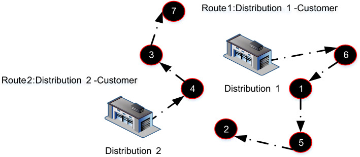
The numbers in this section are in the descending order to reach a permutation of these numbers (Figs. 3, 4, 5).

6	1	5	2	4	3	7	8	9	11	10
Route							Separators

Fig. 3.

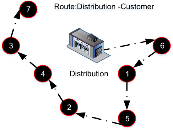
Distribution-customer route

Fig. 4.

Distribution-customer route

Fig. 5.

Vehicle allocation to factory

In this permutation, numbers greater than $\mathrm{Vc}$ are considered as separators, so that any series of numbers less than $\mathrm{Vc}$, which are placed in sequence, corresponding with a route starting from a facility and ending at the last point of that group. In this example, the created route starts from the first facility and ends with passing the route of $\left\{6,-,1,-,5,-,2,-,4,-,3,-,7\right\}$, represented as follows:

6	1	5	2	8	4	3	7	9	11	10
Route 1				Separator	Route 2			Separators

The solution includes two routes, the first one starting with the first facility and ending with {6-1-5-2}. The second one starts with the second facility and ends with {4-3-7}.

The second part of the N-length solution is associated with allocating the vehicles to the factories.

Vehicle
0.56	0.2	0.43
Vehicle section

The decimal numbers in this section are assigned to one of the factories:

$$⌊x,,\ast ,V,f,+,1⌋$$

$\mathit{Vf}$ denotes the number of factories.

2

2

2

The third part of the solution with the length of $Vd+N-1$ is corresponding with routing from factories to depots.

Factory → distribution
0.32	0.19	0.73	0.25	0.3	0.35	0.62
Routing from factory to (depot)

In this section, after sorting in descending order, the routes between the factories and depots are detected using the separators.

6	1	5	2	4	3	7
Separator	Route					Separator

In this example, a route can start from the second factory and pass {1-5-2-4-3}. In this section, it should be noted that any unused facilities, which were determined as useless facilities in the first section of the solution representation, will be removed from this route. Since only the first facility is used, the route links the second factory to the first facility and vice versa. After specifying the routes and factories, the amount of goods loaded at the beginning of the route, the amount of goods unloaded at each point and the distance between nodes (that has been passed by vehicles) can be distinguished. Finally, the fitness of each solution is determined.

Solution methods

The augmented epsilon constraint (AEC) method is employed to solve the proposed multiple objectives model using the GAMS software. In addition, two well-known metaheuristic MOGWO and NSGA-II algorithms are exploited to deal with the large-sized optimization problems.

The augmented epsilon constraint (AEC) METHOD

Numerous solutions, which are either poorly efficient or inconsistently efficient, are obtained through different $e_i$ values using the epsilon constraint (EC) method. The efficient solutions can be obtained through improving EC (Mavrotas, 2009). Initially, the proper intervals are found for every $e_i$ (Aghaei et al., 2011). The first objective function $(f_1)$ is the primary objective function. However, the second objective $(f_2)$ is confined to various amounts of ɛ, represented as follows:

$$\left\{\begin{array}{c}\mathrm{Min}z=f_1-{\varphi }_2.S_2\hfill \\ s.t.\hfill \\ x\in X\hfill \\ f_2\left(x\right)+s_2=e_2\hfill \end{array}\right)$$ 33

The NSGA-II algorithm

NSGA-II as a population-based algorithm inspired by the natures of genes has been utilized in numerous applications by many scholars because of its high performance and efficiency in solving optimization problems with multiple objectives. The function of this algorithm is based on the sorting of non-dominated solutions together with crossover and mutation operators defined as follows:

Crossover operator

Two parents are initially selected for reproduction. The parents are X₁ and X₂, respectively. Each parent is a string with a length of N. Then, a string with a length of N is randomly generated with numbers between zero and one called α.

Two children Y₁ and Y₂ are generated from these two parents, which have a share of each parent’s characteristics according to α. So, each gene of each child is created from as follows equation using parental genes.

$$Y_1=\alpha \times X_1+(1-\alpha )\times X_2$$ 34

$$Y_2=\alpha \times X_2+(1-\alpha )\times X_1$$ 35

Therefore, two children are generated inheriting from two parents.

Mutation operator

The mutation operator applies to the percentage of society members according to the mutation rate, and a new member is created in the mutated population. These members may be better or worse than society members. The mutation gives a chance to the algorithm to escape from convergence to local optimality. In this operator, after selecting a member for the mutation, a number of the genes are selected and randomly changed according to the mutation steps.

The MOGWO algorithm

MOGWO was introduced by Mirjalili et al. (2014); subsequently, it was modified to tackle multiple objectives optimization problems (Mirjalili et al., 2016). MOGWO pursues gray wolves’ hierarchical leadership and hunting operations in nature. A tribe of gray wolves are grouped into four categories named alpha (α), beta (β), delta (δ) and omega (ω) to organize hierarchical leadership and assign duties.

The first category is known as alpha (α) corresponding with the leader wolves who make decisions for the whole community. The following group is known as beta (β) corresponding with the wolves advising and assisting the α wolves with decision-making. The β wolves command the subordinate wolves. The third category is known as delta (δ) wolves that follow the α and β wolves. The δ wolves do scouting, guarding and hunting as their tasks and duties. The lowest group is known as omega (ω) wolves that follow the upper groups.

The mathematical programming model

The best candidate solutions of the single-objective model are known as alpha (α), likewise, the following suitable solution sets are known as beta (β), delta (δ), and omega (ω). However, for multiple objectives model, we need to define an archive set which keeps the non-dominated solutions until the final iteration.

Searching, siege and hunting prey

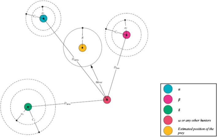
It is assumed that α, β, and δ groups bear more appropriate information about the possibilities of the prey positions. Therefore, the possible location is determined using the following equations considering the location of the α, β, and δ groups, and correspondingly the ω wolves update their positions, shown in Figs. 6 and 7. It should be noted that the random endpoint in a circle is determined by the α, β, and δ groups. In other words, the α, β, and δ groups approximate the prey’s location, and the other wolves update their positions correspondingly (Figs. 8, 9, 10, 11).

$$\overrightarrow{D_{\alpha }}=\left|\overrightarrow{C_1}\right)·\overrightarrow{X_{\alpha }}-\left(\overrightarrow{X}\right|$$

$$\overrightarrow{D_{\beta }}=\left|\overrightarrow{C_2}\right)·\overrightarrow{X_{\beta }}-\left(\overrightarrow{X}\right|$$

$$\overrightarrow{D_{\delta }}=\left|\overrightarrow{C_2}\right)·\overrightarrow{X_{\delta }}-\left(\overrightarrow{X}\right|$$

$$\overrightarrow{X_1}=\overrightarrow{X_{\alpha }}-\overrightarrow{A_1}·(\overrightarrow{D_{\alpha }})$$

$$\overrightarrow{X_2}=\overrightarrow{X_{\beta }}-\overrightarrow{A_2}·\left(\overrightarrow{D_{\beta }}\right)$$

$$\overrightarrow{X_3}=\overrightarrow{X_{\delta }}-\overrightarrow{A_3}·(\overrightarrow{D_{\delta }})$$

$$\overrightarrow{X}\left(t,+,1\right)=\frac{\overrightarrow{X_1}+\overrightarrow{X_2}+\overrightarrow{X_3}}{3}$$ 36

Fig. 6.

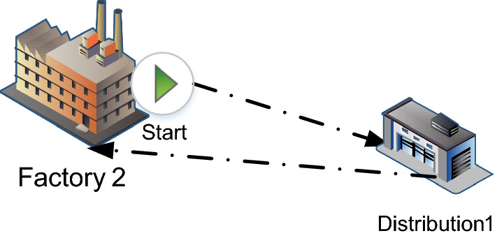
Factory-distribution route

Fig. 7.

Fitness-based crossover example

Fig. 8.

Swap mutation

Fig. 9.

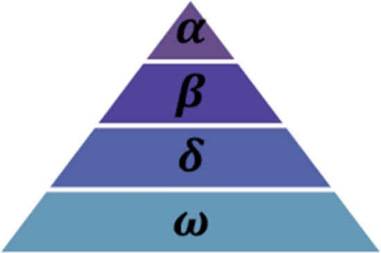
The hierarchy of the gray wolf society

Fig. 10.

Hunting location and updating the location of the ω wolves

Fig. 11.

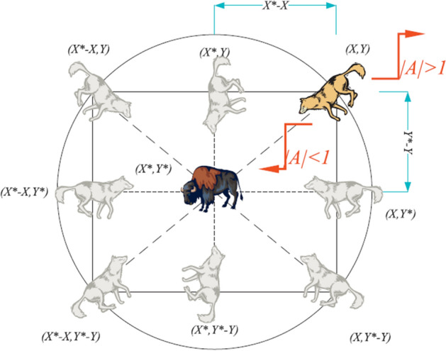
Changing wolf location regarding various α values

The A and C values are acquired using the below equations:

$$\overrightarrow{A}=2\overrightarrow{a}·\overrightarrow{r_1}-\overrightarrow{a},$$

$$\overrightarrow{C}=2·\overrightarrow{r_2},$$ 37

where a is linearly reduced from 2 to 0 throughout the algorithm iterations. r₁ and r₂ are also random vectors between 0 and 1. The prey location relies on the X₁, X₂, and X₃ values that depend on the α, β, and δ positions. Exploration is ascertained by A values that are greater than 1 or lower than − 1. Exploration is also ensured by C values that are between 0 and 2. Any C value greater than 1 indicates that the hunting location is accentuated to specify the required distance for the movement of the search agent. Any C value less than 1 indicates that the hunting location is paid less attention. Unlike A, the domain of C is not decreased so that search carries on until the last iteration. Therefore, A and C guarantee that the algorithm is not trapped in the local optimal solutions (Mirjalili et al., 2016).

Results and discussion

Model validation

The proposed bi-objective mathematical programming model is implemented on a set of standard problems to compare its final solutions with the previous studies. These standard location-routing problems are known as the Sterle1 problem set. The details of the 26-node (I2-15 × 8 × 3) Gaskell problem are presented as follows (with a slight change from the main parameters). In this problem, there are three factories with the same capacity of 7530 in the first echelon, shown with indices 1 to 3. In the second echelon, there are eight potential locations for depots, shown in indices 4 to 11. The capacities of the depots are 6000, 5600, 5700, 5600, 4700, 5400, 5000 and 4300 units, respectively, and the costs of establishing each depot are 75, 75, 75, 75, 65, 70, 55 and 55 units, respectively. The problem involves 15 customers with known amounts of demands. The spatial coordinates of all 26 network nodes are specified, and the Euclidean distances between nodes are determined. The echelon-one transport fleet is heterogeneous and limited in number, and three different types of vehicles (one for each type) are available for each factory (the parameters are given in Table 3). The echelon-two transport fleet is identical with an unlimited number for each depot (the parameters are given in Table 4).

Table 3.

Parameters related to the echelon-one vehicles

Vehicle index (n)		n1	n2	n3
${{\mathit{Co}}_{2}ef}_n$	(kg CO2/km)	0.51976	0.68395	1.09749
${{\mathit{Co}}_{2}f1}_n$	(kg CO2/km)	0.44276	0.53196	0.76266
Capacity	${CN1}_n$	4000	8000	17,000
Fixed cost	${FC1}_n$	10	20	30

Table 4.

Parameters related to the echelon-two vehicles

Vehicle index (n)		n1	n2	n3
${{\mathit{Co}}_{2}es}_n$	(kg CO2/km)	0.44276	0.44276	0.44276
${{\mathit{Co}}_{2}fs2}_n$	(kg CO2/km)	0.51976	0.51976	0.51976
Capacity	${CN2}_n$	2000	2000	2000
Fixed cost	${FC2}_n$	40	40	40

The model was coded in GAMS optimization software version 24.1.2 and solved by using the CPLEX optimizer on a laptop with Corei7 processor, 6 GB RAM, and 64-bit operating system. First, the problem was solved considering the single objective function of minimizing the total cost to find the optimal value of the first objective function (Z₁^* = 595). Then, the problem was solved taking the second objective function of minimizing the amount of CO₂ emissions into consideration to obtain the optima value of the second objective function (Z₂^* = 137.297).

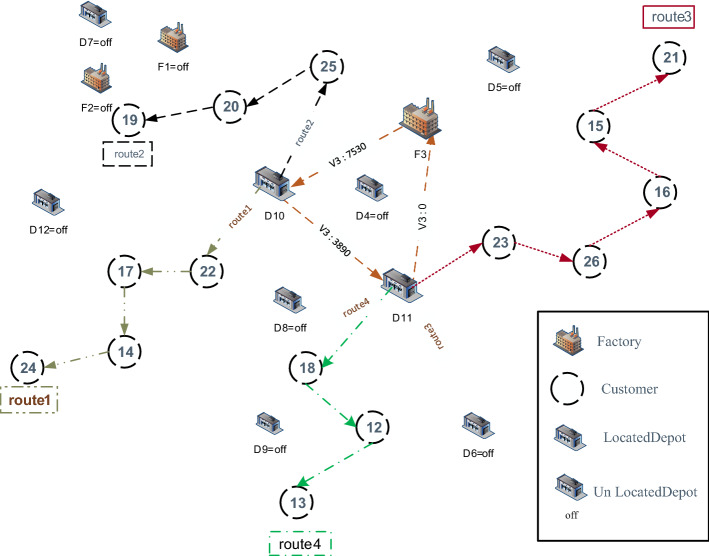
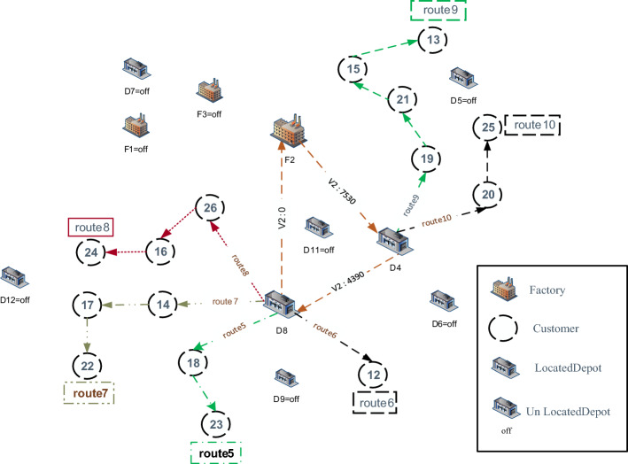
Figures 12 and 13 depict the results obtained by solving the model in the form of the graphical representations of the routes in both levels corresponding with the optimal value of each objective function. Figure 14 shows the Pareto frontier considering the trade-off between objective functions.

Fig. 12.

Graph of the optimal value of the first objective function

Fig. 13.

Graph of the optimal value of the second objective function

Fig. 14.

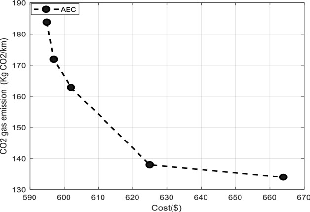
Pareto frontier corresponding with the trade-off between the objective functions of the problem

Comparison of AEC and two metaheuristic algorithms

A set of standard examples has been used to solve and test the proposed model as well as the comparability of the final model with other previous research. These standard problems relate to the location-routing problem known as the Gaskell problem set. Full details of this set of problem are available on OR-Library website. The details of Gaskell's problem with 29 customers are described in full as follows.

At the first echelon, there are two factories with capacities of 8000 and 11,000 which are represented by node indices of 1 to 2. At the second echelon, there are also five potential locations for depot establishment shown by node indexes of 3 to 7. The capacity of all depots is 5000 units, and the cost of establishing each depot is 150 monetary units. The problem consists of 29 customers with known demand values, along with the location specifications of all 36 specified network nodes and intervals are calculated based on Euclidean distance matrix. The transport fleet in the first echelon is heterogeneous and limited in number, and each factory has three different types of vehicles (of each type). Details of these vehicles are shown in Table 5. The second echelon fleet is the same with an unlimited number of depots. Details of these vehicles are presented in Table 6.

Table 5.

Parameters related to the first echelon vehicles

Vehicle index (n)		n1	n2	n3
${{\mathit{Co}}_{2}ef}_n$	(kg CO2/km)	0.51219	0.63789	0.75783
${{\mathit{Co}}_{2}f1}_n$	(kg CO2/km)	0.60127	0.82015	1.09053
Capacity	${CN1}_n$	5000	10,000	20,000
Fixed cost	${FC1}_n$	40	50	60

Table 6.

Parameters related to the second echelon vehicles

Vehicle index (n)		n1	n2	n3
${{\mathit{Co}}_{2}es}_n$	(kg CO2/km)	0.51976	0.51976	0.51976
${{\mathit{Co}}_{2}fs2}_n$	(kg CO2/km)	0.60127	0.60127	0.60127
Capacity	${CN2}_n$	4500	4500	4500
Fixed cost	${FC2}_n$	100	100	100

The problem was solved by using AEC exact method, and the results were compared to the results obtained by the MOGWO and NSGAII metaheuristic algorithms (shown in Table 7 and 8). As Fig. 15 displays, the metaheuristic algorithms achieved close to the optimal solutions using the appropriate solution representation (expressed in Sect. 4.2).

Table 7.

The obtained values of two objective functions through three applied solution methods

NSGA-II		AEC		MOGWO
679	115.8483	782	105.02	468	168.7304
699	112.1978	762	108.058	799	109.5695
512	116.6538	752	110.857	479	127.905
491	124.4934	699	112.811
480	128.8366	509	118.121
		489	122.93
		479	127.363
		475	157.536
		465	167.802

Table 8.

The outputs of MOGWO and NSGA-II algorithms

Problem	MOGWO					NSGA-II
	Diversity	Spacing	MID	SNS	RAS	Diversity	Spacing	MID	SNS	RAS
1	1067.512	148.0999	1273.004	277.531	0.00811	990.4074	199.6093	1404.025	346.799	0.03867
2	316.2981	2.48088	1265.273	78.1097	0.00359	381.5408	46.71573	1532.677	112.139	0.0221
3	284.7204	28.51128	2062.551	97.3117	0.01647	566.0067	85.011	1975.405	142.101	0.03474
4	742.8233	172.1164	2546.159	253.404	0.01017	369.1774	57.72906	3081.734	87.8945	0.05306
5	1440.891	183.4763	3624.138	420.524	0.02732	364.6286	6.15797	5343.917	87.0728	0.03117
6	905.5452	155.0269	4835.443	238.217	0.00521	566.9397	20.8887	4896.61	88.419	0.03727
7	1673.548	218.5225	6038.501	523.458	0.00864	1296.01	132.767	6625.508	300.78	0.0444
8	1587.31	272.7807	7242.698	456.747	0.00391	1115.096	80.56163	6991.314	170.291	0.02992
9	1893.705	331.7994	8283.348	465.134	0.0106	761.2552	89.94587	8816.237	141.41	0.03325
10	2948.851	360.8961	9790.272	760.343	0.01362	1238.795	105.2938	10,247.29	248.41	0.03557
11	3213.331	612.2821	11,062.07	882.292	0.00601	857.6919	53.95048	11,292.32	179.192	0.06296
12	2622.548	187.4369	11,663.58	445.646	0.00036	595.5531	31.36583	11,605.89	21.1353	0.02176
13	2472.523	458.6644	12,767.46	484.493	0.0082	1041.193	100.9963	13,580.33	57.0764	0.03838
14	4026.231	442.0236	14,221.69	707.905	0.00924	1011.746	122.8333	14,460.76	214.857	0.02631
15	3990.497	663.0106	15,744.93	940.091	0.01508	1218.572	111.6671	17,261.99	336.124	0.02407
16	4650.012	600.1525	16,652.86	1055.76	0.0104	1216.606	83.32716	17,017.1	162.991	0.03064
17	5531.21	688.19	17,859.23	10,958	0.01091	1355.731	92.732	18,968.12	198.23	0.30589
18	7266.041	605.8527	19,705.05	1541.75	0.00538	1818.935	274.5804	22,518.76	395.62	0.02438
19	7313.862	451.1099	21,481.39	1348.67	0.0026	1648.871	221.8919	21,865.5	217.335	0.0219
20	5689.245	459.6758	21,372.85	1053.96	0.01358	1373.061	260.498	22,882.63	413.077	0.02085
21	9956.733	766.6807	28,595.09	1424.55	0.00578	1114.823	114.0908	29,711.8	179.44	0.01863
22	10,938.39	851.1795	34,413.57	1282.59	0.00875	1795.892	479.8888	36,398.59	292.267	0.01599
Average	3660.538	393.635	12,386.42	1168.02	0.00927	1031.751	126.0228	13,112.66	199.666	0.04418

Fig. 15.

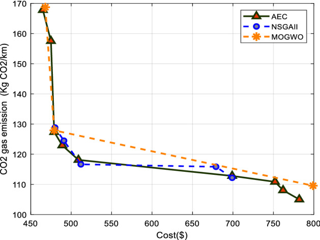
Pareto frontier of three solution methods

Sensitivity analysis

Sensitivity analysis means finding the trend and amount of changes in the values of the objective functions with respect to the changes in the given parameters of the problem. It is logical that these analyzes are limited only to the parameters under the control of the decision maker. In this section, Figs. 16, 17, 18, 19 show the results of the sensitivity analysis conducted on the amount of parameters such as the capacity of depots and the number of secondary vehicles.

Fig. 16.

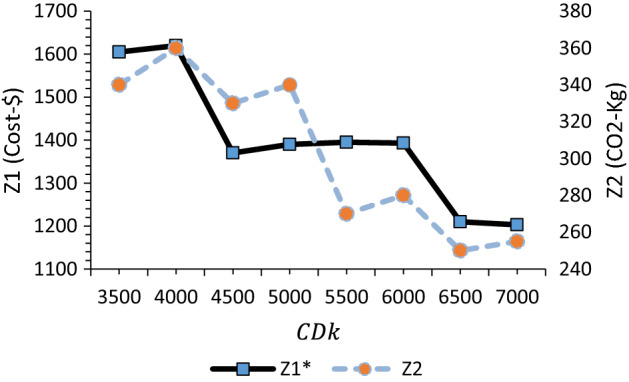
The effect of changing depot capacity on the optimal amount of cost and corresponding CO₂ emission

Fig. 17.

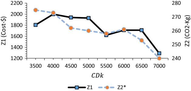
The effect of changing depot capacity on the optimal amount of CO₂ emission and corresponding amount of cost

Fig. 18.

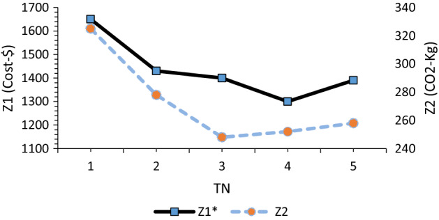
The effect of changing the number of secondary vehicles on the optimal amount of cost and corresponding CO₂ emission

Fig. 19.

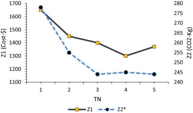
The effect of changing the number of secondary vehicles on the optimal amount of CO₂ emission and corresponding amount of cost

The analysis demonstrates that the more the capacity of the intermediate facilities increases, the less the amount of cost and pollution, because the need to build new distribution centers for providing customer service decreases and the smaller number of distribution centers would be built. On the other hand, when the capacity of distribution centers is low, vehicles have to travel more distances, and sometimes the optimal loading capacity cannot be used.

Also, if the number of available vehicles (TN) increases, in other words, the company is able to acquire more vehicles, this will be effective in reducing cost and pollution, as optimal loading can be done with a reasonable tradeoff between cost and pollution.

Evaluation indices

In this section, the outputs of the two MOGWO and NSGA-II algorithms presented in Table 5 are evaluated and compared. For a single objective (minimizing $Z_1$) problem, any solution with lower $Z_1$ value is more desirable. However, the following indices were defined to evaluate and compare the performance of solution methods for multiple objectives optimization problems (Jolai et al., 2013).

Diversification matrix (DM) index

This index is obtained using the below formula. Greater values are more desirable (Jolai et al., 2013).

$$DM=\sqrt{{({\max f}_{1i}-\min f_{1i})}^2+{({\max f}_{2i}-\min f_{2i})}^2}$$ 38

Mean ideal distance (MID) index

A desirable solution for the problem is initially presumed; subsequently, the mean of deviations of the Pareto solutions from the desirable solution is computed (Behnamian et al., 2009). This index is acquired using the following equation (Jolai et al., 2013):

$$\mathrm{MID}=\frac{{\sum }_{i=1}^n{c}_i}{n}$$ 39

where n indicates the number of solutions of the Pareto set and the $c_i$ value is calculated using the following formula (Jolai et al., 2013):

$$c_i=\sqrt{f_{1i}^2+f_{2i}^2}$$ 40

Spacing (S)

The S performance metric, which is calculated through following equation, gives an indication of the evenness of solutions obtained from an algorithm (Kaveh & Mahdavi, 2019). A lower value of S shows a more uniform distribution of the obtained non-dominated solutions.

$$S={\left(\frac{1}{n_{\mathit{pf}}},{\sum }_{i=1}^{n_{\mathit{pf}}},{(d_i-\overline{d})}^2\right)}^{\frac{1}{2}},\text{where}\overline{d}=\frac{1}{n_{\mathit{pf}}}{\sum }_{i=1}^{n_{\mathit{pf}}}{d}_i$$ 41

Spread of non-dominance solutions (SNS)

The greater SNS value as the diversity index the superior the algorithm is. This index is determined using the below equation (Jolai et al., 2013):

$$\text{SNS}=\sqrt{\frac{{\sum }_{i=1}^n{(\text{MID}-c_i)}^2}{n-1}}$$ 42

The rate of achievement to two objectives simultaneously (RAS)

The RAS index is defined by the following equation (Mirjalili et al., 2016):

$$\text{RAS}=\frac{{\sum }_{i=1}^n\left(\frac{f_{1i}-F_i}{F_i}\right)+\left(\frac{f_{2i}-F_i}{F_i}\right)}{n}.$$ 43

Analysis and discussion

After the evaluation indexes were defined in the previous section, 22 test problems were designed to measure the algorithms’ performance. Then, each problem is run 10 times for each algorithm and the average is reported as the final answer for the given algorithm. The values of all parameters for the MOGWO and NSGA-II algorithm are shown in Table 7.

The outputs of two algorithms are subsequently analyzed regarding Table 8.

The diversity index

The performance of two algorithms in terms of this index is displayed in Fig. 20 demonstrating that MOGWO performs better than NSGA-II.

Fig. 20.

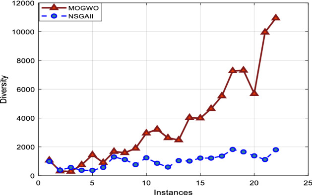
Comparison of two algorithms in terms of diversity index

The MID index

For the MID index (the less value the better performance) as shown in Fig. 21, some results of the MOGWO algorithm are better than the ones of NSGA-II.

Fig. 21.

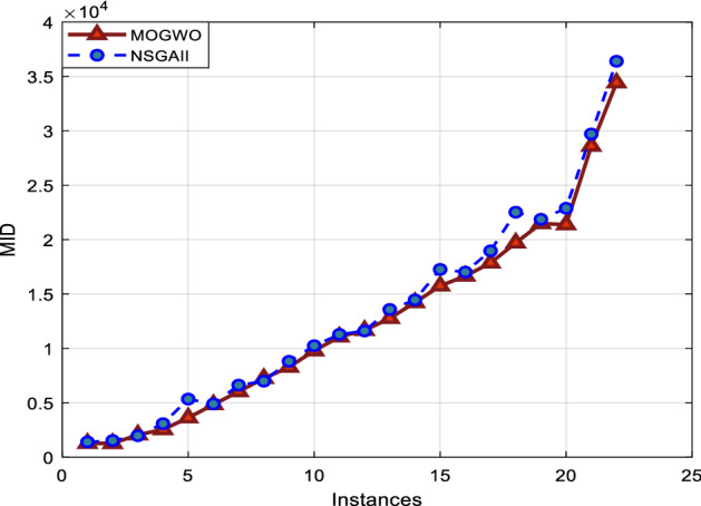
Comparison of two algorithms in terms of MID index

The Spacing index

As shown in Fig. 22, the NSGA-II algorithm performs better than the MOGWO algorithm.

Fig. 22.

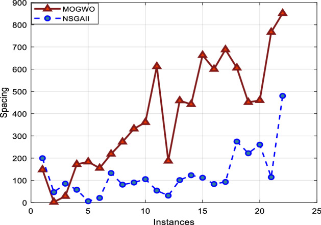
Comparison of two algorithms in terms of spacing index

The SNS index

The higher the SNS index, the better performance. As seen in Fig. 23, the MOGWO algorithm outperforms the NSGA-II algorithm.

Fig. 23.

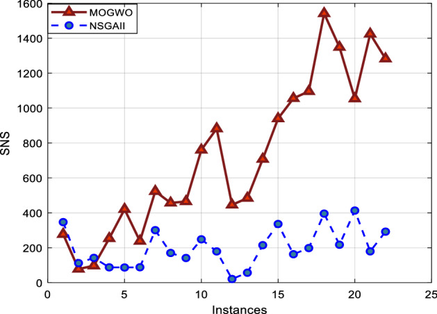
Comparison of two algorithms in terms of SNS index

The RAS index

The less the RAS index, the better performance. As shown in Fig. 24, the MOGWO algorithm performs better.

Fig. 24.

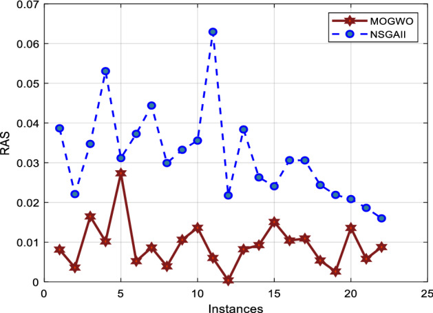
Comparison of two algorithms in terms of RAS index

According to the evaluation, Figs. 20, 21, 22, 23, 24 and the characteristics of the indicators, it can be concluded that the MOGWO algorithm is superior in terms of three indexes and there is no meaningful difference in terms of MID index. Also, in terms of one index, NSGAII has a better performance; therefore, it can be stated that the MOGWO algorithm has a better performance than the NSGAII algorithm.

Conclusions

In this paper, a bi-objective mixed integer linear programming (MILP) model was presented for hybrid two-echelon closed and open locating-routing problems (2E-COLRP) with the objectives of minimizing total cost and CO₂ emission of the entire transportation. The contribution of this mathematical model is in combining closed and open routes in a two-echelon location-routing problem, such that the first echelon routes are closed type (each journey must end at its starting point, which is a factory) and second echelon routes are open routes (after satisfying the last customer's demand, vehicle does not return to the first depot). In addition, in order to consider the real world conditions, the problem was modeled and solved with two objectives of minimizing the total cost and CO₂ emission.

Due to the conflicting objectives of the problem, the problem was solved using EC method to obtain the Pareto front diagram. This graph shows the varying amount of both objective functions from the optimality of each one to the optimality of the other one. Decision-makers determine which goal has more priority, so that the appropriate value of one goal can be achieved by slightly ignoring the optimal value of the other goal. Hence, this facilitates the decision-making process in different situations.

According to the average of all outputs, the MOGWO algorithm outperformed in terms of four MID, diversity, RAS, and SNS indices. However, the NSGA-II algorithm performed better in terms of the spacing index only.

The obtained results of sensitivity analysis related to the depot capacity and number of secondary vehicles generally indicate that by increasing the depot capacity and number of secondary vehicles, the values of both objective functions are reduced and the optimal state is obtained. The model was presented in this study without any time dependence and constraints such as time windows. Time windows for customers can be considered as a suggestion for future research.

Appendix 1: Symbol definition

Definition	Abbreviation
2E-COLRP	Two-echelon close and open location-routing problem
AEC	Augmented epsilon constraint method
VRP	The vehicle routing problem
2E-LRP	Two-echelon location-routing problem
OVRP	Open vehicle routing problem
COMVRP	Closed–open-mixed-vehicle-routing-problem
DM	Diversification matrix
MID	Mean ideal distance
S	Spacing
SNS	Spread of non-dominance solutions
RAS	The rate of achievement to two objectives simultaneously
NSGAII	Non-dominated sorting genetic algorithm
MOGWO	Multi-objective grey wolf optimizer

References

- Abbassi A, Kharraja S, El Hilali Alaoui A, Boukachour J, Paras D. Multi-objective two-echelon location-distribution of non-medical products. International Journal of Production Research. 2021;59(17):5284–5300. doi: 10.1080/00207543.2020.1777479. [DOI] [Google Scholar]
- Aghaei J, Amjady N, Shayanfar HA. Multi-objective electricity market clearing considering dynamic security by lexicographic optimization and augmented epsilon constraint method. Applied Soft Computing Journal. 2011;11(4):3846–3858. doi: 10.1016/j.asoc.2011.02.022. [DOI] [Google Scholar]
- Amiri M, Amin SH, Tavakkoli-Moghaddam R. A Lagrangean decomposition approach for a novel two-echelon node-based location-routing problem in an offshore oil and gas supply chain. Transportation Research Part E: Logistics and Transportation Review. 2019;128:96–114. doi: 10.1016/j.tre.2019.05.014. [DOI] [Google Scholar]
- Atefi R, Salari M, Coelho CL, Renaud J. The open vehicle routing problem with decoupling points. European Journal of Operational Research. 2018;265(1):316–327. doi: 10.1016/j.ejor.2017.07.033. [DOI] [Google Scholar]
- Babaee, E., Abbasian, P., & Weber, G. (2020). Since January 2020 Elsevier has created a COVID-19 resource centre with free information in English and Mandarin on the novel coronavirus COVID-19.
- Bauer J, Bektaş T, Crainic TG. Minimizing greenhouse gas emissions in intermodal freight transport: An application to rail service design. Journal of the Operational Research Society. 2010;61(3):530–542. doi: 10.1057/jors.2009.102. [DOI] [Google Scholar]
- Behnamian J, Ghomi SF, Zandieh M. A multi-phase covering Pareto-optimal front method to multi-objective scheduling in a realistic hybrid flowshop using a hybrid metaheuristic. Expert Systems with Applications. 2009;36(8):11057–11069. doi: 10.1016/j.eswa.2009.02.080. [DOI] [Google Scholar]
- Bektaş T, Laporte G. The pollution-routing problem. Transportation Research Part B: Methodological. 2011;45(8):1232–1250. doi: 10.1016/j.trb.2011.02.004. [DOI] [Google Scholar]
- Biuki M, Kazemi A, Alinezhad A. An integrated location-routing-inventory model for sustainable design of a perishable products supply chain network. Journal of Cleaner Production. 2020 doi: 10.1016/j.jclepro.2020.120842. [DOI] [Google Scholar]
- Cao E, Lai M, Yang H. Open vehicle routing problem with demand uncertainty and its robust strategies. Expert Systems with Applications. 2014;41(7):3569–3575. doi: 10.1016/j.eswa.2013.11.004. [DOI] [Google Scholar]
- Cao JX, Wang X, Gao J. A two-echelon location-routing problem for biomass logistics systems. Biosystems Engineering. 2021;202:106–118. doi: 10.1016/j.biosystemseng.2020.12.007. [DOI] [Google Scholar]
- Crainic, T. G., Mancini, S., Perboli, G., & Tadei, R. (2011). "Multi-start heuristics for the two-echelon vehicle routing problem. In European conference on evolutionary computation in combinatorial optimization (pp. 179–190). Springer.
- Dai Z, Aqlan F, Gao K, Zhou Y. A two-phase method for multi-echelon location-routing problems in supply chains. Expert Systems with Applications. 2019;115:618–634. doi: 10.1016/j.eswa.2018.06.050. [DOI] [Google Scholar]
- Darvish M, Archetti C, Coelho LC, Speranza MG. Flexible two-echelon location routing problem. European Journal of Operational Research. 2019;277(3):1124–1136. doi: 10.1016/j.ejor.2019.04.002. [DOI] [Google Scholar]
- Dawei Z, Hamid ABA, Chin TA, Leng KC. Green supply chain management: A literature review. Sains Humanika. 2015;5(2):20. doi: 10.11113/sh.v5n2.624. [DOI] [Google Scholar]
- Dewi SK, Utama DM. A new hybrid whale optimization algorithm for green vehicle routing problem. Systems Science and Control Engineering. 2021;9(1):61–72. doi: 10.1080/21642583.2020.1863276. [DOI] [Google Scholar]
- Diabat A, Al-Salem M. An integrated supply chain problem with environmental considerations. International Journal of Production Economics. 2015;164(330–338):2015. [Google Scholar]
- Ebrahimi SB. A stochastic multi-objective location-allocation-routing problem for tire supply chain considering sustainability aspects and quantity discounts. Journal of Cleaner Production. 2018;198:704–720. doi: 10.1016/j.jclepro.2018.07.059. [DOI] [Google Scholar]
- Fagerholt, K., Laporte, G., & Norstad, I. (2010). Reducing fuel emissions by optimizing speed on shipping routes. Journal of the Operational Research Society,61(3), 523–529.
- Fallahtafti A, Ardjmand E, Young WA, Weckman GR. A multi-objective two-echelon location-routing problem for cash logistics: A metaheuristic approach. Applied Soft Computing. 2021;111:107685. doi: 10.1016/j.asoc.2021.107685. [DOI] [Google Scholar]
- Fleszar K, Osman IH, Hindi KS. A variable neighbourhood search algorithm for the open vehicle routing problem. European Journal of Operational Research. 2009;195(3):803–809. doi: 10.1016/j.ejor.2007.06.064. [DOI] [Google Scholar]
- Gao, J. C. X. W. B. L. and J., and 1Institute. (2020). Cictp 2020 1366. The location-routing problem: A review Jinxin, 1366–1377.
- Guo H, Li C, Zhang Y, Zhang C, Wang Y. A nonlinear integer programming model for integrated location, inventory, and routing decisions in a closed-loop supply chain. Complexity. 2018;2018:2726070. doi: 10.1155/2018/2726070. [DOI] [Google Scholar]
- Jacobsen SK, Madsen OB. A comparative study of heuristics for a two-echelon routing-location problem. European Journal of Operational Research. 1980;5(6):378–387. doi: 10.1016/0377-2217(80)90124-1. [DOI] [Google Scholar]
- Jolai F, Asefi H, Rabiee M, Ramezani P. Bi-objective simulated annealing approaches for no-wait two-stage flexible flow shop scheduling problem. Scientia Iranica. 2013;20(3):861–872. [Google Scholar]
- Kaveh A, Mahdavi VR. Multi-objective colliding bodies optimization algorithm for design of trusses. Journal of Computational Design and Engineering. 2019;6(1):49–59. doi: 10.1016/j.jcde.2018.04.001. [DOI] [Google Scholar]
- Khan SH, Chouhan VK, Srinivasan S. A multi-objective optimization of closed-loop supply chain problem with vehicle routing. Global Journal of Engineering and Technology Advances. 2021;6(2):121–130. doi: 10.30574/gjeta.2021.6.2.0009. [DOI] [Google Scholar]
- Kumar RS, Kondapaneni K, Dixit V, Goswami A, Thakur LS, Tiwari MK. Multi-objective modeling of production and pollution routing problem with time window: A self-learning particle swarm optimization approach. Computers & Industrial Engineering. 2016;99:29–40. doi: 10.1016/j.cie.2015.07.003. [DOI] [Google Scholar]
- Lalla-Ruiz E, Mes M. Mathematical formulations and improvements for the multi-depot open vehicle routing problem. Optimization Letters. 2021;15(1):271–286. doi: 10.1007/s11590-020-01594-z. [DOI] [Google Scholar]
- Lin JR, Lei HC. Distribution systems design with two-echelon routing considerations. Annals of Operations Research. 2009;172(1):329. doi: 10.1007/s10479-009-0628-y. [DOI] [Google Scholar]
- Liu A, Zhu Q, Xu L, Lu Q, Fan Y. Sustainable supply chain management for perishable products in emerging markets: An integrated location-inventory-routing model. Transportation Research Part E: Logistics and Transportation Review. 2021;150:1–19. doi: 10.1016/j.tre.2021.102319. [DOI] [Google Scholar]
- Liu R, Jiang Z. The close–open mixed vehicle routing problem. European Journal of Operational Research. 2012;220(2):349–360. doi: 10.1016/j.ejor.2012.01.061. [DOI] [Google Scholar]
- Lu Y, Lang M, Yu X, Li S. A sustainable multimodal transport system: The two-echelon location-routing problem with consolidation in the Euro-China expressway. Sustainability (Switzerland) 2019;11(19):1–25. doi: 10.3390/su11195486. [DOI] [Google Scholar]
- Maden W, Eglese R, Black D. Vehicle routing and scheduling with time-varying data: A case study. Journal of the Operational Research Society. 2010;61(3):515–522. doi: 10.1057/jors.2009.116. [DOI] [Google Scholar]
- Martínez-Salazar IA, Molina J, Ángel-Bello F, Gómez T, Caballero R. Solving a bi-objective transportation location routing problem by metaheuristic algorithms. European Journal of Operational Research. 2014;234(1):25–36. doi: 10.1016/j.ejor.2013.09.008. [DOI] [Google Scholar]
- Masoudipour E, Jafari A, Amirian H, Sahraeian R. A novel transportation location routing network for the sustainable closed-loop supply chain considering the quality of returns. Journal of Remanufacturing. 2020;10(2):79–106. doi: 10.1007/s13243-019-00075-6. [DOI] [Google Scholar]
- Mavrotas G. Effective implementation of the e-constraint method in Multi-Objective Mathematical Programming problems. Applied Mathematics and Computation. 2009;213(2):455–465. doi: 10.1016/j.amc.2009.03.037. [DOI] [Google Scholar]
- McKinnon, A. (2007). “CO2 emissions from freight transport: an analysis of UK data”. In Logistics Research Network-2007 Conference Global Supply Chains: Developing Skills, Capabilities and Networks.
- Melo MT, Nickel S, Saldanha-Da-Gama F. Facility location and supply chain management: A review. European Journal of Operational Research. 2009;196(2):401–412. doi: 10.1016/j.ejor.2008.05.007. [DOI] [Google Scholar]
- MirHassani SA, Abolghasemi N. A particle swarm optimization algorithm for open vehicle routing problem. Expert Systems with Applications. 2011;38(9):11547–11551. doi: 10.1016/j.eswa.2011.03.032. [DOI] [Google Scholar]
- Mirjalili, S., Mirjalili, S. M., Lewis, A., & Optimizer, G. W. (2014). Advances in engineering software. Renewable and Sustainable Energy Reviews, 46–61.
- Mirjalili S, Saremi S, Mirjalili SM, Coelho LDS. Multi-objective grey wolf optimizer: A novel algorithm for multi-criterion optimization. Expert Systems with Applications. 2016;47:106–119. doi: 10.1016/j.eswa.2015.10.039. [DOI] [Google Scholar]
- Mohammed MA, Ghani MKA, Hamed RI, Mostafa SA, Ahmad MS, Ibrahim DA. Solving vehicle routing problem by using improved genetic algorithm for optimal solution. Journal of Computational Science. 2017;21:255–262. doi: 10.1016/j.jocs.2017.04.003. [DOI] [Google Scholar]
- Navazi F, Sazvar Z, Tavakkoli-Moghaddam R. A sustainable closed-loop location-routing-inventory problem for perishable products. Scientia Iranica. 2021;10:20. doi: 10.24200/sci.2021.55642.4353. [DOI] [Google Scholar]
- Navazi F, Sedaghat A, Tavakkoli-Moghaddam R. A new sustainable location-routing problem with simultaneous pickup and delivery by two-compartment vehicles for a perishable product considering circular economy. IFAC-PapersOnLine. 2019;52(13):790–795. doi: 10.1016/j.ifacol.2019.11.212. [DOI] [Google Scholar]
- Nguyen VP, Prins C, Prodhon C. Solving the two-echelon location routing problem by a GRASP reinforced by a learning process and path relinking. European Journal of Operational Research. 2012;216(1):113–126. doi: 10.1016/j.ejor.2011.07.030. [DOI] [Google Scholar]
- Niu Y, Yang Z, Chen P, Xiao J. Optimizing the green open vehicle routing problem with time windows by minimizing comprehensive routing cost. Journal of Cleaner Production. 2018;171:962–971. doi: 10.1016/j.jclepro.2017.10.001. [DOI] [Google Scholar]
- Norouzi N, Tavakkoli-Moghaddam R, Ghazanfari M, Alinaghian M, Salamatbakhsh A. A new multi-objective competitive open vehicle routing problem solved by particle swarm optimization. Networks and Spatial Economics. 2012;12(4):609–633. doi: 10.1007/s11067-011-9169-4. [DOI] [Google Scholar]
- Ouhader H, Elkyal M. Combining facility location and routing decisions in sustainable urban freight distribution under horizontal collaboration: how can shippers be benefited? Mathematical Problems in Engineering. 2017 doi: 10.1155/2017/8687515. [DOI] [Google Scholar]
- Pichka K, Bajgiran AH, Petering ME, Jang J, Yue X. The two echelon open location routing problem: Mathematical model and hybrid heuristic. Computers & Industrial Engineering. 2018;121:97–112. doi: 10.1016/j.cie.2018.05.010. [DOI] [Google Scholar]
- Prodhon C, Prins C. A survey of recent research on location-routing problems. European Journal of Operational Research. 2014;238(1):1–17. doi: 10.1016/j.ejor.2014.01.005. [DOI] [Google Scholar]
- Pronello, C., & André, M. (2000). Pollutant emissions estimation in road transport models. INRETS-LTE report, 2007.
- Purnawan RA, Zagloel TYM, Ardi R. Closed-loop supply chain optimization with vehicle routing problem for gallon water distribution. ACM International Conference Proceeding Series. 2018 doi: 10.1145/3288155.3288163. [DOI] [Google Scholar]
- Rabbani M, Navazi F, Farrokhi-Asl H, Balali MH. A sustainable transportation-location-routing problem with soft time windows for distribution systems. Uncertain Supply Chain Management. 2018;6(3):229–254. doi: 10.5267/j.uscm.2017.12.002. [DOI] [Google Scholar]
- Rahmani A. A new closed–open vehicle routing approach in stochastic environments. International Journal of Computer Mathematics: Computer Systems Theory. 2021;6(2):113–129. doi: 10.1080/23799927.2020.1861660. [DOI] [Google Scholar]
- Rahmani Y, Ramdane Cherif-Khettaf W, Oulamara A. The two-echelon multi-products location-routing problem with pickup and delivery: Formulation and heuristic approaches. International Journal of Production Research. 2016;54(4):999–1019. doi: 10.1080/00207543.2015.1040127. [DOI] [Google Scholar]
- Rahmani Hosseinabadi, A. A., Zolfagharian, A., & Alinezhad, P. (2021). An efficient hybrid meta-heuristic algorithm for solving the open vehicle routing problem. In Studies in fuzziness and soft computing (Vol. 393, pp. 257–274). Springer. 10.1007/978-3-030-47124-8_21
- Repoussis PP, Tarantilis CD, Bräysy O, Ioannou G. A hybrid evolution strategy for the open vehicle routing problem. Computers & Operations Research. 2010;37(3):443–455. doi: 10.1016/j.cor.2008.11.003. [DOI] [Google Scholar]
- Ruiz E, Soto-Mendoza V, Ruiz Barbosa AE, Reyes R. Solving the open vehicle routing problem with capacity and distance constraints with a biased random key genetic algorithm. Computers and Industrial Engineering. 2019;133:207–219. doi: 10.1016/j.cie.2019.05.002. [DOI] [Google Scholar]
- Ruiz y Ruiz, E., García-Calvillo, I., and Nucamendi-Guillén, S. Open vehicle routing problem with split deliveries: Mathematical formulations and a cutting-plane method. Operational Research. 2020 doi: 10.1007/s12351-020-00580-8. [DOI] [Google Scholar]
- Salhi S, Rand GK. The effect of ignoring routes when locating depots. European Journal of Operational Research. 1989;39(2):150–156. doi: 10.1016/0377-2217(89)90188-4. [DOI] [Google Scholar]
- Sbihi A, Eglese RW. Combinatorial optimization and green logistics. 4OR. 2007;5(2):99–116. doi: 10.1007/s10288-007-0047-3. [DOI] [Google Scholar]
- Soleimani H, Govindan K, Saghafi H, Jafari H. Fuzzy multi-objective sustainable and green closed-loop supply chain network design. Computers & Industrial Engineering. 2017;109:191–203. doi: 10.1016/j.cie.2017.04.038. [DOI] [Google Scholar]
- Soto-Mendoza V, García-Calvillo I, Ruiz-y-Ruiz E, Pérez-Terrazas J. A hybrid grasshopper optimization algorithm applied to the open vehicle routing problem. Algorithms. 2020 doi: 10.3390/A13040096. [DOI] [Google Scholar]
- Srivastava SK. Green supply-chain management: A state-of-the-art literature review. International Journal of Management Reviews. 2007;9(1):53–80. doi: 10.1111/j.1468-2370.2007.00202.x. [DOI] [Google Scholar]
- Subramanian A, Uchoa E, Ochi LS. A hybrid algorithm for a class of vehicle routing problems. Computers & Operations Research. 2013;40(10):2519–2531. doi: 10.1016/j.cor.2013.01.013. [DOI] [Google Scholar]
- Sun L, Pan Q, ke, Jing, X. L., & Huang, J. P. A light-robust-optimization model and an effective memetic algorithm for an open vehicle routing problem under uncertain travel times. Memetic Computing. 2021;13(2):149–167. doi: 10.1007/s12293-020-00322-5. [DOI] [Google Scholar]
- Vidović M, Ratković B, Bjelić N, Popović D. A two-echelon location-routing model for designing recycling logistics networks with profit: MILP and heuristic approach. Expert Systems with Applications. 2016;51:34–48. doi: 10.1016/j.eswa.2015.12.029. [DOI] [Google Scholar]
- Vincent FY, Lin SY. A simulated annealing heuristic for the open location-routing problem. Computers & Operations Research. 2015;62:184–196. doi: 10.1016/j.cor.2014.10.009. [DOI] [Google Scholar]
- Xia Y, Fu Z. Improved tabu search algorithm for the open vehicle routing problem with soft time windows and satisfaction rate. Cluster Computing. 2019;22:8725–8733. doi: 10.1007/s10586-018-1957-x. [DOI] [Google Scholar]
- Yuchi Q, Wang N, He Z, Chen H. Hybrid heuristic for the location-inventory-routing problem in closed-loop supply chain. International Transactions in Operational Research. 2021;28(3):1265–1295. doi: 10.1111/itor.12621. [DOI] [Google Scholar]
- Zandkarimkhani S, Nasiri MM, Heydari J. Sustainable open-loop supply chain network design considering location routing problem: A hybrid approach based on FAHP, FTOPSIS, and mathematical programming. International Journal of Logistics Systems and Management. 2020;36(1):92–123. doi: 10.1504/IJLSM.2020.107229. [DOI] [Google Scholar]
- Zhang B, Li H, Li S, Peng J. Sustainable multi-depot emergency facilities location-routing problem with uncertain information. Applied Mathematics and Computation. 2018;333:506–520. doi: 10.1016/j.amc.2018.03.071. [DOI] [Google Scholar]
- Zhao Q, Wang W, De Souza R. A heterogeneous fleet two-echelon capacitated location-routing model for joint delivery arising in city logistics. International Journal of Production Research. 2018;56(15):5062–5080. doi: 10.1080/00207543.2017.1401235. [DOI] [Google Scholar]
- Zhen L, Tan Z, Wang S, Yi W, Lyu J. Shared mobility oriented open vehicle routing with order radius decision. Transportation Research Part A: Policy and Practice. 2021;144:19–33. doi: 10.1016/j.tra.2020.11.010. [DOI] [Google Scholar]
- Zhu Z, Chu F, Sun L. The capacitated factory location problem with customers and suppliers matching. Transportation Research Part E: Logistics and Transportation Review. 2010;46(3):469–480. doi: 10.1016/j.tre.2009.09.002. [DOI] [Google Scholar]