A new test suggests hundreds of amino acid polymorphisms in humans are subject to balancing selection

Vivak Soni; Michiel Vos; Adam Eyre-Walker

doi:10.1371/journal.pbio.3001645

. 2022 Jun 2;20(6):e3001645. doi: 10.1371/journal.pbio.3001645

A new test suggests hundreds of amino acid polymorphisms in humans are subject to balancing selection

Vivak Soni ^1,^#, Michiel Vos ^2,^#, Adam Eyre-Walker ^1,^*

Editor: Nick H Barton³

PMCID: PMC9162324 PMID: 35653351

Abstract

The role that balancing selection plays in the maintenance of genetic diversity remains unresolved. Here, we introduce a new test, based on the McDonald–Kreitman test, in which the number of polymorphisms that are shared between populations is contrasted to those that are private at selected and neutral sites. We show that this simple test is robust to a variety of demographic changes, and that it can also give a direct estimate of the number of shared polymorphisms that are directly maintained by balancing selection. We apply our method to population genomic data from humans and provide some evidence that hundreds of nonsynonymous polymorphisms are subject to balancing selection.

What maintains genetic variation remains an unresolved mystery. This study describes the development of a new test and its application to human population genomic data, suggesting that natural selection may have a much more important role than previously thought, with hundreds of non-synonymous polymorphisms subject to balancing selection.

Introduction

How genetic variation is maintained, either in the form of DNA sequence diversity or quantitative genetic variation, remains one of the central problems of population genetics. Balancing selection encapsulates several selective mechanisms that increase variability within a population. These include heterozygote advantage (also referred to as overdominance), frequency-dependent selection, and selection that varies through space and time [1]. However, although there are some clear examples of each type of selection [2,3], the overall role that balancing selection plays in maintaining genetic variation, either directly or indirectly through linkage, remains unknown.

Numerous methods have been developed to detect the signature of balancing selection [4–15]. Application of these methods have identified a number of loci subject to balancing selection, largely in the human genome, in which most of this research has taken place. However, many of these methods are quite complex to apply, often leveraging multiple population genetic signatures of balancing selection and requiring simulations to determine the null distribution. Furthermore, they do not readily yield an estimate of the number of polymorphisms that are directly subject to balancing selection, as opposed to being in linkage disequilibrium (LD) with them. Here, we introduce a method that is simple to apply and which generates a direct estimate of the number of polymorphisms subject to balancing selection.

One signature of balancing selection that has been utilised in several studies is the sharing of polymorphisms between species [5,8,10]. If the species are sufficiently divergent that they are unlikely to share neutral polymorphisms, then shared genetic variation can be attributed to balancing selection. These studies have concluded that there are relatively few balanced polymorphisms that are shared between humans and chimpanzees [5,8]. However, this test is likely to be weak because humans and chimpanzees diverged millions of years in the past, and it is unlikely that any shared selection pressures will be maintained over that time period.

The major problem with approaches that consider the sharing of polymorphisms between species or populations is differentiating selectively maintained polymorphisms from neutral variation inherited from the common ancestor. This problem can be solved by comparing the number of shared polymorphisms at sites that are selected, to those that are neutral. We expect the number of shared polymorphisms at selected sites to be lower than at neutral sites because many mutations at selected sites are likely to be deleterious, and hence unlikely to be shared. However, we can estimate the proportion that are effectively neutral by considering the ratio of polymorphisms, which are private to one of the 2 populations or species, at selected versus neutral sites. Although the method can be applied to any group of neutral and selected sites that are interspersed with one another, we will characterise it in terms of nonsynonymous and synonymous sites. Let the numbers of polymorphisms that are shared between 2 populations or species be S_N and S_S at nonsynonymous and synonymous sites, respectively, and the numbers that are private to one of the populations be R_N and R_S, respectively. Let us assume that synonymous mutations are neutral and nonsynonymous mutations are either neutral or strongly deleterious. Then, it is evident that $\frac{S_{N}}{S_{S}} = \frac{R_{N}}{R_{S}} = f$ , where f is the proportion of the nonsynonymous mutations that are neutral. However, if there is balancing selection acting on some nonsynonymous SNPs, and this selection persists for some time such that the balanced polymorphisms are shared between populations then $\frac{S_{N}}{S_{S}} > \frac{R_{N}}{R_{S}}$ . A simple test of balancing selection is therefore whether Z > 1, where

Z = \frac{S_{N} / S_{S}}{R_{N} / R_{S}},

(1)

a simple corollary of the McDonald–Kreitman test for adaptive divergence between species [16]. It can be shown, under some simplifying assumptions in which synonymous mutations are neutral and nonsynonymous mutations are strongly deleterious, neutral or subject to balancing selection, that an estimate of the proportion of nonsynonymous mutations subject directly to balancing selection is $α_{b} = 1 - \frac{S_{S} R_{N}}{S_{N} R_{S}}$ (see Results section). In this analysis, we perform population genetic simulations to investigate whether the method can detect the signature of balancing selection and assess whether the method is robust to demographic change. Second, we apply the method to human population genetic data. We estimate that substantial numbers of nonsynonymous polymorphisms are likely being maintained by balancing selection in humans.

Results

Simulations

We propose a new test for balancing selection in which the ratio of selected to neutral polymorphisms is compared between those that are shared between populations or species and those that are private to populations or species. To explore the properties of our method to detect balancing selection, we ran a series of simulations in which an ancestral population splits to yield 2 descendent populations. We initially simulated loci under a simple stationary population size model where the ancestral population is duplicated to form 2 equally sized populations (equal to each other and the ancestral population). This is an unrealistic scenario, but it has the advantage that it involves no demographic change in the transition from ancestral to descendent populations. We assume that synonymous mutations are neutral, and we explore the consequences of different selective models for nonsynonymous mutations. If all nonsynonymous mutations are neutral, then as expected Z = 1 (Fig 1a), and if we make some of the nonsynonymous mutations deleterious, drawing their selection coefficients from a gamma distribution, as estimated from human polymorphism data [17] we find that Z < 1(Fig 1a). Again, this is expected because slightly deleterious mutations (SDMs) are likely to contribute more to the level of private than shared polymorphism. If we simulate a locus in which most nonsynonymous mutations are deleterious, drawn from a gamma distribution, but each locus contains a single balanced polymorphism that is shared between populations, then Z > 1(Fig 1a). It is important to note that the density of balanced polymorphisms (i.e., the number per bp) is substantial in these simulations because we have simulated a short exon, of just 288 bp, the average length in humans [18], and each one contains a balanced polymorphism. If we were to reduce the density of balanced polymorphisms, then Z could be less than 1 even if there is balancing selection operating.

Fig 1 — The ancestral population is duplicated to form 2 daughter populations of the same size to each other and the ancestor. The tMRCA is measured in N generations, where N is the population size. In panel (a), we show the value of Z as a function of the tMRCA for 3 scenarios: all nonsynonymous mutations are neutral; all nonsynonymous mutations are deleterious; and all nonsynonymous mutations are neutral except for a single balanced polymorphism in the middle of the locus. In panels (b) and (c) polymorphisms have been binned by minor allele frequency, in bins of size 0.1. In panel (b), we show the case where all nonsynonymous mutations are deleterious and panel (c) all nonsynonymous mutations are deleterious except for a single balanced polymorphism in the middle of the locus. Code to perform these simulations can be at https://github.com/vivaksoni/test_for_balancing_selection. tMRCA, time to the most recent common ancestor.

SDMs tend to depress the value of Z because they are more likely to segregate within a population than to be shared between populations that diverged sometime in the past; this will tend to make our test (i.e., whether Z > 1) conservative. There are 2 potential strategies for coping with this tendency. We can test for the presence of balancing selection as a function of the frequencies of the polymorphisms in the population, because SDMs will tend to be enriched among the rarer polymorphisms in the population. A similar approach has been used successfully to ameliorate the effects of SDMs in the classic MK approach for estimating the rate of adaptive evolution between species [19–21]. Or we can explicitly model the generation of shared and private polymorphisms under a realistic demographic and selection model to control for the effects of SDMs. We focus our attention here on the first of these strategies, although we touch on the latter strategy in the discussion. We apply the frequency filter to both the private and shared polymorphisms; this is necessary because if we applied the filter only to the private polymorphisms, we could be comparing high frequency private polymorphisms, with a low ratio of R_N to R_S, because SDMs have been excluded, to low frequency shared polymorphisms, which may contain many SDMs and hence have a high value of S_N/S_S; this can yield artefactual evidence of balancing selection. This could be exacerbated if some of the SDMs are recessive. For shared polymorphisms, we estimated their frequency in the population from which the private polymorphisms are drawn. To investigate the effects of polymorphism frequency on our estimate of Z, we divided polymorphisms into 5 bins of 0.1 (we did not orient SNPs). If we simulate a population in which nonsynonymous mutations are deleterious, whose effects are drawn from a gamma distribution, we find that Z < 1 but this is less marked for the high frequency categories, as we expect (Fig 1b). For the lowest frequency category, Z decreases as a function of the time to most recent common ancestor, whereas for the higher frequency categories, it is either unaffected or increases slightly (Fig 1b). If we include a balanced polymorphism, introduced prior to the population split and subject to strong selection, into the model, which still also includes deleterious mutations, we find that Z > 1 for all frequency bins except the lowest one (Fig 1c). Note, once again that the level of balancing selection in these simulations is substantial because every locus contains a balanced polymorphism.

The simulation above does not take into account the demographic effects that a division in a population involves. We therefore performed more realistic simulations that involve vicariance and dispersal scenarios with and without migration between the sampled populations (S1–S13 Figs). We also simulated with and without expansion after separation. We performed all simulations under 2 distributions of fitness effects (DFEs), which were estimated from human and Drosophila melanogaster populations. In the vicariance scenario, the ancestral population splits into 2 daughter populations of equal or unequal sizes. In the dispersal scenario, a single daughter population is generated by duplicating part of the ancestral population, which remains the same size as it was before; we vary the daughter population size. In both cases, we explore the consequences of expansion after separation of the populations, and we explore the consequences of migration between the 2 populations.

None of the simulated demographic scenarios is capable of generating Z values greater than 1 under either DFE—i.e., the method does not seem to generate false positives (S1–S13 Figs). However, it is worth noting that a more severe difference in the size of the descendant populations results in depressed Z values in the smaller of the 2 populations, demonstrating that demography can affect the value of Z. In all cases, the value of Z is smallest for the lowest frequency category, those polymorphisms with frequencies <0.1, and this frequency category often shows a dramatic difference to the other categories. We therefore suggest combining the polymorphisms above 0.1 when data are limited. As expected, we find that Z < 1 in all simulations when we sum all polymorphisms with frequencies >0.1 (S14 and S15 Figs).

Statistical tests

We can test for balancing selection by testing whether Z is significantly greater than 1, since Z is expected to be 1 when all mutations are neutral, and less than 1 when some nonsynonymous mutations are slightly deleterious. To test for statistical significance at the single gene level, we recommend using a simple chi-squared test of independence on the 2 × 2 contingency table that is formed from S_N, S_S, R_N, and R_S; this is appropriate given that nonsynonymous and synonymous sites share the same genealogies. For analyses involving more than 1 gene, we recommend summing the values S_N, S_S, R_N, and R_S across genes and bootstrapping at a level that encompasses all sources of possible variance to derive confidence intervals. In many species, this will be at the gene level. For example, in humans, gene density is such that there is little linkage between genes—there is approximately 1 gene every 150 kb and the average half-life of LD is approximately 20 kb [22].

Estimating the level of balancing selection

One of the great advantages of our method is that it gives an estimate of the number of polymorphisms that are directly affected by balancing selection under a simple model of evolution. Let us assume that synonymous mutations are neutral and that nonsynonymous mutations are strongly deleterious, neutral, or subject to balancing selection; we further assume that all balanced polymorphisms arose before the 2 populations split. Then, the expected numbers of nonsynonymous, R_N, and synonymous, R_S, private polymorphisms are

\begin{array}{l} R_{s} & = θ ρ W \\ R_{N} & = θ ρ W f, \end{array}

(2)

where θ = 4N_eu, N_e is the effective population size, and u is the mutation rate per site per generation. ρ is the proportion of polymorphisms that are private to the population, W is Watterson’s coefficient, and f is the proportion of nonsynonymous mutations that are neutral, (1-f) being deleterious or subject to balancing selection.

In deriving expressions for S_N and S_S, we have to take into account that a balanced polymorphism can maintain neutral variation in LD that may also be shared between populations. If we have b balanced nonsynonymous polymorphisms and each of those maintains x neutral mutations in LD, then the expected values of S_N and S_S are

\begin{array}{l} S_{S} & = θ (1 - ρ) W + b x \\ S_{N} & = θ (1 - ρ) W f + b + b x f . \end{array}

(3)

It is then straightforward to show that the proportion of shared nonsynonymous polymorphisms that are directly maintained by balancing selection is

α_{b} = 1 - 1 / Z = 1 - \frac{S_{S} R_{N}}{S_{N} R_{S}} = \frac{b}{S_{N}} .

(4)

This is clearly an unrealistic model in several respects. First, it can be expected that there are SDMs in many populations and this will lead to an underestimation of α_b, and second, it is likely that new balanced polymorphisms will be arising all the time and these will contribute to private polymorphism, increasing R_N/R_S and leading to a conservative estimate of α_b.

To investigate the extent to which this estimate might be biased we ran simulations, assuming that synonymous mutations were neutral and nonsynonymous mutations were deleterious, with their selection coefficients drawn from a gamma distribution; we simulated loci with and without a single balanced polymorphism in the centre of the locus. We then mixed these simulations and estimated α_b comparing it to the true value of α_b. We considered 2 sampling points at 0.2 and 1.0 N generations after the populations had divided, where N is the ancestral population size. We find that α_b is almost always underestimated, and that the underestimation is greater for lower frequency polymorphisms (S16–S33 Figs); this is expected, since SDMs are expected to depress the estimate of α_b. Among the highest frequency polymorphisms, α_b is quite well estimated when the true value of α_b > 0.3; in these cases α_b is >0.5 of its true value. The estimate is greater using private polymorphisms from the population that is larger. There is 1 circumstance in which α_b can be overestimated; this is where there has been a bottleneck and then expansion; in this case α_b is overestimated in the expanding population among the highest frequency polymorphisms. Surprisingly, this overestimation only affects cases in which there is at least some level of balancing selection; if we consider only simulations in which there is no balancing selection then Z < 1, and α_b is underestimated (S5 Fig).

Single gene power

Our method is unlikely to have much power to detect balancing selection in single genes, because rather than leveraging the effects of balancing selection on patterns of linked polymorphism, our method simply looks for an excess of shared polymorphism; in fact, linkage confounds the signal of balancing selection in our method. This is in contrast to most other methods, which consider patterns of linked polymorphism and can have considerable power to detect balancing selection on single genes [6,7,9–11,13–15]. To investigate whether our method has any power to detect balancing selection in single genes, we simulated a locus with structure conforming to the average human gene, in which an ancestral population was split into 2 descendant populations. In half our simulations, we introduced a balanced polymorphism into each exon, and in the other simulations there was no balancing selection. We find that the distribution of Z values overlaps substantially for the simulations with and without balancing selection, independent of the sampling time point (S34 Fig). If we make the locus 10-fold larger in terms of the number of exons and introns, we find the distributions show less overlap, but the overlap remains considerable (S35 Fig). This analysis demonstrates that the method has little power for single genes, or even small collections of genes.

Data analysis—Humans

We have shown that the method has the potential to detect balancing selection under realistic evolutionary models. We therefore applied our method to human data from the 1000 Genomes Project [22] focussing on 4 populations—Africans, Europeans, East Asians, and South Asians. We derived confidence intervals on our estimates of Z by bootstrapping the data by gene. The analysis of the individual populations shows a mixed picture (Fig 2); generally, comparisons involving African private polymorphisms show Z > 1 for polymorphisms at frequencies above 0.1; the results among the Asian and European populations are more erratic, and it is clear from the confidence intervals that we cannot reliably estimate Z for many frequency categories. In fact, for many frequency categories we do not have enough polymorphism data to estimate Z. As a consequence, we summed the data for all frequencies above 0.1. Here, a more consistent picture emerges with the data from at least 1 population in each comparison showing Z > 1. In the comparisons involving African private polymorphisms, Z is significantly greater than 1 for the comparisons involving the Asian populations and for the comparison between the African and non-African populations. It is worth noting that our simulations suggest that Z will tend to vary between populations which imply that in some comparisons Z can be less than 1 in 1 population but greater than 1 in another if there are modest levels of balancing selection.

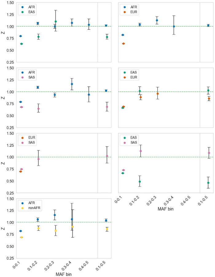
Fig 2 — The value of Z is plotted against the frequency of shared and private polymorphisms, for pairs of populations: AFR, EAS, EUR, and SAS. In each panel, we show the value of Z for a comparison of 2 populations using the private polymorphisms from each, the population used being indicated in the plot legend. Data binned by minor allele frequency bins of size 0.1 on the x-axis. The final bin is 0.1–0.5 (i.e., all data minus the lowest frequency bin). Only data points in which there were at least 20 polymorphisms for all polymorphism categories were plotted, because the confidence intervals were very large otherwise. Code to extract and analyse the data can be found at https://github.com/vivaksoni/test_for_balancing_selection. The data underlying this figure can be found in S3 Data. AFR, Africans; EAS, East Asians; EUR, Europeans; SAS, South Asians.

If we estimate α_b in those comparisons in which Z is significantly greater than 1, we estimate that approximately 2% to 4% of the nonsynonymous shared polymorphisms between the African and other human populations are subject to balancing selection (Table 1). These estimates are likely to be underestimates because there will still be SDMs segregating in our data, even though we have removed the lowest frequency variants (see simulation results). The proportions suggest that at least 200 to 400 polymorphisms, which are shared between the African and other populations, are maintained by balancing selection (Table 1).

Table 1. The level of balancing selection in humans.

Estimates of the proportion of shared nonsynonymous polymorphisms under balancing selection, α_b, and the number of polymorphisms, b, being directly maintained by balancing selection for population comparisons in which Z > 1. Code to extract and analyse the data can be found at https://github.com/vivaksoni/test_for_balancing_selection.

Target population	Comparative population	α_b	α_{b_low}	α_{b_high}	b	b_low	b_high
African	Non-African	0.0407	0.0123	0.0671	366	111	604
African	European	0.0400	0.0100	0.0600	577	176	926
African	East Asian	0.0174	0.0003	0.0351	223	4	451
African	South Asian	0.0251	0.0064	0.0439	341	87	595

Open in a new tab

A concern in any analysis of human population genetic data is the influence of biased gene conversion (BGC). This process tends to increase the number and allele frequencies of AT > GC mutations, and reduce the number and allele frequencies of GC > AT mutations. If this process differentially affects synonymous and nonsynonymous sites and shared and private polymorphisms, then it could potentially lead to Z > 1. To investigate whether BGC has an effect, we performed 2 analyses. In the first, we divided our genes according to whether they were in high and low recombining regions, dividing the data at the median recombination rate (RR). Our 2 groups differ substantially in their mean rate of recombination (mean RR in low group = 1.2 × 10^‒7 centimorgans per site and high group = 1.8 × 10^‒6 centimorgans per site). We find that Z is actually higher in the low RR regions, although not significantly so (Table 2). However, neither estimate of Z is significantly greater than 1.

Table 2. Testing for the influence of biased gene conversion I.

Estimates of Z for data split by median recombination rate. Code to extract and analyse the data can be found at https://github.com/vivaksoni/test_for_balancing_selection.

Mean recombination rate	Z	Z_low	Z_high
1.20 × 10^‒9	1.02	0.99	1.06
1.80 × 10^‒8	1.00	0.96	1.04

Open in a new tab

In the second test of the influence of BGC on the value of Z, we limited our analysis to mutations that are not affected by BGC—i.e., G<>C and A<>T mutations. This reduces our dataset by about 80%. As a consequence, we summed the data for all polymorphisms with frequencies >0.1. We find that our estimates are largely unchanged compared to when all polymorphisms are included, except in the case of the African-East Asian comparison; however, the confidence intervals are increased substantially so that Z is not significantly greater than 1 for any comparison (Table 3). Our 2 tests are inconclusive; in both cases, our values of Z are largely unaffected, but the reduction in sample size increases the variance of our estimate and all estimates become nonsignificant.

Table 3. Testing for the effects of biased gene conversion II.

The values of Z when only G<>C and A<>T mutations are considered. Code to extract and analyse the data can be found at https://github.com/vivaksoni/test_for_balancing_selection.

Target population	Comparative population	All polymorphism data			Filtered for BGC
Target population	Comparative population	Z	Z_low	Z_high	Z	Z_low	Z_high
African	Non-African	1.04	1.01	1.07	1.03	0.94	1.12
African	East Asian	1.02	1.00	1.04	0.96	0.91	1.02
African	South Asian	1.03	1.01	1.05	1.02	0.96	1.08

Open in a new tab

BGC, biased gene conversion.

Groups of genes

We can potentially apply our test of balancing selection to individual genes or groups of genes, where we have enough data. Balancing selection has been implicated in the evolution of immune-related genes (e.g., [4,15,23,24]), particularly major histocompatibility complex (MHC) or human leukocyte antigen (HLA) genes [25,26]. To investigate whether we could detect this signature in our data, we split our dataset into HLA and non-HLA genes [27]. Due to a lack of private polymorphisms, we combined all frequency categories >0.1. We find that Z > 1 for HLA genes in those population comparisons in which Z > 1 overall and in most cases this pattern is significant. We estimate that a very substantial proportion of nonsynonymous genetic variation is being maintained by balancing selection, although the confidence intervals on our estimates are large; roughly 50% of the shared nonsynonymous SNPs are being maintained by balancing selection between African and non-African populations in the HLA region and this equates to approximately 200 polymorphisms (Table 4). If we consider non-HLA genes, we find that Z > 1; however, the values are never significant and the estimated proportion of shared polymorphisms that are being maintained by balancing selection is very low (Table 5).

Table 4. Balancing selection in HLA genes.

Estimates of the proportion of shared nonsynonymous polymorphisms under balancing selection, α_b, and the number of polymorphisms being directly maintained by balancing selection, b, for population comparisons in the HLA region for population comparisons in which Z > 1 when using all genes. Estimates for polymorphisms with frequency >0.1. Missing values indicate the lower confidence interval was less than 1. Data consist of 177 genes. Code to extract and analyse the data can be found at https://github.com/vivaksoni/test_for_balancing_selection.

Target	Comparative	α	α_{b_low}	α_{b_low}	b	b _low	b _high
AFR	Non-AFR	0.70	0.19	0.79	208	56	233
AFR	EAS	0.28	-	0.46	131	-	213
AFR	SAS	0.54	0.28	0.69	253	129	323

Open in a new tab

AFR, Africans; EAS, East Asians; HLA, human leukocyte antigen; SAS, South Asians.

Table 5. Balancing selection in non-HLA genes.

Estimates of the proportion of shared nonsynonymous polymorphisms under balancing selection, α_b, in non-HLA genes, and the number of polymorphisms being directly maintained by balancing selection, b, for population comparisons in which Z > 1 when using all genes. Missing values indicate the lower confidence interval was less than 1. Data consist of 19,212 genes. Code to extract and analyse the data can be found at https://github.com/vivaksoni/test_for_balancing_selection.

Target	Comparative	α_b	α_{b_low}	α_{b_high}	b	b _low	b _high
AFR	Non-AFR	0.024	-	0.050	207	-	433
AFR	EAS	0.002	-	0.020	21	-	245
AFR	SAS	0.009	-	0.025	120	-	332

Open in a new tab

AFR, Africans; EAS, East Asians; HLA, human leukocyte antigen; SAS, South Asians.

If we run our analysis grouping genes by their Gene Ontology (GO) category and restricting the analysis to those groups that have at least 100 polymorphisms with frequencies >0.1, we find 606 categories in which Z is significantly greater than 1 in at least 1 population comparison comparing all pairs of populations (S1 Fig). We list those significant in 5 or more population comparisons in Table 6. One of these GO categories, “endoplasmic reticulum membrane” is shared across 6 of the 14 population comparisons; among those categories shared among 5 are “viral process” and “response to stimulus.” Fifty-four categories are shared between 4 or more population comparisons, and 108 among 3 or more population comparisons. These include 6 categories related to immunity (including immune system process which is significant in 5 population comparisons), and 40 categories that are linked to antigen presentation though not classified as immune-related categories. There are also 2 viral-related categories (including viral process which is significant in 5 population comparisons).

Table 6. GO category analysis.

GO categories in which Z is significantly greater than 1 in at least 5 population comparisons. Code to extract and analyse the data can be found at https://github.com/vivaksoni/test_for_balancing_selection.

GO category	Counts
Endoplasmic reticulum membrane	6
Nucleic acid binding	5
Viral process	5
Response to stimulus	5
Intermediate filament	5
Zinc ion binding	5
Chromatin binding	5
Chromosome	5

Open in a new tab

Individual genes

Although our test is likely to have little power for individual genes (see above), we applied our statistic, combining all frequency bins (0 to 0.5) due to a lack of polymorphism data. We tested for significance using a 1-tailed Fisher’s exact test. Of the 14,261 genes, we analysed 514 had Z > 1 in at least 1 population comparison. Eighteen of these were nominally significant at p < 0.1 (S2 Data), but no gene was individually significant when we corrected for multiple testing using a Bonferroni correction. Eighteen genes have Z > 1 in at least 9 population comparisons; note that since populations share polymorphisms, we cannot combine the evidence for balancing selection across these populations (Table 7). Four of these genes, MUC4, RP1L1, PKD1L2, and ZAN, have Z > 1 in all population comparisons.

Table 7. Single gene analysis.

Genes with Z > 1 in multiple population comparisons. Code to extract and analyse the data can be found at https://github.com/vivaksoni/test_for_balancing_selection.

Gene symbol	Number of population comparisons in which Z > 1
MUC4	14
RP1L1	14
PKD1L2	14
ZAN	14
C1orf167	13
SPTBN5	12
MKI67	12
DNAH14	11
WDFY4	10
FAM230G	10
CMYA5	9
CRIPAK	9
SYNE2	9
FSIP2	9
GREB1	9
ALMS1	9
MUC19	9
CENPF	9

Open in a new tab

If we use the 514 genes and do a GO enrichment analysis, we find multiple GO categories enriched for these genes including immune response categories with 3-fold enrichment. The most highly enriched categories are involved in energy production and conversion (including dynein binding) and intracellular transport (including microtubule motor activity) (S2 Data).

Discussion

We propose a new method for detecting and quantifying the amount of balancing selection that is operating on polymorphisms, in which the numbers of nonsynonymous and synonymous polymorphisms that are shared between populations and species are compared to those that are private. The method is analogous to the McDonald–Kreitman test used to test and quantify the amount of adaptive evolution between species [16]. Our method is simple to apply and yields an estimate of the number of polymorphisms directly subject to balancing selection, as opposed to those affected by linkage. We show that our test is robust to the presence of SDMs under simple demographic models of population division, expansion, and migration. When we apply our method to data from human populations, we find evidence that hundreds of nonsynonymous polymorphisms are probably being maintained by balancing selection in human populations. However, most of this signal comes from the HLA region.

Our method for detecting balancing selection appears to be robust to changes in demography. The classic MK test of adaptive evolution between species can generate artefactual evidence of adaptive evolution if there are SDMs and there has been population size expansion [16,28]; this is because SDMs that might have been fixed when the effective population size was small, no longer segregate once the population size is large. A similar bias does not appear to affect our test, although we have only investigated 2 DFEs and a limited number of demographic scenarios. Our test is likely to be more robust than the classic MK test because the shared polymorphisms are affected by the demographic changes that affect the private polymorphisms, i.e., if the population expands this will increase the effectiveness of natural selection on both the private and the shared polymorphisms. However, although our method seems to be relatively robust to changes in demography, in the sense that it does not generate artefactual evidence of balancing selection, it is evident that demography does affect the chance of balancing selection being identified, because the values of Z depend on the demography and which population the private polymorphisms are taken from (Fig 2). Furthermore, the method generally underestimates the number of balanced polymorphisms.

The method can in principle be applied to any pair of populations or species. However, the test is likely to be weak when the populations/species are closely related for 2 reasons. First, there will be relatively few private polymorphisms, and second, the proportion of shared polymorphisms that are subject to balancing selection is likely to be low, because so many neutral polymorphisms are shared between populations because of recent common ancestry. As the populations/species diverge so the number of private polymorphisms will increase, and the proportion of shared polymorphisms that are balanced will increase. Of course, as the time of divergence increases so the selective conditions that maintained the polymorphism are likely to change and the polymorphism might become neutral or subject to directional selection.

Our method is also likely, like all methods, to be better at detecting balanced polymorphisms that are common, because most populations are dominated by large numbers of rare neutral variants. The method requires that the neutral and selected sites are interdigitated; the method is therefore easy to apply to protein coding sequences, but may be more difficult to apply to other types of variation, such as that which affects gene expression. The method is weakly powered to detect balancing selection in individual genes (S34 and S35 Figs). Most other methods or analyses have leveraged patterns of variation in LD with a balanced polymorphism [6–15]; such variation obscures the signal that our method detects, which is an excess of shared variation.

The great advantage of our method is that it gives an estimate of the proportion and number of shared polymorphisms that are directly subject to balancing selection, under a set of simplifying assumptions, and it is simple to apply. However, the method is likely to yield underestimates of the proportion of balanced polymorphisms, under more realistic models of evolution, something we have confirmed by simulation (S16–S33 Figs). We have assumed, in deriving α_b, that all nonsynonymous mutations are either strongly deleterious, neutral, or subject to balancing selection. However, a substantial fraction of nonsynonymous mutations appear to be slightly deleterious in humans [19,29–32] and other species [19,30,33,34]—i.e., they are deleterious, but sufficiently weakly selected that they contribute to polymorphism. Under stationary population size assumptions—i.e., in which the ancestral population is duplicated to form the daughter populations—this will lead to an underestimate of α_b because SDMs tend to contribute more to private than shared polymorphism, and hence inflate R_N/R_S relative to S_N/S_S (Fig 1). Under more realistic demographic models, in which at least one of the derived populations is reduced, this is expected to depress α_b in the population that is being reduced because more SDMs will tend to segregate in smaller populations, hence inflating R_N/R_S (compare Fig 2 and S3 Fig).

The second reason that we are likely underestimating the number of balanced polymorphisms using our simple method is that we assume that there are no balanced polymorphisms that are private to each population; these would inflate R_N/R_S. Private balanced polymorphisms might arise from an ancestral polymorphism that is lost from 1 of the daughter populations or 1 that arises de novo. A more realistic model of balancing selection is one in which balanced polymorphisms are continually generated with the selective forces persisting for some time before they dissipate [35] and the balanced polymorphism is lost. The process of population division itself is likely to lead to the loss of many balanced polymorphisms as the environment shifts in the 2 daughter populations.

A potential solution to the tendency for our method to underestimate Z and α_b is to simulate data under a realistic demographic model both with and without balancing selection, and use the simulations to estimate the proportion of balanced polymorphisms. However, there are challenges in this approach; in particular, we need an accurate demographic model. We have performed simulations under the commonly used human demographic model inferred by Gravel and colleagues [36] estimating the DFE from the current African population, assuming no balancing selection; we chose the African population because it has been subject to relatively modest demographic change. Our observed Z values do not match the simulated values (S36 Fig); in particular, we find that the observed values of Z are substantially greater than the simulated among the low frequency polymorphisms. However, the model of Gravel and colleagues does not fit the site frequency spectrum (SFS) of the individual populations of 1,000 genome data; for example, in the African population there are far too many singleton SNPs even among the putative neutral synonymous mutations (S37 Fig). The lack of fit is perhaps not surprising; Gravel and colleagues inferred their model using 80 chromosomes per population, whereas the 1,000 genome data contain >1,000 chromosomes per population. Furthermore, the inference of a demographic model should take into account the influence of BGC and background selection, which appear to be pervasive factors in the human genome [37], so these simulations will be complex.

We have analysed data from human populations and find some evidence for widespread balancing selection, particularly using private polymorphisms from the African population. It might be argued that detecting a signal of balancing selection using the private polymorphisms from 1 population is weak evidence of balancing selection. However, simulations suggest that this is likely to be common under many demographic models (S1–S15 Figs) when there are modest levels of balancing selection.

Controlling for BGC in our data analysis leads to inconclusive results; our estimates are not greatly affected by BGC, but because of the reduction in the sample size the confidence intervals increase and our estimates are not significantly different from zero. Much of the signal for balancing selection comes from the HLA genes. However, an analysis of GO categories suggests that numerous categories show evidence of balancing selection across multiple population comparisons (S1 Data). Some of these are expected, but many are not, such as “nucleic acid binding,” which is significant in 5 of the 14 population comparisons (12 population comparisons plus African–non-African).

No individual gene is significant when we control for multiple testing; however, several genes have Z > 1 in multiple population comparisons including 10 that are shared across at least 10 of the 14 population comparisons. Three of these overlap with previous genome-wide scans of selection, namely the protein-coding gene DNAH14, implicated in brain compression and encoding axonemal dynein [38]; MUC4, implicated in biliary tract cancer [39]; and ZAN, which encodes a protein involved in sperm adhesion, previously implicated in balancing selection and positive selection in human populations [40]. Two of these 10 genes are associated with tumours. MKI67 expression is associated with a higher tumour grade and early disease recurrence [41], and WDFY4 plays a critical role in the regulation of certain viral and tumour antigens in dendritic cells [42]. PKD1L2 is associated with polycystic kidney disease, and RP1L1 variants are associated with several retinal diseases including occult macular dystrophy [43]. SPTBN5 encodes for the cytoskeletal protein spectrin that plays a role in maintaining cytoskeletal structure [44], and C1orf167 expresses open reading frame protein that is highly expressed in the testis [45]. Finally, FAM230G is highly expressed in testes [46].

Twenty-five of the 514 genes with Z > 1 overlap with those genes identified by Bitarello and colleagues [15], but this is similar to the level of overlap expected at random, i.e., they observed that 7.9% of protein coding genes overlapped regions identified by their method as being subject to balancing selection, and we identified 514 candidates, so we expect 0.079 × 514 = 41 by chance alone. The lack of a significant overlap is possibly not surprising; we have applied our method to nonsynonymous variation, whereas the method of Bitarello and colleagues [15] considers all variation. Furthermore, the method of Bitarello and colleagues [15] is most powerful at detecting balancing selection over long time periods; in the case of humans, over periods of millions of years. In contrast, we have applied our method to populations that diverged 10,000s of years ago.

A signature of overdominance or heterozygous advantage can be produced by linkage to recessive or partially recessive deleterious mutations. For example, let us imagine that we have 2 closely linked loci at which we have deleterious alleles; let the A2 allele be the recessive allele at the A locus and the B2 allele at the B locus. Now consider a third neutral locus with alleles C1 and C2. If C1 is in LD with the A2 allele, and C2 is in LD with the B2 allele, then C1C2 heterozygous individuals will have higher fitness than C1C1 and C2C2 homozygotes. This form of selection is known as associative overdominance and can lead to the maintenance of genetic variation [47] in low RR regions. However, there is no reason why nonsynonymous mutations should be linked to other deleterious recessives more frequently than synonymous mutations, and Z is not substantially greater in regions of low recombination, so associative overdominance seems an unlikely explanation for our results (Table 2).

Conclusion

We present a new approach to test for the presence of balancing selection and to the number of polymorphisms that are directly affected by it. Our method appears to be robust to demographic change. Application of the method to human population genetic data suggests that 100s of nonsynonymous polymorphisms shared between populations might be maintained by balancing selection.

Methods and materials

Human data

Human variation data were obtained from 1,000 genomes Grch37 vcf files [22]. Variants were annotated using Annovar’s hg19 database [48]. The annotated data were then parsed to remove multinucleotide polymorphisms and indels. Because 1,000 genomes data provide allele frequencies for the non-reference allele rather than the minor allele, the minor allele frequency for each superpopulation and also for the global minor allele frequency was calculated. We used 1,000 genomes from the African, South Asian, East Asian, and European populations. The American population was removed due to the fact that it is an admixed population. GO category information was obtained from Ensembl’s BioMart data mining tool [18]. We used pyrho demography-aware recombination rate maps [49] for analyses that control for recombination rate.

Data analysis

We calculated our test statistic Z for each pair of human populations, and also for the comparison between African and non-African data separating polymorphisms by frequency into bins of 0.1. We do not attempt to orient SNPs but use the folded site frequency spectrum. This is because there are potential difficulties with inferring the ancestral state when some sites such as CpG dinucleotides have rates of mutation; this is compounded by the fact that there is substantial variation in the mutation rate that is not associated with sequence context [50] and is therefore difficult to control for; as a consequence, a fraction of high frequency variants may simply be due to misinference. The folded site frequency spectrum does not suffer from these problems. We take the frequency of the shared polymorphism to be the frequency in the population from which the private polymorphisms are drawn. To test for statistical significance, we summed the values of S_N, S_S, R_N, and R_S across genes and bootstrapped the data by gene 100 times to derive the 95% confidence intervals and standard error.

Simulations

All simulations were run using the SLiM 3.1 [51]. Parameter values were taken from human estimates. Almost all simulations were of a 288 bp locus, this being the average size of a human exon [18]. Unless otherwise stated, the scaled recombination rate and scaled mutation rate were set at r = 1.1 × 10^‒8 [52], μ = 2.5 × 10^‒8 [53] in the ancestral population. The distribution of fitness effects was assumed to be a gamma distribution, and the shape and mean strength of selection estimates for humans were taken from Eyre-Walker and colleagues [17] (shape parameter β = 0.23; mean N_es = 425). For Drosophila, estimates were taken from Keightley and Eyre-Walker [54] (β = 0.35; mean N_es = 1,800); again these were values in the ancestral population. Unless dominance was fixed, it was calculated using the model of Huber and colleagues [55], which was estimated from Arabidopsis species. The Huber model varies the dominance coefficient depending on the selection coefficient of the mutation, where the dominance coefficient increases with the strength of selection. Its formula is $h = f (s) = \frac{1}{\frac{1}{θ_{i n t e r c e p t}} - θ_{r a t e} s}$ , where θ_intercept defines the values of h at s = 0, and θ_rate determines how quickly h approaches 0 with decreasing negative selection coefficient. We set θ_intercept to 0.5 so that all mutations with a selection coefficient of s = 0 have a dominance coefficient, h = 0.5, and θ_rate = 41225.56. This assumes an inverse relationship between h and s, which gives the highest log likelihood score of the relationships compared by Huber and colleagues [55]. For balancing selection simulations, we assume a model of negative frequency-dependent selection; the equilibrium frequency was sampled from a uniform distribution between 0 and 1, with the Ns value at equilibrium set to 20, where N is the ancestral population size (see recipe 10.4.1 in SLiM [51] for details on how this was coded); however, it should be noted that some balanced polymorphisms with low equilibrium frequencies were lost in one of the descendent populations, so the realised distribution of frequencies is biased towards common polymorphisms (S38 Fig). Simulations in which the balanced polymorphism was lost from one of the 2 populations were discarded. The balanced polymorphism is introduced at the centre of the 288-bp region. Two million simulation runs were conducted for each model. This reduced the standard error on our estimates of Z to very low levels.

For the generic simulations (i.e., not those involving the human demographic model), the ancestral population size was set at 200. This was allowed to equilibrate for 15 N generations before a balanced polymorphism was introduced 5 N generations before the population was split into 2. The descendant populations were then sampled every 0.05 N generations up to 20 N generations after the split. We ran 5 different generic simulations: (i) simulations in which the ancestral population was duplicated; (ii) vicariance simulations in which the ancestral population was divided between the daughter populations in splits of 0.5 N to 0.5 N, 0.75 N to 0.25 N, 0.9 N to 0.1 N; (iii) variance simulations in which the descendant populations expanded; (iv) dispersal simulations, in which some variable fraction (0.5 N, 0.25 N, 0.1 N) of the ancestral population is duplicated to form the dispersal population, and the ancestral population continues as the other daughter population; and (v) dispersal with population increase of the dispersal population. The dispersal population starts as 0.1 N and expands exponentially 2 to 10× its original size after 21 N generations. Scenarios (ii) to (v) were repeated with migration rates of 0.01 N and 0.001 N of the ancestral population size between the descendant populations.

To investigate the power of the method to detect balancing selection in single genes, we ran a series of simulations of a single human gene; on average human genes are 32 kb in length, with an average exon size of 288 bp [18], 8.8 exons per gene, and 7.8 introns [56]. We simulated 9 exons of length 288 bp separated by 8 introns of 5,419 bp [56]. These loci were subject to human levels of mutation and recombination. We also ran a series of simulations of a gene that was 10-fold larger, in terms of the number of introns and exons. We ran simulations in which all mutations were deleterious and drawn from a gamma distribution, and a series of simulations in which a balanced polymorphism was introduced in the centre of each exon 5 N generations before the population was divided into 2 equal size populations (half the original population size). We only kept those balancing selection simulations in which at least 1 balance polymorphism survived to the sampling time point in both populations. In these simulations, we calculated Z using polymorphisms at all frequencies.

We also ran some simulations under the human demographic model of Gravel and colleagues [36]. The distribution of fitness effects for deleterious mutations was assumed to be a gamma distribution using the parameters estimated from the African superpopulation using the GammaZero model within the Grapes software [57]; the parameters are similar to those estimated by Eyre-Walker and colleagues [17], and used in the generic simulations (gamma shape = 0.17 and mean N_es = 1144). We chose to infer the DFE for the African superpopulation because this is currently the largest dataset available for a population that has been inferred to be relatively stable. Dominance was calculated using the Huber model discussed above. Sampling of all populations (African, East Asian, and European) was conducted at the end of the simulation (i.e., the equivalent of the present day). Each simulation was run 2 million times.

Supporting information

S1 Data. GO categories for which Z is significantly greater than 1, for each of the population comparisons.

(XLSX)

Click here for additional data file.^{(162KB, xlsx)}

S2 Data. Individual genes for which Z > 1, for each of the population comparisons.

(XLSX)

Click here for additional data file.^{(117.2KB, xlsx)}

S3 Data. Data underlying Fig 2 and S36–S38 Figs.

(XLSX)

Click here for additional data file.^{(34.4KB, xlsx)}

S1 Fig. Vicariance simulations, with human DFE, in which the ancestral population splits to form 2 daughter populations of the size specified in the panel.

Each column is a separate set of simulations, with the top row plotting Z against tMRCA (measured in N generations, where N is the population size) for the larger daughter population, and the bottom row the smaller. There is no balancing selection and deleterious mutations are drawn from a gamma DFE with parameters inferred from human population data. Code to run these simulations can be found at https://github.com/vivaksoni/test_for_balancing_selection. DFE, distributions of fitness effect; tMRCA, time to the most recent common ancestor.

(TIF)

Click here for additional data file.^{(55.2KB, tif)}

S2 Fig. Dispersal simulations, with human DFE, in which a single daughter population disperses from the ancestral population.

Each column is a separate set of simulations, with the top row plotting Z against tMRCA (measured in N generations, where N is the population size) for the ancestral population, and the bottom row the daughter population. There is no balancing selection and deleterious mutations are drawn from a gamma DFE with parameters inferred from human population data. Code to run these simulations can be found at https://github.com/vivaksoni/test_for_balancing_selection. DFE, distributions of fitness effect; tMRCA, time to the most recent common ancestor.

(TIF)

Click here for additional data file.^{(54KB, tif)}

S3 Fig. Vicariance and expansion simulations, with human DFE, in which both daughter populations expand.

The ancestral population (of size N = 200) splits to form 2 daughter populations of size N = 100. Both daughter populations go on to expand in size. In the left column, the daughter populations double in size. In the right panel, they reach 10× their initial size. There is no balancing selection and deleterious mutations are drawn from a gamma DFE with parameters inferred from human population data. Code to run these simulations can be found at https://github.com/vivaksoni/test_for_balancing_selection. DFE, distributions of fitness effect; tMRCA, time to the most recent common ancestor.

(TIF)

Click here for additional data file.^{(40.6KB, tif)}

S4 Fig. Vicariance and expansion simulations, with human DFE, in which only 1 daughter population expands.

The ancestral population (of size N = 200) splits to form 2 daughter populations of size N = 100. One daughter population (upper panels) goes on to expand in size. In the left column, the daughter populations double in size. In the right panel, they reach 10× their initial size. There is no balancing selection and deleterious mutations are drawn from a gamma DFE with parameters inferred from human population data. Code to run these simulations can be found at https://github.com/vivaksoni/test_for_balancing_selection. DFE, distributions of fitness effect; tMRCA, time to the most recent common ancestor.

(TIF)

Click here for additional data file.^{(42.4KB, tif)}

S5 Fig. Dispersal and expansion simulations, with human DFE, in which a single daughter population disperses from the ancestral population and then expands.

The ancestral population (of size N = 200) splits to form a daughter population of size N = 100, which expands to the final population size shown in the panel. Each column is a separate set of simulations, with the top row plotting Z against tMRCA (measured in N generations, where N is the population size) for the ancestral population, and the bottom row the daughter population. There is no balancing selection and deleterious mutations are drawn from a gamma DFE with parameters inferred from human population data. Code to run these simulations can be found at https://github.com/vivaksoni/test_for_balancing_selection. DFE, distributions of fitness effect; tMRCA, time to the most recent common ancestor.

(TIF)

Click here for additional data file.^{(54.5KB, tif)}

S6 Fig. Vicariance simulations, with Drosophila DFE, in which the ancestral population splits to form 2 daughter populations of the size specified in the panel.

Each column is a separate set of simulations, with the top row plotting Z against tMRCA (measured in N generations, where N is the population size) for the larger daughter population, and the bottom row the smaller. There is no balancing selection and deleterious mutations are drawn from a gamma DFE with parameters inferred from D. melanogaster population data. Code to run these simulations can be found at https://github.com/vivaksoni/test_for_balancing_selection. DFE, distributions of fitness effect; tMRCA, time to the most recent common ancestor.

(TIF)

Click here for additional data file.^{(51.2KB, tif)}

S7 Fig. Dispersal simulations, with Drosophila DFE, in which a single daughter population disperses from the ancestral population.

Each column is a separate set of simulations, with the top row plotting Z against tMRCA (measured in N generations, where N is the population size) for the ancestral population, and the bottom row the daughter population. There is no balancing selection and deleterious mutations are drawn from a gamma DFE with parameters inferred from D. melanogaster population data. Code to run these simulations can be found at https://github.com/vivaksoni/test_for_balancing_selection. DFE, distributions of fitness effect; tMRCA, time to the most recent common ancestor.

(TIF)

Click here for additional data file.^{(55KB, tif)}

S8 Fig. Vicariance expansion simulations, with Drosophila DFE, in which both daughter populations expand.

The ancestral population (of size N = 200) splits to form 2 daughter populations of size N = 100. Both daughter populations go on to expand in size. In the left column, the daughter populations double in size. In the right panel, they reach 10× their initial size. There is no balancing selection and deleterious mutations are drawn from a gamma DFE with parameters inferred from D. melanogaster population data. Code to run these simulations can be found at https://github.com/vivaksoni/test_for_balancing_selection. DFE, distributions of fitness effect; tMRCA, time to the most recent common ancestor.

(TIF)

Click here for additional data file.^{(41.7KB, tif)}

S9 Fig. Vicariance expansion simulations, with Drosophila DFE, in which only 1 daughter population expands.

The ancestral population (of size N = 200) splits to form 2 daughter populations of size N = 100. One daughter population (upper panels) goes on to expand in size. In the left column, the daughter populations double in size. In the right panel, they reach 10× their initial size. There is no balancing selection and deleterious mutations are drawn from a gamma DFE with parameters inferred from D. melanogaster population data. Code to run these simulations can be found at https://github.com/vivaksoni/test_for_balancing_selection. DFE, distributions of fitness effect; tMRCA, time to the most recent common ancestor.

(TIF)

Click here for additional data file.^{(43.9KB, tif)}

S10 Fig. Dispersal expansion simulations, with Drosophila DFE, in which a single daughter population disperses from the ancestral population and then expands.

The ancestral population (of size N = 200) splits to form a daughter population of size N = 100, which expands to the final population size shown in the panel. Each column is a separate set of simulations, with the top row plotting Z against tMRCA (measured in N generations, where N is the population size) for the ancestral population, and the bottom row the daughter population. There is no balancing selection and deleterious mutations are drawn from a gamma DFE with parameters inferred from D. melanogaster population data. Code to run these simulations can be found at https://github.com/vivaksoni/test_for_balancing_selection. DFE, distributions of fitness effect; tMRCA, time to the most recent common ancestor.

(TIF)

Click here for additional data file.^{(57.8KB, tif)}

S11 Fig. Vicariance simulations with migration and human DFE, in which the ancestral population splits to form 2 daughter populations of the size specified in the panel.

Each column is a separate set of simulations, with the top row plotting Z against tMRCA (measured in N generations, where N is the population size) for the larger daughter population, and the bottom row the smaller. There is no balancing selection and deleterious mutations are drawn from a gamma DFE with parameters inferred from human population data. Migration rate is 0.01 N. Code to run these simulations can be found at https://github.com/vivaksoni/test_for_balancing_selection. DFE, distributions of fitness effect; tMRCA, time to the most recent common ancestor.

(TIF)

Click here for additional data file.^{(55.6KB, tif)}

S12 Fig. Dispersal simulations with migration and human DFE, in which a single daughter population disperses from the ancestral population.

Each column is a separate set of simulations, with the top row plotting Z against tMRCA (measured in N generations, where N is the population size) for the ancestral population, and the bottom row the daughter population. There is no balancing selection and deleterious mutations are drawn from a gamma DFE with parameters inferred from human population data. Migration rate is 0.01 N. Code to run these simulations can be found at https://github.com/vivaksoni/test_for_balancing_selection. DFE, distributions of fitness effect; tMRCA, time to the most recent common ancestor.

(TIF)

Click here for additional data file.^{(59.7KB, tif)}

S13 Fig. Dispersal expansion simulations with migration and human DFE, in which a single daughter population disperses from the ancestral population and then expands.

The ancestral population (of size N = 200) splits to form a daughter population of size N = 100, which expands to the final population size shown in the panel. Each column is a separate set of simulations, with the top row plotting Z against tMRCA (measured in N generations, where N is the population size) for the ancestral population, and the bottom row the daughter population. There is no balancing selection and deleterious mutations are drawn from a gamma DFE with parameters inferred from human population data. Migration rate is 0.01 N. Code to run these simulations can be found at https://github.com/vivaksoni/test_for_balancing_selection. DFE, distributions of fitness effect; tMRCA, time to the most recent common ancestor.

(TIF)

Click here for additional data file.^{(59KB, tif)}

S14 Fig. Simulations, with human DFE, for combined 0.1–0.5 minor allele frequencies.

Each panel is a separate simulated scenario, with population sizes listed in the panel legend. (*) indicates simulations with migration (with migration rate 0.01 N). The first number is for the filled in data lines, denoting the ancestral population in dispersal scenarios, and for the larger population in the vicariance scenarios. The second number is for the dotted data lines, denoting the daughter population in dispersal scenarios, and the smaller population in the vicariance scenarios. For more details on each scenario, please see S1–S10 Figs. There is no balancing selection and deleterious mutations are drawn from a gamma DFE with parameters inferred from human population data. Code to run these simulations can be found at https://github.com/vivaksoni/test_for_balancing_selection. DFE, distributions of fitness effect; tMRCA, time to the most recent common ancestor.

(TIF)

Click here for additional data file.^{(190.7KB, tif)}

S15 Fig. Simulations, with Drosophila DFE, for combined 0.1–0.5 minor allele frequencies.

Each panel is a separate simulated scenario, with population sizes listed in the panel legend. (*) indicates simulations with migration (with migration rate 0.01 N). The first number is for the filled in data lines, denoting the ancestral population in dispersal scenarios, and for the larger population in the vicariance scenarios. The second number is for the dotted data lines, denoting the daughter population in dispersal scenarios, and the smaller population in the vicariance scenarios. For more details on each scenario, please see Supporting information S1–S10 Figs. There is no balancing selection and deleterious mutations are drawn from a gamma DFE with parameters inferred from D. melanogaster population data. Code to run these simulations can be found at https://github.com/vivaksoni/test_for_balancing_selection. DFE, distributions of fitness effect; tMRCA, time to the most recent common ancestor.

(TIF)

Click here for additional data file.^{(189.4KB, tif)}

S16 Fig. Comparison of α_{b inferred} and α_{b true} for dispersal simulation, sampled at 0.2 N generations after the population split, in which the ancestral population is of size N = 200, and the daughter population is size N = 20.

The top row plots are for the ancestral population, the bottom row for the daughter population. The left column plots α_{b inferred}/α_{b true} against the proportion of balancing selection simulations. The right column plots α_{b true} against the proportion of balancing selection simulations. The 0–0.1 MAF category has been removed, and negative values have been truncated to 0 for the sake of clarity. Deleterious mutations are drawn from a gamma DFE with parameters inferred from human population data. Code to run these simulations can be found at https://github.com/vivaksoni/test_for_balancing_selection. DFE, distributions of fitness effect; MAF, minor allele frequency.

(TIF)

Click here for additional data file.^{(65.3KB, tif)}

S17 Fig. Comparison of α_{b inferred} and α_{b true} for dispersal simulation, sampled at 1 N generations after the population split, in which the ancestral population is of size N = 200, and the daughter population is size N = 20.

(TIF)

Click here for additional data file.^{(48.3KB, tif)}

S18 Fig. Comparison of α_{b inferred} and α_{b true} for dispersal simulation, sampled at 0.2 N generations after the population split, in which the ancestral population is of size N = 200, and the daughter population is size N = 50.

(TIF)

Click here for additional data file.^{(64.7KB, tif)}

S19 Fig. Comparison of α_{b inferred} and α_{b true} for dispersal simulation, sampled at 1 N generations after the population split, in which the ancestral population is of size N = 200, and the daughter population is size N = 50.

(TIF)

Click here for additional data file.^{(58.6KB, tif)}

S20 Fig. Comparison of α_{b inferred} and α_{b true} for dispersal simulation, sampled at 0.2 N generations after the population split, in which the ancestral population is of size N = 200, and the daughter population is size N = 100.

(TIF)

Click here for additional data file.^{(64.1KB, tif)}

S21 Fig. Comparison of α_{b inferred} and α_{b true} for dispersal simulation, sampled at 1 N generations after the population split, in which the ancestral population is of size N = 200, and the daughter population is size N = 100.

(TIF)

Click here for additional data file.^{(66.5KB, tif)}

S22 Fig. Comparison of α_{b inferred} and α_{b true} for vicariance simulation, sampled at 0.2 N generations after the population split, in which the ancestral population is of size N = 200, and both daughter populations are size N = 100.

The top row plots are for 1 daughter population, the bottom row for the other. The left column plots α_{b inferred}/α_{b true} against the proportion of balancing selection simulations. The right column plots α_{b true} against the proportion of balancing selection simulations. The 0–0.1 MAF category has been removed, and negative values have been truncated to 0 for the sake of clarity. Deleterious mutations are drawn from a gamma DFE with parameters inferred from human population data. Code to run these simulations can be found at https://github.com/vivaksoni/test_for_balancing_selection. DFE, distributions of fitness effect; MAF, minor allele frequency.

(TIF)

Click here for additional data file.^{(63.9KB, tif)}

S23 Fig. Comparison of α_{b inferred} and α_{b true} for vicariance simulation, sampled at 1 N generations after the population split, in which the ancestral population is of size N = 200, and both daughter populations are size N = 100.

(TIF)

Click here for additional data file.^{(59.6KB, tif)}

S24 Fig. Comparison of α_{b inferred} and α_{b true} for vicariance simulation, sampled at 0.2 N generations after the population split, in which the ancestral population is of size N = 200, with 1 daughter population size N = 150 (top row) and the other size N = 50 (bottom row).

The left column plots α_{b inferred}/α_{b true} against the proportion of balancing selection simulations. The right column plots α_{b true} against the proportion of balancing selection simulations. The 0–0.1 MAF category has been removed, and negative values have been truncated to 0 for the sake of clarity. Deleterious mutations are drawn from a gamma DFE with parameters inferred from human population data. Code to run these simulations can be found at https://github.com/vivaksoni/test_for_balancing_selection. DFE, distributions of fitness effect; MAF, minor allele frequency.

(TIF)

Click here for additional data file.^{(63.5KB, tif)}

S25 Fig. Comparison of α_{b inferred} and α_{b true} for vicariance simulation, sampled at 1 N generations after the population split, in which the ancestral population is of size N = 200, with 1 daughter population size N = 150 (top row) and the other size N = 50 (bottom row).

(TIF)

Click here for additional data file.^{(57KB, tif)}

S26 Fig. Comparison of α_{b inferred} and α_{b true} for vicariance simulation, sampled at 0.2 N generations after the population split, in which the ancestral population is of size N = 200, with 1 daughter population size N = 180 (top row) and the other size N = 20 (bottom row).

(TIF)

Click here for additional data file.^{(63.6KB, tif)}

S27 Fig. Comparison of α_{b inferred} and α_{b true} for vicariance simulation, sampled at 1 N generations after the population split, in which the ancestral population is of size N = 200, with 1 daughter population size N = 180 (top row) and the other size N = 20 (bottom row).

(TIF)

Click here for additional data file.^{(46.5KB, tif)}

S28 Fig. Comparison of α_{b inferred} and α_{b true} for expansion simulation, sampled at 0.2 N generations after the population split, in which the ancestral population is of size N = 200, and the daughter population is size N = 40.

(TIF)

Click here for additional data file.^{(64.2KB, tif)}

S29 Fig. Comparison of α_{b inferred} and α_{b true} for expansion simulation, sampled at 1 N generations after the population split, in which the ancestral population is of size N = 200, and the daughter population is size N = 40.

(TIF)

Click here for additional data file.^{(46.9KB, tif)}

S30 Fig. Comparison of α_{b inferred} and α_{b true} for expansion simulation, sampled at 0.2 N generations after the population split, in which the ancestral population is of size N = 200, and the daughter population is size N = 400.

(TIF)

Click here for additional data file.^{(63.4KB, tif)}

S31 Fig. Comparison of α_{b inferred} and α_{b true} for expansion simulation, sampled at 1 N generations after the population split, in which the ancestral population is of size N = 200, and the daughter population is size N = 400.

(TIF)

Click here for additional data file.^{(56.4KB, tif)}

S32 Fig. Comparison of α_{b inferred} and α_{b true} for expansion simulation, sampled at 0.2 N generations after the population split, in which the ancestral population is of size N = 200, and the daughter population is size N = 2,430.

(TIF)

Click here for additional data file.^{(63.4KB, tif)}

S33 Fig. Comparison of α_{b inferred} and α_{b true} for expansion simulation, sampled at 1 N generations after the population split, in which the ancestral population is of size N = 200, and the daughter population is size N = 2,430.

(TIF)

Click here for additional data file.^{(64.1KB, tif)}

S34 Fig. The distribution of Z for simulations with (orange) and without (blue) balancing selection for a locus that has average human dimensions.

For each scenario 500,000 simulations were run. (*** p < 0.001 for a test between 2 distributions). Code to run these simulations can be found at https://github.com/vivaksoni/test_for_balancing_selection.

(TIF)

Click here for additional data file.^{(68.1KB, tif)}

S35 Fig. The distribution of Z for simulations with (orange) and without (blue) balancing selection for a locus that is 10-fold larger than the average human gene.

(TIF)

Click here for additional data file.^{(76.9KB, tif)}

S36 Fig. Simulations using the Gravel model of human demography (Gravel and colleagues, 2011).

Shown are the observed (filled circles) and simulated (crosses) values of Z. Each column represents a different population comparison. From left to right: AFR and EAS, AFR and EUR, EUR and EAS. The population name in the upper left indicates which set of private polymorphisms are used to calculate Z in each population comparison. The x-axis represents private polymorphism minor allele frequency bins. Confidence intervals generated by bootstrapping. Code to extract and analyse the data can be found at https://github.com/vivaksoni/test_for_balancing_selection. The data underlying this figure can be found in S3 Data. AFR, Africans; EAS, East Asians; EUR, Europeans.

(TIF)

Click here for additional data file.^{(44.3KB, tif)}

S37 Fig. Comparison of simulated (under the Gravel and colleagues (2011) model of human demography) and observed SFS from the African population.

The SFS is summarised by combining SNPs at counts of 2 and 3, 4 to 7, 8 to 15…etc. with singletons considered by themselves. Code to extract and analyse the data can be found at https://github.com/vivaksoni/test_for_balancing_selection. The data underlying this figure can be found in S3 Data.

(TIF)

Click here for additional data file.^{(26.6KB, tif)}

S38 Fig. Balanced polymorphisms were introduced under a model of frequency-dependent selection in which the equilibrium frequency was drawn from a uniform distribution.

However, rare polymorphisms are more likely to be lost; the figure shows the average minor allele frequency of shared balanced polymorphisms in a simulation in which the population was duplicated and sampled N generations after the duplication event. Code to run these simulations can be found at https://github.com/vivaksoni/test_for_balancing_selection. The data underlying this figure can be found in S3 Data.

(TIF)

Click here for additional data file.^{(125.2KB, tif)}

Abbreviations

BGC: biased gene conversion
DFE: distributions of fitness effect
GO: gene ontology
HLA: human leukocyte antigen
LD: linkage disequilibrium
MAF: minor allele frequency
MHC: major histocompatibility complex
RR: recombination rate
SDMs: slightly deleterious mutations
SFS: site frequency spectrum
tMRCA: time to most common recent ancestor

Data Availability

We have used the publicly available 1000 genome data available at https://www.internationalgenome.org.

Funding Statement

This research was supported by National Environment Research Council (NERC) grant NE/T008083/1 to author MV. URL: https://nerc.ukri.org/funding/next/publicationofwork/ The funders had no role in study design, data collection and analysis, decision to publish, or preparation of the manuscript.

References

1.Nielsen R. Molecular Signatures of Natural Selection. Annu Rev Genet. 2005;39(1):197–218. doi: 10.1146/annurev.genet.39.073003.112420 [DOI] [PubMed] [Google Scholar]
2.Allison AC. The sickle-cell and haemoglobin C genes in some African populations. Ann Hum Genet. 1956;21(1):67–89. [PubMed] [Google Scholar]
3.Nosil P, Villoutreix R, de Carvalho CF, Farkas TE, Soria-Carrasco V, Feder JL, et al. Natural selection and the predictability of evolution in Timema stick insects. Science. 2018;359(6377):765–70. doi: 10.1126/science.aap9125 [DOI] [PubMed] [Google Scholar]
4.Hughes AL, Nei M. Pattern of nucleotide substitution at major histocompatibility complex class I loci reveals overdominant selection. Nature. 1988;335(6186):167–70. doi: 10.1038/335167a0 [DOI] [PubMed] [Google Scholar]
5.Asthana S, Schmidt S, Sunyaev S. A limited role for balancing selection. Trends Genet. 2005;21(1):30–2. doi: 10.1016/j.tig.2004.11.001 [DOI] [PubMed] [Google Scholar]
6.Bubb KL, Bovee D, Buckley D, Haugen E, Kibukawa M, Paddock M, et al. Scan of Human Genome Reveals No New Loci Under Ancient Balancing Selection. Genetics. 2006;173(4):2165–77. doi: 10.1534/genetics.106.055715 [DOI] [PMC free article] [PubMed] [Google Scholar]
7.Andrés AM, Hubisz MJ, Indap A, Torgerson DG, Degenhardt JD, Boyko AR, et al. Targets of balancing selection in the human genome. Mol Biol Evol. 2009;26(12):2755–64. doi: 10.1093/molbev/msp190 [DOI] [PMC free article] [PubMed] [Google Scholar]
8.Leffler EM, Gao Z, Pfeifer S, Segurel L, Auton A, Venn O, et al. Multiple Instances of Ancient Balancing Selection Shared Between Humans and Chimpanzees. Science. 2013;339(6127):1578–82. doi: 10.1126/science.1234070 [DOI] [PMC free article] [PubMed] [Google Scholar]
9.DeGiorgio M, Lohmueller KE, Nielsen R. A Model-Based Approach for Identifying Signatures of Ancient Balancing Selection in Genetic Data. PLoS Genet. 2014;10(8):e1004561. doi: 10.1371/journal.pgen.1004561 [DOI] [PMC free article] [PubMed] [Google Scholar]
10.Gao Z, Przeworski M, Sella G. Footprints of ancient-balanced polymorphisms in genetic variation data from closely related species. Evolution. 2015;69(2):431–46. doi: 10.1111/evo.12567 [DOI] [PMC free article] [PubMed] [Google Scholar]
11.Hunter-Zinck H, Clark AG. Aberrant Time to Most Recent Common Ancestor as a Signature of Natural Selection. Mol Biol Evol. 2015;32(10):2784–97. doi: 10.1093/molbev/msv142 [DOI] [PMC free article] [PubMed] [Google Scholar]
12.Fijarczyk A, Babik W. Detecting balancing selection in genomes: limits and prospects. Mol Ecol. 2015;24(14):3529–45. doi: 10.1111/mec.13226 [DOI] [PubMed] [Google Scholar]
13.Sheehan S, Song YS. Deep Learning for Population Genetic Inference. PLoS Comput Biol. 2016;12(3):e1004845. doi: 10.1371/journal.pcbi.1004845 [DOI] [PMC free article] [PubMed] [Google Scholar]
14.Siewert KM, Voight BF. Detecting Long-Term Balancing Selection Using Allele Frequency Correlation. Mol Biol Evol. 2017;34(11):2996–3005. doi: 10.1093/molbev/msx209 [DOI] [PMC free article] [PubMed] [Google Scholar]
15.Bitarello BD, de Filippo C, Teixeira JC, Schmidt JM, Kleinert P, Meyer D, et al. Signatures of Long-Term Balancing Selection in Human Genomes. Genome Biol Evol. 2018;10(3):939–55. doi: 10.1093/gbe/evy054 [DOI] [PMC free article] [PubMed] [Google Scholar]
16.McDonald J, Kreitman M. Adaptive protein evolution at the Adh locus in Drosophila. Nature. 1991;351(6328):652–4. doi: 10.1038/351652a0 [DOI] [PubMed] [Google Scholar]
17.Eyre-Walker A, Woolfit M, Phelps T. The Distribution of Fitness Effects of New Deleterious Amino Acid Mutations in Humans. Genetics. 2006;173(2):891–900. doi: 10.1534/genetics.106.057570 [DOI] [PMC free article] [PubMed] [Google Scholar]
18.Yates A, Achuthan P, Akanni W, Allen J, Allen J, Alvarez-Jarreta J, et al. Ensembl 2020. Nucleic Acids Res. 2020;48(D1):D682–8. doi: 10.1093/nar/gkz966 [DOI] [PMC free article] [PubMed] [Google Scholar]
19.Fay JC, Wyckoff GJ, Wu CI. Positive and negative selection on the human genome. Genetics. 2001;158(3):1227–34. doi: 10.1093/genetics/158.3.1227 [DOI] [PMC free article] [PubMed] [Google Scholar]
20.Charlesworth J, Eyre-Walker A. The McDonald-Kreitman Test and Slightly Deleterious Mutations. Mol Biol Evol. 2008;25(6):1007–15. doi: 10.1093/molbev/msn005 [DOI] [PubMed] [Google Scholar]
21.Messer PW, Petrov DA. Frequent adaptation and the McDonald-Kreitman test. Proc Natl Acad Sci U S A. 2013;110(21):8615–20. doi: 10.1073/pnas.1220835110 [DOI] [PMC free article] [PubMed] [Google Scholar]
22.The 1000 Genomes Project Consortium. A global reference for human genetic variation. Nature. 2015;526(7571):68–74. doi: 10.1038/nature15393 [DOI] [PMC free article] [PubMed] [Google Scholar]
23.Weedall GD, Conway DJ. Detecting signatures of balancing selection to identify targets of anti-parasite immunity. Trends Parasitol. 2010;26(7):363–9. doi: 10.1016/j.pt.2010.04.002 [DOI] [PubMed] [Google Scholar]
24.Hedrick PW. Pathogen resistance and genetic variation at MHC loci. Evolution. 2002;56(10):1902–8. doi: 10.1111/j.0014-3820.2002.tb00116.x [DOI] [PubMed] [Google Scholar]
25.Aguilar A, Roemer G, Debenham S, Binns M, Garcelon D, Wayne RK. High MHC diversity maintained by balancing selection in an otherwise genetically monomorphic mammal. Proc Natl Acad Sci U S A. 2004;101(10):3490–4. doi: 10.1073/pnas.0306582101 [DOI] [PMC free article] [PubMed] [Google Scholar]
26.Paterson S. Evidence for balancing selection at the major histocompatibility complex in a free-living ruminant. J Hered. 1998;89(4):289–94. doi: 10.1093/jhered/89.4.289 [DOI] [PubMed] [Google Scholar]
27.The MHC sequencing consortium. Complete sequence and gene map of a human major histocompatibility complex. Nature. 1999;401(6756):921–3. doi: 10.1038/44853 [DOI] [PubMed] [Google Scholar]
28.Eyre-Walker A. Changing effective population size and the McDonald-Kreitman test. Genetics. 2002;162(4):2017–24. doi: 10.1093/genetics/162.4.2017 [DOI] [PMC free article] [PubMed] [Google Scholar]
29.Cargill M, Altshuler D, Ireland J, Sklar P, Ardlie K, Patil N, et al. Characterization of single-nucleotide polymorphisms in coding regions of human genes. Nat Genet. 1999;22(3):231–8. doi: 10.1038/10290 [DOI] [PubMed] [Google Scholar]
30.Eyre-Walker A, Keightley PD, Smith NGC, Gaffney D. Quantifying the Slightly Deleterious Mutation Model of Molecular Evolution. Mol Biol Evol. 2002;19(12):2142–9. doi: 10.1093/oxfordjournals.molbev.a004039 [DOI] [PubMed] [Google Scholar]
31.Hughes AL, Packer B, Welch R, Bergen AW, Chanock SJ, Yeager M. Widespread purifying selection at polymorphic sites in human protein-coding loci. Proc Natl Acad Sci U S A. 2003;100(26):15754–7. doi: 10.1073/pnas.2536718100 [DOI] [PMC free article] [PubMed] [Google Scholar]
32.Asthana S, Noble WS, Kryukov G, Grant CE, Sunyaev S, Stamatoyannopoulos JA. Widely distributed noncoding purifying selection in the human genome. Proc Natl Acad Sci U S A. 2007;104(30):12410–5. doi: 10.1073/pnas.0705140104 [DOI] [PMC free article] [PubMed] [Google Scholar]
33.Hughes AL. Evidence for Abundant Slightly Deleterious Polymorphisms in Bacterial Populations. Genetics. 2005;169(2):533–8. doi: 10.1534/genetics.104.036939 [DOI] [PMC free article] [PubMed] [Google Scholar]
34.Charlesworth J. The Rate of Adaptive Evolution in Enteric Bacteria. Mol Biol Evol. 2006;23(7):1348–56. doi: 10.1093/molbev/msk025 [DOI] [PubMed] [Google Scholar]
35.Sellis D, Callahan BJ, Petrov DA, Messer PW. Heterozygote advantage as a natural consequence of adaptation in diploids. Proc Natl Acad Sci U S A. 2011;108(51):20666–71. doi: 10.1073/pnas.1114573108 [DOI] [PMC free article] [PubMed] [Google Scholar]
36.Gravel S, Henn B, Guttenkunst R, Indap A, Marth G, Clark A, et al. Demographic history and rare allele sharing among human populations. Proc Natl Acad Sci U S A. 2011;108(29):11983–8. doi: 10.1073/pnas.1019276108 [DOI] [PMC free article] [PubMed] [Google Scholar]
37.Pouyet F, Aeschbacher S, Thiéry A, Excoffier L. Background selection and biased gene conversion affect more than 95% of the human genome and bias demographic inferences. Elife. 2018;7:e36317. doi: 10.7554/eLife.36317 [DOI] [PMC free article] [PubMed] [Google Scholar]
38.Voight BF, Kudaravalli S, Wen X, Pritchard JK. A Map of Recent Positive Selection in the Human Genome. PLoS Biol. 2006;4(3):e72. doi: 10.1371/journal.pbio.0040072 [DOI] [PMC free article] [PubMed] [Google Scholar]
39.Tennessen J, Akey J. Parallel adaptive divergence among geographically diverse human populations. PLoS Genet. 2011;7(6):e1002127. doi: 10.1371/journal.pgen.1002127 [DOI] [PMC free article] [PubMed] [Google Scholar]
40.Gasper J, Swanson W. Molecular Population Genetics of the Gene Encoding the Human Fertilization Protein Zonadhesin Reveals Rapid Adaptive Evolution. Am J Hum Genet. 2006;79(5):820–30. doi: 10.1086/508473 [DOI] [PMC free article] [PubMed] [Google Scholar]
41.Yang C-k, Yu T-d, Han C-y, Qin W, Liao X-w, Yu L, et al. Genome-Wide Association Study of MKI67 Expression and its Clinical Implications in HBV-Related Hepatocellular Carcinoma in Southern China. Cell Physiol Biochem. 2017;42(4):1342–57. doi: 10.1159/000478963 [DOI] [PubMed] [Google Scholar]
42.Theisen D, Davidson J, Briseno C, Gargaro M, Lauron E, Wang Q, et al. Wdfy4-deficiency reveals a critical role for cross-presentation in anti-viral and anti-tumor responses. J Immunol. 2019;177. [Google Scholar]
43.Davidson A, Sergouniotis P, Mackay D, Wright G, Waseem N, Michaelides M, et al. RP1L1 variants are associated with a spectrum of inherited retinal diseases including retinitis pigmentosa and occult macular dystrophy. Hum Mutat. 2013;34(3):506–14. doi: 10.1002/humu.22264 [DOI] [PubMed] [Google Scholar]
44.Huh G-Y, Glantz SB, Je S, Morrow JS, Kim JH. Calpain proteolysis of αII-spectrin in the normal adult human brain. Neurosci Lett. 2001;316(1):41–4. doi: 10.1016/s0304-3940(01)02371-0 [DOI] [PubMed] [Google Scholar]
45.Fagerberg L, Hallström BM, Oksvold P, Kampf C, Djureinovic D, Odeberg J, et al. Analysis of the Human Tissue-specific Expression by Genome-wide Integration of Transcriptomics and Antibody-based Proteomics. Mol Cell Proteomics. 2014;13(2):397–406. doi: 10.1074/mcp.M113.035600 [DOI] [PMC free article] [PubMed] [Google Scholar]
46.Delihas N. A family of long intergenic non-coding RNA genes in human chromosomal region 22q11.2 carry a DNA translocation breakpoint/AT-rich sequence. PLoS ONE. 2018;13(4):e0195702. doi: 10.1371/journal.pone.0195702 [DOI] [PMC free article] [PubMed] [Google Scholar]
47.Zhao L, Charlesworth B. Resolving the Conflict Between Associative Overdominance and Background Selection. Genetics. 2016;203(3):1315–34. doi: 10.1534/genetics.116.188912 [DOI] [PMC free article] [PubMed] [Google Scholar]
48.Wang K, Li M, Hakonarson H. ANNOVAR: functional annotation of genetic variants from high-throughput sequencing data. Nucleic Acids Res. 2010;38(16):e164–e. doi: 10.1093/nar/gkq603 [DOI] [PMC free article] [PubMed] [Google Scholar]
49.Spence JP, Song YS. Inference and analysis of population-specific fine-scale recombination maps across 26 diverse human populations. Sci Adv. 2019;5(10):eaaw9206. doi: 10.1126/sciadv.aaw9206 [DOI] [PMC free article] [PubMed] [Google Scholar]
50.Hodgkinson A, Ladoukakis E, Eyre-Walker A. Cryptic Variation in the Human Mutation Rate. PLoS Biol. 2009;7(2):e1000027. doi: 10.1371/journal.pbio.1000027 [DOI] [PMC free article] [PubMed] [Google Scholar]
51.Haller BC, Messer PW. SLiM 3: Forward Genetic Simulations Beyond the Wright–Fisher Model. Mol Biol Evol. 2019;36(3):632–7. doi: 10.1093/molbev/msy228 [DOI] [PMC free article] [PubMed] [Google Scholar]
52.Dumont B, Payseur B. Evolution of the genomic rate of recombination in mammals. Evolution. 2008;62(2):281. doi: 10.1111/j.1558-5646.2007.00278.x [DOI] [PubMed] [Google Scholar]
53.Nachman M, Crowell S. Estimation of the mutation rate per nucelotide in humans. Genetics. 2000;156(1):297–304. doi: 10.1093/genetics/156.1.297 [DOI] [PMC free article] [PubMed] [Google Scholar]
54.Keightley P, Eyre-Walker A. Joint inference of the distribution of fitness effects of deleterious mutations and population demography based on nucleotide polymorphism frequencies. Genetics. 2007;177:2251–61. doi: 10.1534/genetics.107.080663 [DOI] [PMC free article] [PubMed] [Google Scholar]
55.Huber CD, Durvasula A, Hancock AM, Lohmueller KE. Gene expression drives the evolution of dominance. Nat Commun. 2018;9(1):2750. doi: 10.1038/s41467-018-05281-7 [DOI] [PMC free article] [PubMed] [Google Scholar]
56.Sakharkar MK, Chow VTK, Kangueane P. Distributions of exons and introns in the human genome. In Silico Biol. 2004;4(4):387–93. [PubMed] [Google Scholar]
57.Galtier N. Adaptive Protein Evolution in Animals and the Effective Population Size Hypothesis. PLoS Genet. 2016;12(1):e1005774. doi: 10.1371/journal.pgen.1005774 [DOI] [PMC free article] [PubMed] [Google Scholar]

PLoS Biol. doi: 10.1371/journal.pbio.3001645.r001

Decision Letter 0

Roland G Roberts

19 Feb 2021

Dear Adam,

Thank you for submitting your manuscript entitled "A new test demonstrates that balancing selection maintains hundreds of non-synonymous polymorphisms in the human genome" for consideration as a Research Article by PLOS Biology.

Your manuscript has now been evaluated by the PLOS Biology editorial staff, as well as by an academic editor with relevant expertise, and I'm writing to let you know that we would like to send your submission out for external peer review.

However, before we can send your manuscript to reviewers, we need you to complete your submission by providing the metadata that is required for full assessment. To this end, please login to Editorial Manager where you will find the paper in the 'Submissions Needing Revisions' folder on your homepage. Please click 'Revise Submission' from the Action Links and complete all additional questions in the submission questionnaire.

Please re-submit your manuscript within two working days, i.e. by Feb 22 2021 11:59PM.

During resubmission, you will be invited to opt-in to posting your pre-review manuscript as a bioRxiv preprint. Visit http://journals.plos.org/plosbiology/s/preprints for full details. If you consent to posting your current manuscript as a preprint, please upload a single Preprint PDF when you re-submit.

Once your full submission is complete, your paper will undergo a series of checks in preparation for peer review. Once your manuscript has passed all checks it will be sent out for review.

Given the disruptions resulting from the ongoing COVID-19 pandemic, please expect delays in the editorial process. We apologise in advance for any inconvenience caused and will do our best to minimize impact as far as possible.

Feel free to email us at plosbiology@plos.org if you have any queries relating to your submission.

Kind regards,

Roli

Roland G Roberts, PhD,

Senior Editor

PLOS Biology

PLoS Biol. doi: 10.1371/journal.pbio.3001645.r002

Decision Letter 1

Roland G Roberts

12 Apr 2021

Dear Adam,

Thank you very much for submitting your manuscript "A new test demonstrates that balancing selection maintains hundreds of non-synonymous polymorphisms in the human genome" for consideration as a Research Article at PLOS Biology. Your manuscript has been evaluated by the PLOS Biology editors, an Academic Editor with relevant expertise, and by four independent reviewers.

You'll see that although the reviewers are broadly positive, some of them raise some significant concerns that will need to be addressed before further consideration. In particular, reviewers #2 and #3 make some strikingly concordant requests for re-structuring and a formal statistical framework, and reviewer #4 raises a number of potential sources of artefact.

In light of the reviews (below), we will not be able to accept the current version of the manuscript, but we would welcome re-submission of a much-revised version that takes into account the reviewers' comments. We cannot make any decision about publication until we have seen the revised manuscript and your response to the reviewers' comments. Your revised manuscript is also likely to be sent for further evaluation by the reviewers.

We expect to receive your revised manuscript within 3 months.

Please email us (plosbiology@plos.org) if you have any questions or concerns, or would like to request an extension. At this stage, your manuscript remains formally under active consideration at our journal; please notify us by email if you do not intend to submit a revision so that we may end consideration of the manuscript at PLOS Biology.

**IMPORTANT - SUBMITTING YOUR REVISION**

Your revisions should address the specific points made by each reviewer. Please submit the following files along with your revised manuscript:

1. A 'Response to Reviewers' file - this should detail your responses to the editorial requests, present a point-by-point response to all of the reviewers' comments, and indicate the changes made to the manuscript.

*NOTE: In your point by point response to the reviewers, please provide the full context of each review. Do not selectively quote paragraphs or sentences to reply to. The entire set of reviewer comments should be present in full and each specific point should be responded to individually, point by point.

You should also cite any additional relevant literature that has been published since the original submission and mention any additional citations in your response.

2. In addition to a clean copy of the manuscript, please also upload a 'track-changes' version of your manuscript that specifies the edits made. This should be uploaded as a "Related" file type.

*Re-submission Checklist*

When you are ready to resubmit your revised manuscript, please refer to this re-submission checklist: https://plos.io/Biology_Checklist

To submit a revised version of your manuscript, please go to https://www.editorialmanager.com/pbiology/ and log in as an Author. Click the link labelled 'Submissions Needing Revision' where you will find your submission record.

Please make sure to read the following important policies and guidelines while preparing your revision:

*Published Peer Review*

Please note while forming your response, if your article is accepted, you may have the opportunity to make the peer review history publicly available. The record will include editor decision letters (with reviews) and your responses to reviewer comments. If eligible, we will contact you to opt in or out. Please see here for more details:

https://blogs.plos.org/plos/2019/05/plos-journals-now-open-for-published-peer-review/

*PLOS Data Policy*

Please note that as a condition of publication PLOS' data policy (http://journals.plos.org/plosbiology/s/data-availability) requires that you make available all data used to draw the conclusions arrived at in your manuscript. If you have not already done so, you must include any data used in your manuscript either in appropriate repositories, within the body of the manuscript, or as supporting information (N.B. this includes any numerical values that were used to generate graphs, histograms etc.). For an example see here: http://www.plosbiology.org/article/info%3Adoi%2F10.1371%2Fjournal.pbio.1001908#s5

*Blot and Gel Data Policy*

We require the original, uncropped and minimally adjusted images supporting all blot and gel results reported in an article's figures or Supporting Information files. We will require these files before a manuscript can be accepted so please prepare them now, if you have not already uploaded them. Please carefully read our guidelines for how to prepare and upload this data: https://journals.plos.org/plosbiology/s/figures#loc-blot-and-gel-reporting-requirements

*Protocols deposition*

To enhance the reproducibility of your results, we recommend that if applicable you deposit your laboratory protocols in protocols.io, where a protocol can be assigned its own identifier (DOI) such that it can be cited independently in the future. Additionally, PLOS ONE offers an option for publishing peer-reviewed Lab Protocol articles, which describe protocols hosted on protocols.io. Read more information on sharing protocols at https://plos.org/protocols?utm_medium=editorial-email&utm_source=authorletters&utm_campaign=protocols

Thank you again for your submission to our journal. We hope that our editorial process has been constructive thus far, and we welcome your feedback at any time. Please don't hesitate to contact us if you have any questions or comments.

Best wishes,

Roli

Roland G Roberts, PhD,

Senior Editor,

rroberts@plos.org,

PLOS Biology

*****************************************************

REVIEWERS' COMMENTS:

Reviewer #1:

In this manuscript, the authors present a new method for detecting balancing selection and estimating the fraction of polymorphisms maintained by balancing selection. The method inspired by the McDonald-Kreitman test derives statistic Z, which compares shared and private polymorphisms between two populations to estimate an excess fraction of shared alleles that are maintained by selection. The test faces some interpretational challenges, similar to the MK test, such as the influence of deleterious mutations, especially on the low-frequency private variants, but also the impact of population-specific balancing selection on the statistic. These aspects are investigated either with simulations, or they are thoroughly discussed. I think the biggest weakness is uncertainty about the actual number of variants under selection, given that this number can vary a lot depending on the population size and number of deleterious alleles. Nevertheless, the analyses suggest that if anything, the confounding factors underestimate balancing selection, but do not generate false positives. I feel that this method brings an interesting addition to the existing methods and adds new evidence to the view that balancing selection can be quite prevalent in the genome.

Here I have two minor general comments and a few small specific comments to the text.

Estimated numbers of variants segregating under balancing selection are large approximations, given that Z and alpha can vary considerably depending on the population size, likely because of the prevalence of deleterious variants. On top of that, it's not clear what is the effect of the strength of balancing selection and the number of balanced polymorphisms on the estimate of alpha and the estimated number of variants under balancing selection. I was wondering how well the alpha estimates obtained in simulations relate to the true number of simulated balanced polymorphisms (=1) and how precisely can this method reflect the number of balanced polymorphisms in the populations.

Authors performed simulations with migration but they are not commented on in the manuscript and the results are not shown.

Line 174: In the legend description of subplots is unclear, I would suggest skipping "a) - orange" and "a) - green".

line 347: Please include the number of HLA and non-HLA genes that were used in the analysis in the text or the table legend.

line 350: The referenced figure (Fig. S13) is not the right one.

line 384: I think it should be: at least "one" population comparison.

line 384: Could you explain which populations are being compared here?

line 496: I think it should be: model "of" balancing selection.

line 513: I believe the reference should be figure S13 and S14 instead of S14 and S15.

line 633: Please include the version of the program.

line 637: Semicolon in superscript after the first citation.

Supplementary Tables 2 and 3 are not referenced in the text, and Supplementary Table S1 is redundant with Table 3.

To meet the requirements of the journal, please submit data or code to replicate the study.

Reviewer #2:

The MacDonald-Kreitman (MK) test has played a major role in molecular evolution studies. In the present paper the authors proposed a test similar in spirit to the MK test for balancing selection. Like the MK test it requires two types of sites that can be classified in two different ways. As in the MK test the two types of sites are generally synonymous and non synonymous changes. One assumes that the former evolve neutrally and the latter are under selection. The novelty in the present paper is to then consider polymorphisms that are shared between populations and polymorphisms that are private to one of the populations. So for the first class we will have S_S and S_N for synonymous and nonsynonymous changes at shared polymorphisms, respectively, and at the second one, we will have R_S and R_N. The authors then reasoned that under balancing selection one will have:

Z=S_N/S_S/R_N/R_S >1

They then went on to show that an estimate of the proportion of non-synonymous mutations subject directly to balancing selection is

alpha_b=1-S_S*R_N/S_N*R_S

There is no question that this is a neat and clever idea and I enjoyed reading the paper. Most of the paper is devoted to simulations to test factors influencing Z and alpha_b and to an application to human data. My main concerns are (i) that the simulations are presented in a way favourable to the test even though there is generally a caveat at the end of each paragraph stressing the limitations and (ii) the lack of an explicit statistical framework. I would have liked the paper to be divided in three parts: (i) simulations to investigate the behavior of Z and alpha_b, (ii) development of a statistical test at the genome level and at individual genes level, (iii) application to a human data set. The second part is simply completely lacking. Also, if possible it could be good to apply the method to a couple of other species with different life history traits and demographies. It could also be good to clarify what the Z statistics or alpha_b mean at the genome level vs individual gene level. What does it mean that evidence of balancing selection is observed globally but not at single loci? Is it simply a statistical power issue or could it mean something else?

Minor comments:

lines 209-210: why not call Watterson coefficient a_n as usual or give it explicitly?

line 258-263: the statement feels a bit contrived.

Line 496-97 A more realistic model OF balancing selection

Reviewer #3:

The manuscript of Soni et al describes a statistic to measure balancing selection in recently diverged populations inspired by the McDonald-Kreitman test. With some assumption, they present a derivation that uses this statistic to estimate the total number of alleles that are subject to balancing selection between two populations. Simulated data from two-population models were used to evaluate the measurement under several two-population scenarios. Subsequently, the statistic was applied to human genomics data using pairs of 1000 Genomes continental population groupings. The authors report evidence of balancing selection in these populations, particularly in continental African population groups relative to others. Finally, using GO-enrichment categories, gene groups were analyzed separately to identify specific types of genes with evidence of balancing selection. Where sample size allowed, these analyses were further narrowed down to identify individual genes with variants under balancing selection.

This manuscript proposes a statistic with two novel implications: (i) a measure of balancing selection better suited to detection on smaller time scales (thousands of years, rather than millions of years), and (ii) a direct estimate of the number of loci maintained by balancing selection in a given region between two populations. Either improvement could easily complement existing methods and approaches that are available (and the authors cite). However, with the analyses presented, the authors do not provide sufficient evidence supporting either of these two inferences. Specifically, the absence of power analyses made the utility of the Z statistic hard to interpret. Furthermore, the performance of the method was difficult to assess without positive controls or comparisons to other existing techniques. Concerns are described in the comments that follow.

## Major Concerns:

1. A proposed framework for the test(s) and statistical inference of the quantities of interest. The authors lay out a statistic and some motivation, and then how it could be used to infer specific quantities of interest, but the presentation was hard to grasp as the presentation was relatively informal. We would strongly encourage the authors to organize and present a formalized approach - inference of the statistic, the test in question, the null hypothesis (and interpretation), then a proposed test, how significance of the test will be assessed.

1a. For example, the values of Z described in various figures in the manuscript are not easily interpretable -- what does the magnitude of Z mean?

1b. What is the proposed test, and the null hypothesis? It seems the authors would mean Z > 1 is the alternative; so does that imply that Z < 1 is the null? What is the actual test used to determine that this is the case?

1c. In the latter half of the paper, the authors calculated bootstrapped confidence intervals which may be the manner in which they would like to determine significance, but the procedure for these calculations were not well described. Again, it seems important to organize all of this into a single place with sufficient methodological details that the approach can be evaluated clearly (and is clear to the reader).

1d. The simulation results were particularly glaring in this regard. It was not clear as to how this was done (i.e., everything should be in methods, organized succinctly with reasoning, rather than in legends). It seems important that there needs to be some sort of confidence interval estimate of variance for Z to assess if Z is meaningfully different from 1, and how this could be shown.

2. A formal, statistical workup of the proposed test(s) and inference. After the authors lay out a specific inference procedure, it seems incumbent then to more deeply explore the statistical characteristics of this statistic and their test. Without this, it is difficult to assess what the calculated scores actually quantify and to understand how well the proposed method works in practice.

2a. Power analyses. Is the method able to accurately identify balancing selection? Without a deeper interrogation of the power of the statistic, it is difficult to determine the utility of the method. While it is claimed that the method is robust with respect to generating false positives, no assessment is made to what extent the method is powerful enough to determine true positives. Parameters that might influence power could include (but are not limited to): survey sample sizes; TMRCAs, demographic effects; recombination and mutation rate variation; when a balanced allele arises and selection parameters that relate to its equilibrium frequency, different balancing selection models, etc.

2b. Error rate evaluation. While the authors present simulation and show the trends of various Z statistics under various demographic two-population scenarios, this feels like only a start to assess how often under various circumstances one might observe Z > 1 without balancing selection. Right now, the manuscript does not formally assess the error rate of the proposed approach (because there is no proposed test formally, and how often type 1 errors are made).

2c. Properties of inference of number of balanced alleles. In particular, a statistical workup under the alternative for inferring the number of balanced alleles was notably absent in this presentation. They present estimates (with confidence) on real data, but without any workup where the truth is known, it is impossible to know how accurate/biased these estimates are in practice (and the authors admit for various reasons this approach may have bias). Simulations that answer this question would have significantly strengthened the claims that this method produces accurate estimates for both Z and the number of balanced polymorphisms. How far off is the method's estimate from the "true" number of balanced polymorphisms? Does the procedure to generate confidence intervals capture the truth at the expected level (90% CIs capture the true value 90% of the time)? Does this depend on the level of recombination or local LD (as the author's claim is a limitation in the introduction)?

2d. No comparison to previous methods. While the proposed method is claimed to excel where current methods struggle (robust to shorter divergence times), this presentation makes no attempt to compare to any existing methods and compare them to the proposed statistic despite the authors being aware of many methods (they cite many in the introduction). An evaluation on simulated data comparing performance would have strengthened the argument that this method is truly an improvement on currently existing methods, and thus a novel contribution to the field.

3. Novelty. It could be that there is methodological or biological novelty here. However, the current presentation makes what is, in fact, novel extremely challenging to ascertain.

3a. Defining methodological novelty. Is the proposed method simply McDonald-Kreitman? If not, the authors should explain exactly how/why (if the MK test is motivating) and point out the precise differences or the intuitive way they got to the inference procedure they presented. Moreover, the estimate of the proportion of balanced sites could be novel; however, without a workup of its merit (read: statistical assessment of accuracy etc.), it is hard to know if/how meaningful this is.

3b. Defining biological novelty. There is quite a bit of literature now which reports statistics that have been applied to 'scan' the human genome for selection. What, if any, loci do the authors highlight that have not been reported? No new genes were considered significant after Bonferroni corrections. There were no substantial discussions of new genes that were implicated with this new method. This itself diminishes the potential interest of the current work. However, if there exists some angles of novelty, we encourage the authors to really bring that forward in presentation. E.g. Specific examples, regional plots, to guide the intuition about the signal that the author's method is sensitive to (and perhaps why their method reveals it whilst others do not).

4. Details about how the method was ultimately applied were missing or hard to find. What values were used for set parameters such as the choice of Watterson's coefficient or the proportion of neutral non-synonymous mutations? How were the number of neutral mutations maintained in LD set? Furthermore, the details for the bootstrapping procedure were also unclear. In data analysis, were windows used to analyze the data, and if so, what was considered (and why; does this choice influence power?)?

## Minor Comments:

5. The structure of the paper made it difficult to read. The logic of these types of papers approximately follow a theory, simulation/statistical workup, application to real data presentation flow. This manuscript has points that seem to jump across a lot of these spaces, making it confusing to read through.

6. Figures are difficult to interpret. Figure 1 was hard to parse and the figure caption confusing. The merging of descriptions for different panels was difficult to follow and the sharing of figure legends was not intuitive. Furthermore, the lack of variance on the simulation results, as described previously, detracted from the plotted point estimates. Several of the other figures were also a bit challenging to understand.

7. Point of discussion, in the intro it is true that several methods are computationally intensive and do require simulations and/or knowledge of demography to maximize power. However, not all methods do that. I would suggest some caution about how the authors report this (L50 - 52) different investigators might differently disagree with how they characterize their methods! (which is why the author's point about estimating the number of sites could add value).

Reviewer #4:

"A new test demonstrates that balancing selection maintains hundreds of non-synonymous polymorphisms in the human genome", by Soni, Vos and Eyre-Walker is an interesting manuscript that addresses an interesting question: how many polymorphisms are maintained by balancing selection? As the authors note, how much variation is maintained by natural selection is a fundamental question in population genetics and evolutionary biology. The authors have modified a classical method to address this question. This is an excellent attempt at quantifying the effects of balancing selection. The authors then apply their method and conclude that balancing selection maintains more than a thousand non-synonymous polymorphisms in humans. This means that thousands of genes are under balancing selection in humans and that balancing selection is fairly common. This result is surprising as the current view in the field is that balancing selection is quite rare. If accurate the conclusions would be not only surprising, but also interesting and very important. They would have important implications and ramifications in our view of the evolution of polymorphism. I am very positive about this manuscript. Yet the authors do not show that they have explored the behaviour of the test in a way that establishes their estimates are clearly realistic. With a bit of extra work they can discard alternative possible explanations for their observations and make their results and their arguments convincing.

Major points:

- Introduction: The method is very different from existing methods in multiple ways. Z has many advantages over other methods, as stated in the manuscript. But also important disadvantages, the most important being:

1. That it is not adequate to identify individual genes, and

2. That it cannot identify selection at non-coding loci.

This should be more clearly stated, preferably in the introduction.

For 2. the authors should mention how much of an issue this is expected to be. Are most balanced polymorphisms non-synonymous, or regulatory? What did the best previous methods that are not limited to non-synonymous changes find in this regard?

- L 147: I understand the motivation to divide polymorphisms in bins of frequency. This has the advantage that the age of the alleles in the shared and private categories is similar, which I think addresses many potential issues. If the authors agree that this is an advantage, they could state this more clearly. But for shared polymorphisms the frequency used is the mean frequency in the two populations. This potentially moves the polymorphisms across bins of frequency compared with where they are in the population used for the private polymorphisms, in a way that is difficult for me to predict and that may affect K. Averaging could move non-synonymous polymorphisms to a higher frequency bin than they have in the population where private polymorphisms are counted, for example if purifying selection is less efficient in the other population. That would inflate Z in ways that seem consistent with patterns in Figure 2. But rather than me arguing about expectations, it is easy to explore how averaging frequency affects Z when populations have different Ne and whether this is an issue.

- I believe that LD to a balanced polymorphism must increase global Z. Not in the simulations because exons are individually simulated. But in real data where a single balanced polymorphism can maintain multiple non-synonymous variants through linkage in different exons of the same gene. This could potentially explain the higher Z in regions of low RR. If this is the case, the observed Z could be substantially overestimated. One could discard this possibility by analysing only one exon per gene.

- Figure 1: I cannot see that "Z increases as a function of the time since the population split". There is no change in many lines, and a modest one in others. Such a modest effect is surprising because as the authors mention one would expect to observe such an effect.

- Demography influences Z. This being the case, in my opinion more efforts are needed to show that demography cannot explain the results, but under two simple models and a human demography they do not observe Z>1. Two issues I see:

1. The best approach would be to ask which models could potentially inflate Z and test them. The authors will be better at this than me, but many population size changes over time such as expansions and bottlenecks seem to have that potential. Simulation results for those two, and other models that can potentially inflate Z, would convince the reader that results are not due to differences in demography among two populations.

2. Even if demography could not by itself generate Z>1, by inflating Z it would affect the estimates of the number of non-synonymous polymorphisms maintained by balancing selection. Is this considered in the estimates presented?

- L 238: The human populations analysed are presented in terms of continental groups, but there are multiple populations in each of these groups. Was one population chosen per group, or was the combination of all populations in each of these groups analysed? In the latter case combining differentiated populations affects allele frequencies and could influence Z. I presume that the authors have considered this but it would be good to address this point and add this information to the methods.

- Figure 2: Are there no values for Eur for the Africa/Europe comparison for 0.1-0.5 in Figure 2?

- Differences among populations and among analyses using a different population for the private polymorphisms are difficult to understand. I think that at least potential explanations should be provided. The case of EAS/SAS is odd. Z is positive on EAS but very negative in SAS. Are these two mirror images of the same pattern? Such pattern seems present in all plots and not expected from balancing selection as far as I can see. Could it be due to population differences in Ne? Or other technical effects? This is an important point needs to be addressed. I don't think that the discussion in L. 525 is convincing because it does not address this issue but points to a different argument, that in the limited set of simulated models Z was never >1.

- The analysis per gene category is very interesting and potentially informative. Many highlighted categories seem to contain very long genes, which is worrying. It would be easy to test if these genes are longer than expected or use a method that controls for gene length, to ensure that technical artifacts are not influencing the result.

- The analysis per gene seems so underpowered to become almost uninformative. First, what is the behaviour of the test when polymorphisms are binned as in this analysis? Second, as there are no significant signatures genes are chosen by how many times they have Z>1, but as noted in the text these analyses are not independent. I don't see much value in the analysis of individual genes but if the authors decide to keep it should start with a strong statement about the limitations of the method for this application.

- Associated overdominance is an interesting possible mechanism, but it is unclear why it is singled out if the authors do not think it is likely. I can guess, but it is not clear from the text.

Minor points:

- There are some track changes still in the text.

- The paper is well written and generally clear, but not easily accessible to a general PLoS Biology audience. The authors could explain more clearly the effects of demography and selection on allele frequencies and the test for the non-expert.

- More methods details need to be provided, especially in the Results. For example, in L122 the reader should be able to know what distribution of s is used, and more details on the demographic model used.

- I am a bit confused about the effect of linkage on the method. My understanding is that linked alleles are not counted in the non-synonymous polymorphisms claimed to be maintained by balancing selection in the genome. But there must be non-synonymous polymorphisms that are maintained due to linkage to the polymorphism under balancing selection. Can the authors estimate the total number?

- Figures. I advice that titles are added to the figure, or at the very least the figure panels are numbered.

- The population size in the simulations is low. How strong was s so the balanced alleles were not lost due to drift?

PLoS Biol. 2022 Jun 2;20(6):e3001645. doi: 10.1371/journal.pbio.3001645.r003

Author response to Decision Letter 1

18 Nov 2021

Attachment

Submitted filename: Replies to referee comments.docx

Click here for additional data file.^{(31.5KB, docx)}

PLoS Biol. doi: 10.1371/journal.pbio.3001645.r004

Decision Letter 2

Roland G Roberts

18 Jan 2022

Dear Adam,

Thank you for submitting a revised version of your manuscript "A new test of balancing selection and its application to data from humans" for consideration as a Research Article at PLOS Biology. This revised version of your manuscript has been evaluated by the PLOS Biology editors, the Academic Editor and three of the original reviewers. The Academic Editor has assessed your responses to reviewer #4, who was unable to re-review, and finds them satisfactory.

IMPORTANT:

a) Please attend to the remaining concerns from the reviewers.

b) After discussion with the Academic Editor, we think that your article would be best considered as a Methods paper, given its focus. When you re-submit, please can you change the article type to "Methods and Resources"?

In light of the reviews (below), we are pleased to offer you the opportunity to address the remaining points from the reviewers in a revised version that we anticipate should not take you very long. We will then assess your revised manuscript and your response to the reviewers' comments and we may consult the reviewers again.

We expect to receive your revised manuscript within 1 month.

**IMPORTANT - SUBMITTING YOUR REVISION**

Your revisions should address the specific points made by each reviewer. Please submit the following files along with your revised manuscript:

You should also cite any additional relevant literature that has been published since the original submission and mention any additional citations in your response.

2. In addition to a clean copy of the manuscript, please also upload a 'track-changes' version of your manuscript that specifies the edits made. This should be uploaded as a "Related" file type.

*Resubmission Checklist*

When you are ready to resubmit your revised manuscript, please refer to this resubmission checklist: https://plos.io/Biology_Checklist

Please make sure to read the following important policies and guidelines while preparing your revision:

*Published Peer Review*

https://blogs.plos.org/plos/2019/05/plos-journals-now-open-for-published-peer-review/

*PLOS Data Policy*

*Blot and Gel Data Policy*

*Protocols deposition*

Sincerely,

Roli

Roland Roberts

Senior Editor

PLOS Biology

rroberts@plos.org

*****************************************************

REVIEWERS' COMMENTS:

Reviewer #1:

I am satisfied with the authors' revision. I like the idea behind the method, and although the exact estimates of variants under balancing selection have to be taken with caution, I think the most critical issues of the method are thoroughly explored or discussed by the authors.

Reviewer #2:

This is a revised version of a paper that I reviewed earlier on. The new version has been improved and the authors have satisfactorily taken my comments into account. The "statistical test" part could have been a bit longer and it would have been nice to see the test applied to another species than humans but this does not diminish the novelty and the potential interest of the approach.

Minor comments:

Line 124: Yates et al, 2020 is missing from the Reference list

Line 256: remove "is".

Reviewer #3:

The authors provide thoughtful responses to many of the previous comments and expand simulations in several places to provide additional clarity about the approach and its properties, in particular demographic simulations to describe the expected value of Z, and the (biased) properties of the inference of alpha (the proportion of sites expected to be subject to balancing selection).

That said, some lingering concerns remain given the current presentation. I still think the most obviously important part of the paper (and most novel) is around the estimate of alpha, even though it carries with it substantial bias (underestimated).

My concern focuses here on the utility and capabilities of Z as a gene-level test.

In the response to my comments and in the manuscript, the authors state that the method for single gene analysis is underpowered. I point out that there is still not a formal quantification of this.

In response to this comment in the previous review (comment #2a), the authors seem to agree that many factors would influence power, but that this would "take a huge amount of work" which would "yield little insight" even though they state (without evidence) that they believe there are certainly situations "where the method has reasonable power". It also remains unclear if this approach does better than any previously published method, which brings with it concerns (in general) about utility.

To try to be fair to the authors here (and trying to step past particularities of how unconvincing this response is in this case), I suggest two approaches that ought to be straight-forward and would assuage some of my concerns over this point. My hope is that these should not be so onerous on the authors that they could not be accomplished. These would also allow the authors to be fair about the potential of their method, and readers could evaluate what is shared and determine if it is useful for their purposes. (In response to Comment 2D, the authors seem to argue that their method is "an addition to the methods available… underpowered to say anything about individual genes" but main utility could be around direct estimates of the number of polymorphism subject to balancing selection).

(i). Extensive simulation work has been undertaken which is very helpful. However, it seems that these report the E[Z] along with the associated standard error of the mean, which is so small as to be negligible).

Since they have the variance (needed for the error calculation), the authors could - without much extra work - present the distribution of Z under some simple basic demographic null (e.g., those with -ve selection Fig 1b say, and/or a small subset of the most important from Supplementary figure S1-S13) and alternative +ve balanced selection (Fig 1a, say). Intuitively, the more that alternative Z distribution overlaps with a given distribution of Z under a given demographic/-ve selection scenario without selection indicates reduced power; less overlap suggests more power. Thus, some description of the variance of Z in those scenarios would give some intuition about power even if one did not formally make calculations.

(ii). Many alternative methods exist. While perhaps a full characterization of power across all methods is certainly overkill (especially if this version of the method is not well powered), choosing a *single* one - an approach they could choose that minimizes difficult of use while maximizing prior power - with appropriate power analyses and assessing performance in comparison to the author's statistic would both add some quantification to the "underpowered" assertion, while also serving as a natural way to emphasize the novelty and impressive achievement of this statistic, namely the alpha estimate.

## additional minor comments

- L122 - what does "density of balanced polymorphism" mean?

- What is the expected stationary allele frequency for figure 1a for the balanced site(s) given the parameters? They should report (esp. since they partition by allele frequency later).

- I appreciate the workup of S1-S13 presented. Given what they report, I have to admit that I am somewhat surprised that there does not appear to be a single scenario where the E[Z] is not greater than 1. In my experience, just about every form of selection has some confounding demographic scenario whereby a method that attempts to infer selection must try to reconcile. I scratched my head about this for a little while and couldn't immediately think of something. That said, I would strongly encourage the authors to think hard and out-of-box about scenarios that might actually results in Z > 1 in expectation.

E.g., I feel like maybe recent introgression from a (say) hominid ancestor (something that data is increasingly indicating may be a possibility) might be one of those cases?

- L792-794; L934-940; L941-944: Check double reference in citations

- L256: typo, extra 'is'

PLoS Biol. 2022 Jun 2;20(6):e3001645. doi: 10.1371/journal.pbio.3001645.r005

Author response to Decision Letter 2

14 Mar 2022

Attachment

Submitted filename: Replies to reviewers comments.docx

Click here for additional data file.^{(17.2KB, docx)}

PLoS Biol. doi: 10.1371/journal.pbio.3001645.r006

Decision Letter 3

Roland G Roberts

29 Mar 2022

Dear Adam,

Thank you for submitting your revised Methods and Resources paper entitled "A new test of balancing selection and its application to data from humans" for publication in PLOS Biology. The Academic Editor and I have now assessed your responses and revisions.

Based on this assessment, we will probably accept this manuscript for publication, provided you satisfactorily address the following data and other policy-related requests.

IMPORTANT:

a) I wonder if we could "have our cake and eat it" in the Title, i.e. flag both the method and the intriguing findings? I suggest the following: "A new test applied to human data reveals hundreds of non-synonymous polymorphisms subject to balancing selection." If you're happy with this, then please change it; if not, do suggest something that achieves the same end but that you're comfortable with!

b) My understanding is that the vast majority of your main and supplementary Figs (Figs 1, S1-S35) can be generated using the code/data that have been deposited in Github (https://github.com/vivaksoni/test_for_balancing_selection). If so, please include an explicit statement to this effect (with the Github URL) in each main and supp Fig legend.

c) ...but for Figs 2, S36, S37, S38 we probably need the data that underlie the Fig panels to be provided as separate supplementary data files (or sheets within a single file, e.g. S3_data.xslx). You should provide these, and indicate in each relevant Fig legend "The data underlying this Figure can be found in S3 Data." Let me know if you have a more appropriate solution to our data policy requirements.

As you address these items, please take this last chance to review your reference list to ensure that it is complete and correct. If you have cited papers that have been retracted, please include the rationale for doing so in the manuscript text, or remove these references and replace them with relevant current references. Any changes to the reference list should be mentioned in the cover letter that accompanies your revised manuscript.

We expect to receive your revised manuscript within two weeks.

To submit your revision, please go to https://www.editorialmanager.com/pbiology/ and log in as an Author. Click the link labelled 'Submissions Needing Revision' to find your submission record. Your revised submission must include the following:

- a cover letter that should detail your responses to any editorial requests, if applicable, and whether changes have been made to the reference list

- a Response to Reviewers file that provides a detailed response to the reviewers' comments (if applicable)

- a track-changes file indicating any changes that you have made to the manuscript.

NOTE: If Supporting Information files are included with your article, note that these are not copyedited and will be published as they are submitted. Please ensure that these files are legible and of high quality (at least 300 dpi) in an easily accessible file format. For this reason, please be aware that any references listed in an SI file will not be indexed. For more information, see our Supporting Information guidelines:

https://journals.plos.org/plosbiology/s/supporting-information

*Published Peer Review History*

Please note that you may have the opportunity to make the peer review history publicly available. The record will include editor decision letters (with reviews) and your responses to reviewer comments. If eligible, we will contact you to opt in or out. Please see here for more details:

https://blogs.plos.org/plos/2019/05/plos-journals-now-open-for-published-peer-review/

*Press*

Should you, your institution's press office or the journal office choose to press release your paper, please ensure you have opted out of Early Article Posting on the submission form. We ask that you notify us as soon as possible if you or your institution is planning to press release the article.

*Protocols deposition*

Please do not hesitate to contact me should you have any questions.

Best wishes,

Roli

Roland G Roberts, PhD,

Senior Editor,

rroberts@plos.org,

PLOS Biology

------------------------------------------------------------------------

DATA POLICY:

You may be aware of the PLOS Data Policy, which requires that all data be made available without restriction: http://journals.plos.org/plosbiology/s/data-availability. For more information, please also see this editorial: http://dx.doi.org/10.1371/journal.pbio.1001797

Note that we do not require all raw data. Rather, we ask that all individual quantitative observations that underlie the data summarized in the figures and results of your paper be made available in one of the following forms:

1) Supplementary files (e.g., excel). Please ensure that all data files are uploaded as 'Supporting Information' and are invariably referred to (in the manuscript, figure legends, and the Description field when uploading your files) using the following format verbatim: S1 Data, S2 Data, etc. Multiple panels of a single or even several figures can be included as multiple sheets in one excel file that is saved using exactly the following convention: S1_Data.xlsx (using an underscore).

2) Deposition in a publicly available repository. Please also provide the accession code or a reviewer link so that we may view your data before publication.

Regardless of the method selected, please ensure that you provide the individual numerical values that underlie the summary data displayed in the following figure panels as they are essential for readers to assess your analysis and to reproduce it: Figs 2, S36, S37, S38. NOTE: the numerical data provided should include all replicates AND the way in which the plotted mean and errors were derived (it should not present only the mean/average values).

IMPORTANT: Please also ensure that figure legends in your manuscript include information on where the underlying data can be found, and ensure your supplemental data file/s has a legend.

Please ensure that your Data Statement in the submission system accurately describes where your data can be found.

------------------------------------------------------------------------

DATA NOT SHOWN?

- Please note that per journal policy, we do not allow the mention of "data not shown", "personal communication", "manuscript in preparation" or other references to data that is not publicly available or contained within this manuscript. Please either remove mention of these data or provide figures presenting the results and the data underlying the figure(s).

------------------------------------------------------------------------

PLoS Biol. doi: 10.1371/journal.pbio.3001645.r007

Decision Letter 4

Roland G Roberts

25 Apr 2022

Dear Adam,

On behalf of my colleagues and the Academic Editor, Nick Barton, I'm pleased to say that we can in principle accept your Methods and Resources paper "A new test suggests hundreds of amino acid polymorphisms in humans are subject to balancing selection" (yes, that title works for us!) for publication in PLOS Biology, provided you address any remaining formatting and reporting issues. These will be detailed in an email that will follow this letter and that you will usually receive within 2-3 business days, during which time no action is required from you. Please note that we will not be able to formally accept your manuscript and schedule it for publication until you have completed any requested changes.

Please take a minute to log into Editorial Manager at http://www.editorialmanager.com/pbiology/, click the "Update My Information" link at the top of the page, and update your user information to ensure an efficient production process.

PRESS: We frequently collaborate with press offices. If your institution or institutions have a press office, please notify them about your upcoming paper at this point, to enable them to help maximise its impact. If the press office is planning to promote your findings, we would be grateful if they could coordinate with biologypress@plos.org. If you have previously opted in to the early version process, we ask that you notify us immediately of any press plans so that we may opt out on your behalf.

We also ask that you take this opportunity to read our Embargo Policy regarding the discussion, promotion and media coverage of work that is yet to be published by PLOS. As your manuscript is not yet published, it is bound by the conditions of our Embargo Policy. Please be aware that this policy is in place both to ensure that any press coverage of your article is fully substantiated and to provide a direct link between such coverage and the published work. For full details of our Embargo Policy, please visit http://www.plos.org/about/media-inquiries/embargo-policy/.

Thank you again for choosing PLOS Biology for publication and supporting Open Access publishing. We look forward to publishing your study.

Sincerely,

Roli

Roland G Roberts, PhD

Senior Editor

PLOS Biology

rroberts@plos.org

Associated Data

This section collects any data citations, data availability statements, or supplementary materials included in this article.

Supplementary Materials

S1 Data. GO categories for which Z is significantly greater than 1, for each of the population comparisons.

(XLSX)

Click here for additional data file.^{(162KB, xlsx)}

S2 Data. Individual genes for which Z > 1, for each of the population comparisons.

(XLSX)

Click here for additional data file.^{(117.2KB, xlsx)}

S3 Data. Data underlying Fig 2 and S36–S38 Figs.

(XLSX)

Click here for additional data file.^{(34.4KB, xlsx)}

S1 Fig. Vicariance simulations, with human DFE, in which the ancestral population splits to form 2 daughter populations of the size specified in the panel.

(TIF)

Click here for additional data file.^{(55.2KB, tif)}

S2 Fig. Dispersal simulations, with human DFE, in which a single daughter population disperses from the ancestral population.

(TIF)

Click here for additional data file.^{(54KB, tif)}

S3 Fig. Vicariance and expansion simulations, with human DFE, in which both daughter populations expand.

(TIF)

Click here for additional data file.^{(40.6KB, tif)}

S4 Fig. Vicariance and expansion simulations, with human DFE, in which only 1 daughter population expands.

(TIF)

Click here for additional data file.^{(42.4KB, tif)}

S5 Fig. Dispersal and expansion simulations, with human DFE, in which a single daughter population disperses from the ancestral population and then expands.

(TIF)

Click here for additional data file.^{(54.5KB, tif)}

S6 Fig. Vicariance simulations, with Drosophila DFE, in which the ancestral population splits to form 2 daughter populations of the size specified in the panel.

Each column is a separate set of simulations, with the top row plotting Z against tMRCA (measured in N generations, where N is the population size) for the larger daughter population, and the bottom row the smaller. There is no balancing selection and deleterious mutations are drawn from a gamma DFE with parameters inferred from D. melanogaster population data. Code to run these simulations can be found at https://github.com/vivaksoni/test_for_balancing_selection. DFE, distributions of fitness effect; tMRCA, time to the most recent common ancestor.

(TIF)

Click here for additional data file.^{(51.2KB, tif)}

S7 Fig. Dispersal simulations, with Drosophila DFE, in which a single daughter population disperses from the ancestral population.

Each column is a separate set of simulations, with the top row plotting Z against tMRCA (measured in N generations, where N is the population size) for the ancestral population, and the bottom row the daughter population. There is no balancing selection and deleterious mutations are drawn from a gamma DFE with parameters inferred from D. melanogaster population data. Code to run these simulations can be found at https://github.com/vivaksoni/test_for_balancing_selection. DFE, distributions of fitness effect; tMRCA, time to the most recent common ancestor.

(TIF)

Click here for additional data file.^{(55KB, tif)}

S8 Fig. Vicariance expansion simulations, with Drosophila DFE, in which both daughter populations expand.

The ancestral population (of size N = 200) splits to form 2 daughter populations of size N = 100. Both daughter populations go on to expand in size. In the left column, the daughter populations double in size. In the right panel, they reach 10× their initial size. There is no balancing selection and deleterious mutations are drawn from a gamma DFE with parameters inferred from D. melanogaster population data. Code to run these simulations can be found at https://github.com/vivaksoni/test_for_balancing_selection. DFE, distributions of fitness effect; tMRCA, time to the most recent common ancestor.

(TIF)

Click here for additional data file.^{(41.7KB, tif)}

S9 Fig. Vicariance expansion simulations, with Drosophila DFE, in which only 1 daughter population expands.

The ancestral population (of size N = 200) splits to form 2 daughter populations of size N = 100. One daughter population (upper panels) goes on to expand in size. In the left column, the daughter populations double in size. In the right panel, they reach 10× their initial size. There is no balancing selection and deleterious mutations are drawn from a gamma DFE with parameters inferred from D. melanogaster population data. Code to run these simulations can be found at https://github.com/vivaksoni/test_for_balancing_selection. DFE, distributions of fitness effect; tMRCA, time to the most recent common ancestor.

(TIF)

Click here for additional data file.^{(43.9KB, tif)}

S10 Fig. Dispersal expansion simulations, with Drosophila DFE, in which a single daughter population disperses from the ancestral population and then expands.

The ancestral population (of size N = 200) splits to form a daughter population of size N = 100, which expands to the final population size shown in the panel. Each column is a separate set of simulations, with the top row plotting Z against tMRCA (measured in N generations, where N is the population size) for the ancestral population, and the bottom row the daughter population. There is no balancing selection and deleterious mutations are drawn from a gamma DFE with parameters inferred from D. melanogaster population data. Code to run these simulations can be found at https://github.com/vivaksoni/test_for_balancing_selection. DFE, distributions of fitness effect; tMRCA, time to the most recent common ancestor.

(TIF)

Click here for additional data file.^{(57.8KB, tif)}

S11 Fig. Vicariance simulations with migration and human DFE, in which the ancestral population splits to form 2 daughter populations of the size specified in the panel.

Each column is a separate set of simulations, with the top row plotting Z against tMRCA (measured in N generations, where N is the population size) for the larger daughter population, and the bottom row the smaller. There is no balancing selection and deleterious mutations are drawn from a gamma DFE with parameters inferred from human population data. Migration rate is 0.01 N. Code to run these simulations can be found at https://github.com/vivaksoni/test_for_balancing_selection. DFE, distributions of fitness effect; tMRCA, time to the most recent common ancestor.

(TIF)

Click here for additional data file.^{(55.6KB, tif)}

S12 Fig. Dispersal simulations with migration and human DFE, in which a single daughter population disperses from the ancestral population.

Each column is a separate set of simulations, with the top row plotting Z against tMRCA (measured in N generations, where N is the population size) for the ancestral population, and the bottom row the daughter population. There is no balancing selection and deleterious mutations are drawn from a gamma DFE with parameters inferred from human population data. Migration rate is 0.01 N. Code to run these simulations can be found at https://github.com/vivaksoni/test_for_balancing_selection. DFE, distributions of fitness effect; tMRCA, time to the most recent common ancestor.

(TIF)

Click here for additional data file.^{(59.7KB, tif)}

S13 Fig. Dispersal expansion simulations with migration and human DFE, in which a single daughter population disperses from the ancestral population and then expands.

The ancestral population (of size N = 200) splits to form a daughter population of size N = 100, which expands to the final population size shown in the panel. Each column is a separate set of simulations, with the top row plotting Z against tMRCA (measured in N generations, where N is the population size) for the ancestral population, and the bottom row the daughter population. There is no balancing selection and deleterious mutations are drawn from a gamma DFE with parameters inferred from human population data. Migration rate is 0.01 N. Code to run these simulations can be found at https://github.com/vivaksoni/test_for_balancing_selection. DFE, distributions of fitness effect; tMRCA, time to the most recent common ancestor.

(TIF)

Click here for additional data file.^{(59KB, tif)}

S14 Fig. Simulations, with human DFE, for combined 0.1–0.5 minor allele frequencies.

(TIF)

Click here for additional data file.^{(190.7KB, tif)}

S15 Fig. Simulations, with Drosophila DFE, for combined 0.1–0.5 minor allele frequencies.

Each panel is a separate simulated scenario, with population sizes listed in the panel legend. (*) indicates simulations with migration (with migration rate 0.01 N). The first number is for the filled in data lines, denoting the ancestral population in dispersal scenarios, and for the larger population in the vicariance scenarios. The second number is for the dotted data lines, denoting the daughter population in dispersal scenarios, and the smaller population in the vicariance scenarios. For more details on each scenario, please see Supporting information S1–S10 Figs. There is no balancing selection and deleterious mutations are drawn from a gamma DFE with parameters inferred from D. melanogaster population data. Code to run these simulations can be found at https://github.com/vivaksoni/test_for_balancing_selection. DFE, distributions of fitness effect; tMRCA, time to the most recent common ancestor.

(TIF)

Click here for additional data file.^{(189.4KB, tif)}

(TIF)

Click here for additional data file.^{(65.3KB, tif)}

(TIF)

Click here for additional data file.^{(48.3KB, tif)}

(TIF)

Click here for additional data file.^{(64.7KB, tif)}

(TIF)

Click here for additional data file.^{(58.6KB, tif)}

(TIF)

Click here for additional data file.^{(64.1KB, tif)}

(TIF)

Click here for additional data file.^{(66.5KB, tif)}

(TIF)

Click here for additional data file.^{(63.9KB, tif)}

(TIF)

Click here for additional data file.^{(59.6KB, tif)}

(TIF)

Click here for additional data file.^{(63.5KB, tif)}

(TIF)

Click here for additional data file.^{(57KB, tif)}

(TIF)

Click here for additional data file.^{(63.6KB, tif)}

(TIF)

Click here for additional data file.^{(46.5KB, tif)}

(TIF)

Click here for additional data file.^{(64.2KB, tif)}

(TIF)

Click here for additional data file.^{(46.9KB, tif)}

(TIF)

Click here for additional data file.^{(63.4KB, tif)}

(TIF)

Click here for additional data file.^{(56.4KB, tif)}

(TIF)

Click here for additional data file.^{(63.4KB, tif)}

(TIF)

Click here for additional data file.^{(64.1KB, tif)}

S34 Fig. The distribution of Z for simulations with (orange) and without (blue) balancing selection for a locus that has average human dimensions.

(TIF)

Click here for additional data file.^{(68.1KB, tif)}

S35 Fig. The distribution of Z for simulations with (orange) and without (blue) balancing selection for a locus that is 10-fold larger than the average human gene.

(TIF)

Click here for additional data file.^{(76.9KB, tif)}

S36 Fig. Simulations using the Gravel model of human demography (Gravel and colleagues, 2011).

(TIF)

Click here for additional data file.^{(44.3KB, tif)}

S37 Fig. Comparison of simulated (under the Gravel and colleagues (2011) model of human demography) and observed SFS from the African population.

(TIF)

Click here for additional data file.^{(26.6KB, tif)}

S38 Fig. Balanced polymorphisms were introduced under a model of frequency-dependent selection in which the equilibrium frequency was drawn from a uniform distribution.

(TIF)

Click here for additional data file.^{(125.2KB, tif)}

Attachment

Submitted filename: Replies to referee comments.docx

Click here for additional data file.^{(31.5KB, docx)}

Attachment

Submitted filename: Replies to reviewers comments.docx

Click here for additional data file.^{(17.2KB, docx)}

Data Availability Statement

We have used the publicly available 1000 genome data available at https://www.internationalgenome.org.

[pbio.3001645.ref001] 1.Nielsen R. Molecular Signatures of Natural Selection. Annu Rev Genet. 2005;39(1):197–218. doi: 10.1146/annurev.genet.39.073003.112420 [DOI] [PubMed] [Google Scholar]

[pbio.3001645.ref002] 2.Allison AC. The sickle-cell and haemoglobin C genes in some African populations. Ann Hum Genet. 1956;21(1):67–89. [PubMed] [Google Scholar]

[pbio.3001645.ref003] 3.Nosil P, Villoutreix R, de Carvalho CF, Farkas TE, Soria-Carrasco V, Feder JL, et al. Natural selection and the predictability of evolution in Timema stick insects. Science. 2018;359(6377):765–70. doi: 10.1126/science.aap9125 [DOI] [PubMed] [Google Scholar]

[pbio.3001645.ref004] 4.Hughes AL, Nei M. Pattern of nucleotide substitution at major histocompatibility complex class I loci reveals overdominant selection. Nature. 1988;335(6186):167–70. doi: 10.1038/335167a0 [DOI] [PubMed] [Google Scholar]

[pbio.3001645.ref005] 5.Asthana S, Schmidt S, Sunyaev S. A limited role for balancing selection. Trends Genet. 2005;21(1):30–2. doi: 10.1016/j.tig.2004.11.001 [DOI] [PubMed] [Google Scholar]

[pbio.3001645.ref006] 6.Bubb KL, Bovee D, Buckley D, Haugen E, Kibukawa M, Paddock M, et al. Scan of Human Genome Reveals No New Loci Under Ancient Balancing Selection. Genetics. 2006;173(4):2165–77. doi: 10.1534/genetics.106.055715 [DOI] [PMC free article] [PubMed] [Google Scholar]

[pbio.3001645.ref007] 7.Andrés AM, Hubisz MJ, Indap A, Torgerson DG, Degenhardt JD, Boyko AR, et al. Targets of balancing selection in the human genome. Mol Biol Evol. 2009;26(12):2755–64. doi: 10.1093/molbev/msp190 [DOI] [PMC free article] [PubMed] [Google Scholar]

[pbio.3001645.ref008] 8.Leffler EM, Gao Z, Pfeifer S, Segurel L, Auton A, Venn O, et al. Multiple Instances of Ancient Balancing Selection Shared Between Humans and Chimpanzees. Science. 2013;339(6127):1578–82. doi: 10.1126/science.1234070 [DOI] [PMC free article] [PubMed] [Google Scholar]

[pbio.3001645.ref009] 9.DeGiorgio M, Lohmueller KE, Nielsen R. A Model-Based Approach for Identifying Signatures of Ancient Balancing Selection in Genetic Data. PLoS Genet. 2014;10(8):e1004561. doi: 10.1371/journal.pgen.1004561 [DOI] [PMC free article] [PubMed] [Google Scholar]

[pbio.3001645.ref010] 10.Gao Z, Przeworski M, Sella G. Footprints of ancient-balanced polymorphisms in genetic variation data from closely related species. Evolution. 2015;69(2):431–46. doi: 10.1111/evo.12567 [DOI] [PMC free article] [PubMed] [Google Scholar]

[pbio.3001645.ref011] 11.Hunter-Zinck H, Clark AG. Aberrant Time to Most Recent Common Ancestor as a Signature of Natural Selection. Mol Biol Evol. 2015;32(10):2784–97. doi: 10.1093/molbev/msv142 [DOI] [PMC free article] [PubMed] [Google Scholar]

[pbio.3001645.ref012] 12.Fijarczyk A, Babik W. Detecting balancing selection in genomes: limits and prospects. Mol Ecol. 2015;24(14):3529–45. doi: 10.1111/mec.13226 [DOI] [PubMed] [Google Scholar]

[pbio.3001645.ref013] 13.Sheehan S, Song YS. Deep Learning for Population Genetic Inference. PLoS Comput Biol. 2016;12(3):e1004845. doi: 10.1371/journal.pcbi.1004845 [DOI] [PMC free article] [PubMed] [Google Scholar]

[pbio.3001645.ref014] 14.Siewert KM, Voight BF. Detecting Long-Term Balancing Selection Using Allele Frequency Correlation. Mol Biol Evol. 2017;34(11):2996–3005. doi: 10.1093/molbev/msx209 [DOI] [PMC free article] [PubMed] [Google Scholar]

[pbio.3001645.ref015] 15.Bitarello BD, de Filippo C, Teixeira JC, Schmidt JM, Kleinert P, Meyer D, et al. Signatures of Long-Term Balancing Selection in Human Genomes. Genome Biol Evol. 2018;10(3):939–55. doi: 10.1093/gbe/evy054 [DOI] [PMC free article] [PubMed] [Google Scholar]

[pbio.3001645.ref016] 16.McDonald J, Kreitman M. Adaptive protein evolution at the Adh locus in Drosophila. Nature. 1991;351(6328):652–4. doi: 10.1038/351652a0 [DOI] [PubMed] [Google Scholar]

[pbio.3001645.ref017] 17.Eyre-Walker A, Woolfit M, Phelps T. The Distribution of Fitness Effects of New Deleterious Amino Acid Mutations in Humans. Genetics. 2006;173(2):891–900. doi: 10.1534/genetics.106.057570 [DOI] [PMC free article] [PubMed] [Google Scholar]

[pbio.3001645.ref018] 18.Yates A, Achuthan P, Akanni W, Allen J, Allen J, Alvarez-Jarreta J, et al. Ensembl 2020. Nucleic Acids Res. 2020;48(D1):D682–8. doi: 10.1093/nar/gkz966 [DOI] [PMC free article] [PubMed] [Google Scholar]

[pbio.3001645.ref019] 19.Fay JC, Wyckoff GJ, Wu CI. Positive and negative selection on the human genome. Genetics. 2001;158(3):1227–34. doi: 10.1093/genetics/158.3.1227 [DOI] [PMC free article] [PubMed] [Google Scholar]

[pbio.3001645.ref020] 20.Charlesworth J, Eyre-Walker A. The McDonald-Kreitman Test and Slightly Deleterious Mutations. Mol Biol Evol. 2008;25(6):1007–15. doi: 10.1093/molbev/msn005 [DOI] [PubMed] [Google Scholar]

[pbio.3001645.ref021] 21.Messer PW, Petrov DA. Frequent adaptation and the McDonald-Kreitman test. Proc Natl Acad Sci U S A. 2013;110(21):8615–20. doi: 10.1073/pnas.1220835110 [DOI] [PMC free article] [PubMed] [Google Scholar]

[pbio.3001645.ref022] 22.The 1000 Genomes Project Consortium. A global reference for human genetic variation. Nature. 2015;526(7571):68–74. doi: 10.1038/nature15393 [DOI] [PMC free article] [PubMed] [Google Scholar]

[pbio.3001645.ref023] 23.Weedall GD, Conway DJ. Detecting signatures of balancing selection to identify targets of anti-parasite immunity. Trends Parasitol. 2010;26(7):363–9. doi: 10.1016/j.pt.2010.04.002 [DOI] [PubMed] [Google Scholar]

[pbio.3001645.ref024] 24.Hedrick PW. Pathogen resistance and genetic variation at MHC loci. Evolution. 2002;56(10):1902–8. doi: 10.1111/j.0014-3820.2002.tb00116.x [DOI] [PubMed] [Google Scholar]

[pbio.3001645.ref025] 25.Aguilar A, Roemer G, Debenham S, Binns M, Garcelon D, Wayne RK. High MHC diversity maintained by balancing selection in an otherwise genetically monomorphic mammal. Proc Natl Acad Sci U S A. 2004;101(10):3490–4. doi: 10.1073/pnas.0306582101 [DOI] [PMC free article] [PubMed] [Google Scholar]

[pbio.3001645.ref026] 26.Paterson S. Evidence for balancing selection at the major histocompatibility complex in a free-living ruminant. J Hered. 1998;89(4):289–94. doi: 10.1093/jhered/89.4.289 [DOI] [PubMed] [Google Scholar]

[pbio.3001645.ref027] 27.The MHC sequencing consortium. Complete sequence and gene map of a human major histocompatibility complex. Nature. 1999;401(6756):921–3. doi: 10.1038/44853 [DOI] [PubMed] [Google Scholar]

[pbio.3001645.ref028] 28.Eyre-Walker A. Changing effective population size and the McDonald-Kreitman test. Genetics. 2002;162(4):2017–24. doi: 10.1093/genetics/162.4.2017 [DOI] [PMC free article] [PubMed] [Google Scholar]

[pbio.3001645.ref029] 29.Cargill M, Altshuler D, Ireland J, Sklar P, Ardlie K, Patil N, et al. Characterization of single-nucleotide polymorphisms in coding regions of human genes. Nat Genet. 1999;22(3):231–8. doi: 10.1038/10290 [DOI] [PubMed] [Google Scholar]

[pbio.3001645.ref030] 30.Eyre-Walker A, Keightley PD, Smith NGC, Gaffney D. Quantifying the Slightly Deleterious Mutation Model of Molecular Evolution. Mol Biol Evol. 2002;19(12):2142–9. doi: 10.1093/oxfordjournals.molbev.a004039 [DOI] [PubMed] [Google Scholar]

[pbio.3001645.ref031] 31.Hughes AL, Packer B, Welch R, Bergen AW, Chanock SJ, Yeager M. Widespread purifying selection at polymorphic sites in human protein-coding loci. Proc Natl Acad Sci U S A. 2003;100(26):15754–7. doi: 10.1073/pnas.2536718100 [DOI] [PMC free article] [PubMed] [Google Scholar]

[pbio.3001645.ref032] 32.Asthana S, Noble WS, Kryukov G, Grant CE, Sunyaev S, Stamatoyannopoulos JA. Widely distributed noncoding purifying selection in the human genome. Proc Natl Acad Sci U S A. 2007;104(30):12410–5. doi: 10.1073/pnas.0705140104 [DOI] [PMC free article] [PubMed] [Google Scholar]

[pbio.3001645.ref033] 33.Hughes AL. Evidence for Abundant Slightly Deleterious Polymorphisms in Bacterial Populations. Genetics. 2005;169(2):533–8. doi: 10.1534/genetics.104.036939 [DOI] [PMC free article] [PubMed] [Google Scholar]

[pbio.3001645.ref034] 34.Charlesworth J. The Rate of Adaptive Evolution in Enteric Bacteria. Mol Biol Evol. 2006;23(7):1348–56. doi: 10.1093/molbev/msk025 [DOI] [PubMed] [Google Scholar]

[pbio.3001645.ref035] 35.Sellis D, Callahan BJ, Petrov DA, Messer PW. Heterozygote advantage as a natural consequence of adaptation in diploids. Proc Natl Acad Sci U S A. 2011;108(51):20666–71. doi: 10.1073/pnas.1114573108 [DOI] [PMC free article] [PubMed] [Google Scholar]

[pbio.3001645.ref036] 36.Gravel S, Henn B, Guttenkunst R, Indap A, Marth G, Clark A, et al. Demographic history and rare allele sharing among human populations. Proc Natl Acad Sci U S A. 2011;108(29):11983–8. doi: 10.1073/pnas.1019276108 [DOI] [PMC free article] [PubMed] [Google Scholar]

[pbio.3001645.ref037] 37.Pouyet F, Aeschbacher S, Thiéry A, Excoffier L. Background selection and biased gene conversion affect more than 95% of the human genome and bias demographic inferences. Elife. 2018;7:e36317. doi: 10.7554/eLife.36317 [DOI] [PMC free article] [PubMed] [Google Scholar]

[pbio.3001645.ref038] 38.Voight BF, Kudaravalli S, Wen X, Pritchard JK. A Map of Recent Positive Selection in the Human Genome. PLoS Biol. 2006;4(3):e72. doi: 10.1371/journal.pbio.0040072 [DOI] [PMC free article] [PubMed] [Google Scholar]

[pbio.3001645.ref039] 39.Tennessen J, Akey J. Parallel adaptive divergence among geographically diverse human populations. PLoS Genet. 2011;7(6):e1002127. doi: 10.1371/journal.pgen.1002127 [DOI] [PMC free article] [PubMed] [Google Scholar]

[pbio.3001645.ref040] 40.Gasper J, Swanson W. Molecular Population Genetics of the Gene Encoding the Human Fertilization Protein Zonadhesin Reveals Rapid Adaptive Evolution. Am J Hum Genet. 2006;79(5):820–30. doi: 10.1086/508473 [DOI] [PMC free article] [PubMed] [Google Scholar]

[pbio.3001645.ref041] 41.Yang C-k, Yu T-d, Han C-y, Qin W, Liao X-w, Yu L, et al. Genome-Wide Association Study of MKI67 Expression and its Clinical Implications in HBV-Related Hepatocellular Carcinoma in Southern China. Cell Physiol Biochem. 2017;42(4):1342–57. doi: 10.1159/000478963 [DOI] [PubMed] [Google Scholar]

[pbio.3001645.ref042] 42.Theisen D, Davidson J, Briseno C, Gargaro M, Lauron E, Wang Q, et al. Wdfy4-deficiency reveals a critical role for cross-presentation in anti-viral and anti-tumor responses. J Immunol. 2019;177. [Google Scholar]

[pbio.3001645.ref043] 43.Davidson A, Sergouniotis P, Mackay D, Wright G, Waseem N, Michaelides M, et al. RP1L1 variants are associated with a spectrum of inherited retinal diseases including retinitis pigmentosa and occult macular dystrophy. Hum Mutat. 2013;34(3):506–14. doi: 10.1002/humu.22264 [DOI] [PubMed] [Google Scholar]

[pbio.3001645.ref044] 44.Huh G-Y, Glantz SB, Je S, Morrow JS, Kim JH. Calpain proteolysis of αII-spectrin in the normal adult human brain. Neurosci Lett. 2001;316(1):41–4. doi: 10.1016/s0304-3940(01)02371-0 [DOI] [PubMed] [Google Scholar]

[pbio.3001645.ref045] 45.Fagerberg L, Hallström BM, Oksvold P, Kampf C, Djureinovic D, Odeberg J, et al. Analysis of the Human Tissue-specific Expression by Genome-wide Integration of Transcriptomics and Antibody-based Proteomics. Mol Cell Proteomics. 2014;13(2):397–406. doi: 10.1074/mcp.M113.035600 [DOI] [PMC free article] [PubMed] [Google Scholar]

[pbio.3001645.ref046] 46.Delihas N. A family of long intergenic non-coding RNA genes in human chromosomal region 22q11.2 carry a DNA translocation breakpoint/AT-rich sequence. PLoS ONE. 2018;13(4):e0195702. doi: 10.1371/journal.pone.0195702 [DOI] [PMC free article] [PubMed] [Google Scholar]

[pbio.3001645.ref047] 47.Zhao L, Charlesworth B. Resolving the Conflict Between Associative Overdominance and Background Selection. Genetics. 2016;203(3):1315–34. doi: 10.1534/genetics.116.188912 [DOI] [PMC free article] [PubMed] [Google Scholar]

[pbio.3001645.ref048] 48.Wang K, Li M, Hakonarson H. ANNOVAR: functional annotation of genetic variants from high-throughput sequencing data. Nucleic Acids Res. 2010;38(16):e164–e. doi: 10.1093/nar/gkq603 [DOI] [PMC free article] [PubMed] [Google Scholar]

[pbio.3001645.ref049] 49.Spence JP, Song YS. Inference and analysis of population-specific fine-scale recombination maps across 26 diverse human populations. Sci Adv. 2019;5(10):eaaw9206. doi: 10.1126/sciadv.aaw9206 [DOI] [PMC free article] [PubMed] [Google Scholar]

[pbio.3001645.ref050] 50.Hodgkinson A, Ladoukakis E, Eyre-Walker A. Cryptic Variation in the Human Mutation Rate. PLoS Biol. 2009;7(2):e1000027. doi: 10.1371/journal.pbio.1000027 [DOI] [PMC free article] [PubMed] [Google Scholar]

[pbio.3001645.ref051] 51.Haller BC, Messer PW. SLiM 3: Forward Genetic Simulations Beyond the Wright–Fisher Model. Mol Biol Evol. 2019;36(3):632–7. doi: 10.1093/molbev/msy228 [DOI] [PMC free article] [PubMed] [Google Scholar]

[pbio.3001645.ref052] 52.Dumont B, Payseur B. Evolution of the genomic rate of recombination in mammals. Evolution. 2008;62(2):281. doi: 10.1111/j.1558-5646.2007.00278.x [DOI] [PubMed] [Google Scholar]

[pbio.3001645.ref053] 53.Nachman M, Crowell S. Estimation of the mutation rate per nucelotide in humans. Genetics. 2000;156(1):297–304. doi: 10.1093/genetics/156.1.297 [DOI] [PMC free article] [PubMed] [Google Scholar]

[pbio.3001645.ref054] 54.Keightley P, Eyre-Walker A. Joint inference of the distribution of fitness effects of deleterious mutations and population demography based on nucleotide polymorphism frequencies. Genetics. 2007;177:2251–61. doi: 10.1534/genetics.107.080663 [DOI] [PMC free article] [PubMed] [Google Scholar]

[pbio.3001645.ref055] 55.Huber CD, Durvasula A, Hancock AM, Lohmueller KE. Gene expression drives the evolution of dominance. Nat Commun. 2018;9(1):2750. doi: 10.1038/s41467-018-05281-7 [DOI] [PMC free article] [PubMed] [Google Scholar]

[pbio.3001645.ref056] 56.Sakharkar MK, Chow VTK, Kangueane P. Distributions of exons and introns in the human genome. In Silico Biol. 2004;4(4):387–93. [PubMed] [Google Scholar]

[pbio.3001645.ref057] 57.Galtier N. Adaptive Protein Evolution in Animals and the Effective Population Size Hypothesis. PLoS Genet. 2016;12(1):e1005774. doi: 10.1371/journal.pgen.1005774 [DOI] [PMC free article] [PubMed] [Google Scholar]

PERMALINK

A new test suggests hundreds of amino acid polymorphisms in humans are subject to balancing selection

Vivak Soni

Michiel Vos

Adam Eyre-Walker

Roles

Abstract

Introduction

Results

Simulations

Fig 1. Stationary population size simulations.

Statistical tests

Estimating the level of balancing selection

Single gene power

Data analysis—Humans

Fig 2. Testing for balancing selection in human.

Table 1. The level of balancing selection in humans.

Table 2. Testing for the influence of biased gene conversion I.

Table 3. Testing for the effects of biased gene conversion II.

Groups of genes

Table 4. Balancing selection in HLA genes.

Table 5. Balancing selection in non-HLA genes.

Table 6. GO category analysis.

Individual genes

Table 7. Single gene analysis.

Discussion

Conclusion

Methods and materials

Human data

Data analysis

Simulations

Supporting information

Abbreviations

Data Availability

Funding Statement

References

Decision Letter 0

Roland G Roberts

Roles

Decision Letter 1

Roland G Roberts

Roles

Author response to Decision Letter 1

Decision Letter 2

Roland G Roberts

Roles

Author response to Decision Letter 2

Decision Letter 3

Roland G Roberts

Roles

Decision Letter 4

Roland G Roberts

Roles

Associated Data

Supplementary Materials

Data Availability Statement

ACTIONS

PERMALINK

RESOURCES

Similar articles

Cited by other articles

Links to NCBI Databases