

Abstract
Background:
Deep convolutional neural network (CNN) and its derivatives have recently shown great promise in the prediction of brain disorders using brain connectome data. Existing deep CNN methods using single global row and column convolutional filters have limited ability to extract discriminative information from brain connectome for prediction tasks.
Purpose:
This paper presents a novel deep Connectome–Inception CNN (ConCeptCNN) model, which is developed based on multiple convolutional filters. The proposed model is used to extract topological features from brain connectome data for neurological disorders classification and analysis.
Methods:
The ConCeptCNN uses multiple vector-shaped filters extract topological information from the brain connectome at different levels for complementary feature embeddings of brain connectome. The proposed model is validated using two datasets: the Neuro Bureau ADHD-200 dataset and the Cincinnati Early Prediction Study (CINEPS) dataset.
Results:
In a cross-validation experiment, the ConCeptCNN achieved a prediction accuracy of 78.7% for the detection of attention deficit hyperactivity disorder (ADHD) in adolescents and an accuracy of 81.6% for the prediction of cognitive deficits at 2 years corrected age in very preterm infants. In addition to the classification tasks, the ConCeptCNN identified several brain regions that are discriminative to neurodevelopmental disorders.
Conclusions:
We compared the ConCeptCNN with several peer CNN methods. The results demonstrated that proposed model improves overall classification performance of neurodevelopmental disorders prediction tasks.
Keywords: brain connectome, convolutional neural network, deep learning, medical image analysis, MRI
1 |. INTRODUCTION
The human brain is a multi-regional entity with different regions that exhibit diverse brain functions. This multi-regional entity provides comprehensive information that can be used to identify the characteristics of neurological disorders over different subjects. The rapid development of magnetic resonance imaging (MRI) techniques has facilitated quantitative mapping of the connections within and between brain regions, that is, brain connectome.1,2 The brain connectome has been considered as a key to understanding the exact etiologies behind many neurological disorders, ranging from cognitive deficits in preterm infants to Alzheimer’s disease in the elderly.3–8 Mathematically, a connectome is a graph, representing the brain connectivity (described as a set of edges) between pairs of brain regions of interest (ROI) (described as a set of nodes). The connectome can be encoded as an adjacency matrix, in which each entry represents the connections between a pair of ROIs. The complexity of high-dimensional connectome data makes neurological disorder prediction a challenging task.
Several statistical and machine learning methods have been proposed to predict brain disorders using connectome data, including support vector machine (SVM),9 logistic regression,10 and artificial neural network.7,11–13 In these approaches, the adjacency matrix is flattened into vectors of features representing edge weights in the brain connectome.14 However, this method completely discards the topological information embedded in the brain connectome, despite the fact that topological relationships between edges in the connectome are discriminating and will be helpful for an improved prediction performance.15 Vectorizing brain connectome data results in topological information loss, thus decreasing the prediction performance of learning models.
Deep learning, especially convolutional neural networks (CNN), has received an increasing amount of attention,16–19 and has been applied in brain connectome prediction in many recent studies.3,20–22 In this approach, brain connectome is regarded as a set of two-dimensional (2D) images. Box-shaped convolutional filters (e.g., a 3 × 3 filter) are used to extract topological features from the brain connectome. However, these box-shaped convolutional filters were originally used to capture the spatial or geometric 2D grid locality of natural images (objects are organized as a cluster of pixels). These are not efficient to extract topological features of brain connectome (i.e., features that correspond to individual vertices or edges). The box grid locality (i.e., 3 × 3 matrix) embedded in the brain connectome may not directly correspond to the topological locality (i.e., brain ROI) of the brain network. To address this issue, two hand-crafted convolutional filters have been proposed to extract topological features from the brain connectome, one was used in BrainNetCNN15 and the other was used in ConnectomeCNN.23 BrainNetCNN model is developed based on three types of filters (i.e., edge–edge, edge–node, and node–graph). Instead of box-shaped filters in the traditional CNN, the BrainNetCNN used cross-shaped filters to extract features from the brain connectome. The BrainNetCNN took structural brain connectome derived from diffusion tensor imaging (DTI) data as input and was used to predict Bayley-III cognitive and motor scores in preterm infants. Compared to the traditional deep learning methods, BrainNetCNN achieved an improved prediction performance. Meszlényi et al.23 pointed out that BrainNetCNN has limited ability to extract all important features from the connectome data and then proposed a novel CNN architecture using row-by-row filters followed by column-by-column filters, namely ConnectomeCNN. This model was validated using a functional brain connectome dataset, and the model was used for amnestic mild cognitive impairment classification. The ConnectomeCNN achieved a higher prediction accuracy compared with several state-of-the-art machine learning methods.
However, the above-mentioned studies which used global convolutional filters lack the consideration that the human brain is a multi-regional entity and the altered brain connections caused by diverse neurological disorders can have a very large variation. For example, one exposure may affect a variety of brain connections while another only impacts few connections. Due to this pathological variation in brain connections, choosing an appropriate filter size for the convolutional operation is significant for an optimized prediction task. A larger filter is preferred for salient information that is distributed globally, and a smaller filter is preferred for salient information that is distributed locally. Convolutional filters with fixed size have limited ability to extract topological features from different regions of brain networks.
To overcome these problems, we propose a Connectome–Inception CNN, or ConCeptCNN. This model considers the variance of brain connections over different exposures or neurological disorders and captures topological information from brain connections at multiple scales. The proposed model consists of multiple convolutional channels, with each channel using a different filter for convolutional operation. This architecture design essentially makes the network wider and capable of extracting discriminative information at multiple levels for a comprehensive understanding of neurological disorders. In addition to the multi-filter architecture, we propose to use small-size filters. The small convolutional filters can provide detailed topological features that are discarded in larger global filters.
Specifically, a ConCeptCNN model was designed using multiple vector-shaped filters for neurological disorders using brain connectome. We hypothesize that the topological information can be better extracted by the ConCeptCNN compared with the existing CNN method which uses a single convolutional filter. We also hypothesize that the proposed model is robust for the prediction of different neurological disorders. To validate our model, two datasets were collected with two neurological disorders including prematurity-related cognitive deficit and attention deficit hyperactivity disorder (ADHD). The proposed ConCeptCNN was implemented to predict the neurodevelopmental disorder using brain connectome data. Moreover, the proposed model also was used to identify discriminative brain regions associated with these neurodevelopmental disorders.
2 |. MATERIALS AND METHODS
The proposed model was developed based on CNN, which was originally used for datasets such as image, speech, or time-series that have a strong structural locality. The idea behind CNN is that: (1) the input data to CNN has a strong locality structure. In such data, local groups of values are highly correlated, forming distinctive local motifs; (2) the distinctive information can be easily detected using convolutional filters.16
The convolution operation is a key step in CNN, which can be simply defined as:
| (1) |
where x denotes the input and y denotes the convolution result. The operator “⊗” represents the discrete convolution. w is the convolutional filter used to extract features from x to y. For a given 2D input I with the number of columns equal to c and the number of rows equal to r. The convolutional operation is defined as:
| (2) |
where c and r are the index of the grid-shape convolution filter w with a size of m × n, and b denotes the bias. As the convolution filter w moves across columns and rows of the input in the discrete operation, the discriminative features are learned. The input I is expected to consist of a group of highly correlated values, forming distinctive local structures that can be easily detected by filter w. Conventionally, filter w is used to extract features from image data, and the conv(I, w)c,r represents salient information computed with the neighbors surrounding by the center pixel in the image.
Different from image data, however, the brain connectome is a graph GN = (AN; Ω), where vertices Ω represent a set of ROIs, and A is an adjacency matrix of edges that represent brain connectivity between a pair of ROIs. The convolution operation for brain connectome is:
| (3) |
However, topological features in connectome A are linear nearby edges (columns or rows) while the conventional box-shaped filter w extracts grid locality. Thus, the convolution operation conv(A, w)N returns sparsely related features in the brain network. To extract the topological information, we use vector-shaped filters w with the size of 1 × n. Then, the convolution operation is:
| (4) |
Figure 1 demonstrates the convolutional process of using vector-shaped filters for brain connectome. In the input layer, the topological features conv(A, W )x,y are learned from spacially nearby regions in the brain network. Higher level topological features are further learned from a cluster of nearby regions. With a stack of many layers and using multiple sizes of filters, comprehensive patterns can be formed.
FIGURE 1.
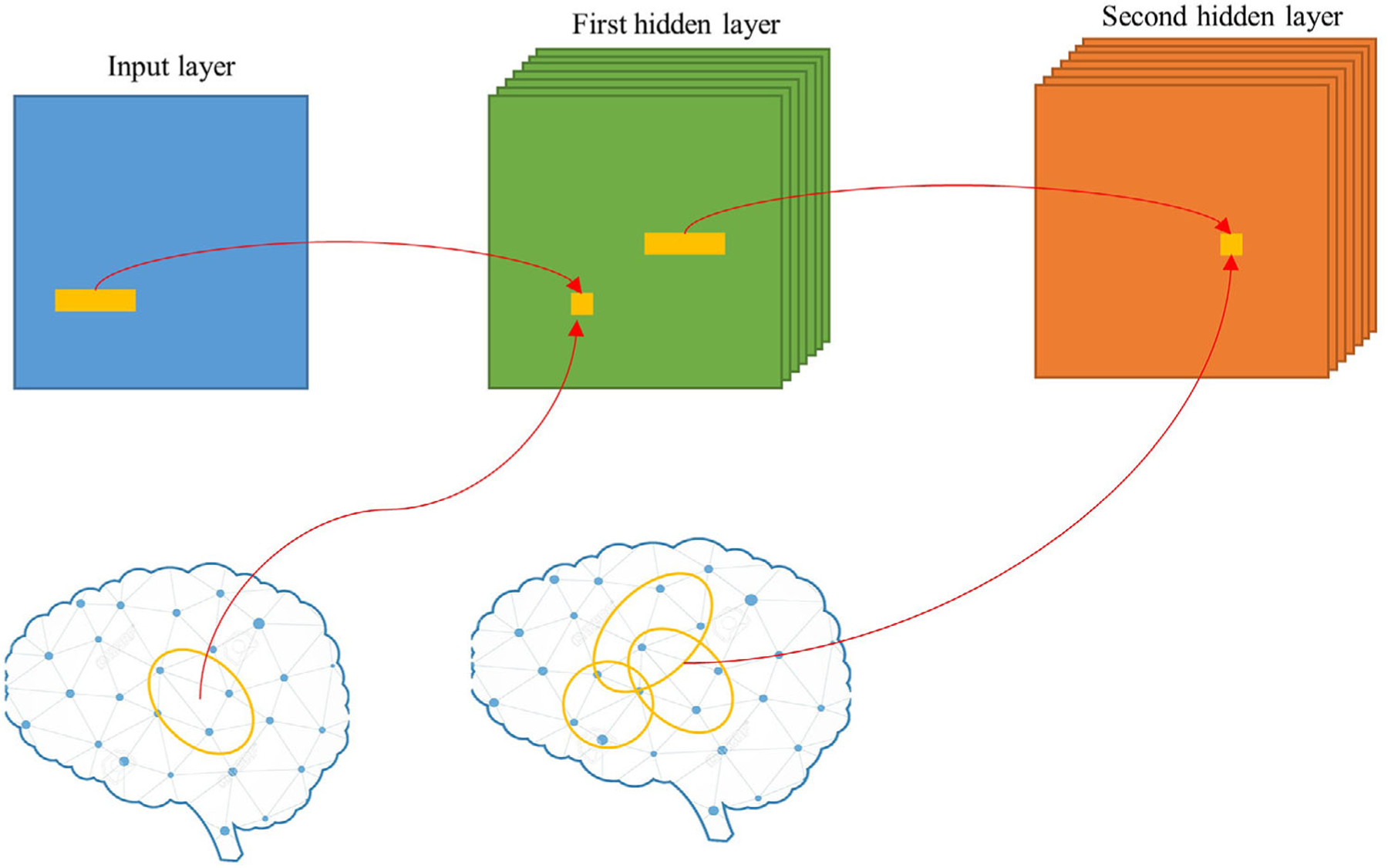
A vector-shaped filter to extract topological information from the brain connectome. For explanatory simplicity, the example displays single-size filter and pooling operation is omitted
The convolution process in layer I is defined as:
| (5) |
| (6) |
where denotes the output from layer I and f (⋅) is the activation function.
In this study, given N training samples [x1, x2 … , xi, … , xN−1, xN] from the target cohort as well as their labels [y1, y2, … , yi, … , yN−1, yN], where xi is the ith input sample (i.e., brain connectome) and yi is the corresponding label, the cross-entropy loss function is defined as:
| (7) |
where p(xi) is the predicted probability of xi, W is the weight matrix, and b denotes the bias of the model. In addition to the dichotomized prediction (i.e., classification), the model is trained to perform continuous cognitive score prediction (i.e., regression). A linear unit is applied at the end of the model and optimized a weighted mean absolute error (AE) cost function as follows:
| (8) |
where is the output of the linear unit of the model, that is, the predicted scores. The model is trained with the goal of minimizing this cost function:
| (9) |
In the backpropagation algorithm, every single value in the convolution process is calculated to measure weight change by .
| (10) |
Since is equal to , expanding the previous equation gives:
| (11) |
Then,
| (12) |
The gradient can be represented by:
| (13) |
The weight deltas in each layer can be computed by:
| (14) |
where Ir is the learning rate that controls the amount of change of the model weights in minimizing the estimated cost in each iteration. The weights are updated by:
| (15) |
The proposed model was optimized using Adam,24 a backpropagation gradient descent algorithm. Adam computes adaptive learning rates for weight updating based on the average of recent magnitudes of the gradients , improving computational efficiency.
2.1 |. Model implementation
The ConCeptCNN (Figure 2) consists of four convolutional channels with different sized vector-shaped convolutional filters, ranging from coarse (1 × 3) and medium (1 × 5) to fine (1 × 7) and global (1 × 90). In each coarse, medium, and fine channel, there are two convolutional layers. After each convolutional layer, an average pooling was applied. The outputs of four convolutional channels were concatenated and flattened, then fed to a single channel with two fully connected layers. We applied batch normalization and dropout regularization for the fully connected layers.25,26 The dropout is a regularization technique that randomly selects a certain ratio of neurons and ignores them during each updating step of training. The “dropped-out” neurons will not contribute to the feedforward process, and the weights of these neurons are not updated in backpropagation. Dropout regularization helps avoid model overfitting. The connectome data are complex and very high in dimension, which can result in an overfitted model. When neurons are randomly dropped out during each iteration of training, each neuron will have a chance to get involved to update weights and contribute to the representation of the features. In this way, the model learns multiple, independent, internal representations and is less sensitive to the training samples. Batch normalization is used to solve the internal covariate scaling problem. This method normalizes the mean and variance of inputs in hidden layers, which avoids either too high or too low activation. Batch normalization also speeds up the training process when handling a large number of parameters. The number of layers is searched in a range from 2 to 10, and the number of neurons in each layer is searched between [22, 23, …, 29]. The initial learning rate is set to 0.01, and epoch is set to 50. These hyperparameters were optimized based on validation data during model training/validation before model testing. An implementation of the ConCeptCNN using TensorFlow is publicly available at GitHub (https://github.com/chen2mg/aicad).
FIGURE 2.

An overview of the proposed Connectome–Inception convolutional neural network (ConCeptCNN) model for early prediction of neurodevelopmental disorders using brain connectome
2.2 |. Alternative convolutional methods comparison
The performance of ConCeptCNN model was compared with several state-of-the-art CNN models including traditional CNN,16 BrainNetCNN,15 ConnectomeCNN,23 and InceptionCNN.18 For a fair comparison, all CNN models were implemented with two convolutional layers and two fully connected layers. The rectified linear unit was used as an activation function. Dropout and batch normalization were applied to the fully connected layers. Specifically, the CNN was implemented with two convolutional layers using a box-shaped filter. Average pooling layers were used after the convolutional layers. The BrainNetCNN model was implemented using cross-shaped filters with two convolutional layers and two fully connected layers. The ConnectomeCNN model was implemented using row-by-row filters followed by column-by-column filters. The InceptionCNN model was implemented using the inception module. InceptionCNN is an advanced CNN model using multiple box-shaped convolutional filters for better feature extraction. It was included to further emphasize the prediction performance of using the vector-shaped filter in the proposed model. In InceptionCNN, two convolutional layers and two inception modules were used. The first two convolutional layers used box-shaped filters and the inception modules used multiple box-shaped filters with size of 1 × 1, 3 × 3, and 5 × 5. For all four models, a SoftMax classifier was used for prediction in the output layer. The detailed implementations are displayed in Table 1, and the hyperparameters are defined based on a grid-search manner with the goal of maximal prediction performance.
TABLE 1.
Detailed description of five convolutional neural network (CNN) architectures
| Relevant parameters (number of filters, kernal size, number of output neurons, dropout) |
||||||||
|---|---|---|---|---|---|---|---|---|
| ConCeptCNN |
||||||||
| Layer | Coarse channel | Medium channel | Fine channel | Global channel | Traditional CNN | BrainNetCNN | Connectome CNN | Inception Net |
| 1 | Conv2D 64@1 × 3, ReLU | Conv2D 64@1 × 5, ReLU | Conv2D 64@1 × 7, ReLU | Conv2D 64@1 × 90, ReLU | Conv2D 64@3 × 3, ReLU | E2E 64@1 × 90, 90 × 1 | Conv2D 64@1 × 90, ReLU | Conv2D 64@3 × 3, ReLU |
| 2 | Average pooling 2D | Average pooling 2D | Average pooling 2D | Average pooling 2D | Average pooling 2D | E2E 128@1 × 90, 90 × 1 | Conv2D 128@90 × 1, ReLU | Max pooling 2D |
| 3 | Conv2D 128@1 × 3, ReLU | Conv2D 128@1 × 5, ReLU | Conv2D 128@1 × 7, ReLU | Flatten | Conv2D 128@3 × 3, ReLU | Flatten | Flatten | Conv2D 128@3 × 3, ReLU |
| 4 | Average pooling 2D | Average pooling 2D | Average pooling 2D | Average pooling 2D | FC, 128 | FC, 128 | Max pooling 2D | |
| 5 | Flatten | Flatten | Flatten | Flatten | Dropout, 0.5, Batch Norm | Dropout, 0.5, Batch Norm | Inception Module | |
| 6 | FC, 256 | FC, 128 | FC, 128 | FC, 128 | Inception Module | |||
| 7 | Dropout, 0.5, Batch Norm | Dropout, 0.5, Batch Norm | Dropout, 0.5, Batch Norm | Dropout, 0.5, Batch Norm | Average pooling | |||
| 8 | FC, 256 | FC, 128 | FC, 1 | FC, 1 | Dropout, 0.5 | |||
| 9 | Dropout, 0.5, Batch Norm | Dropout, 0.5, Batch Norm | FC, 1 | |||||
| 13 | FC,1 | FC, 1 | ||||||
Abbreviations: Batch Norm, batch normalization; ConCeptCNN, Connectome–Inception CNN; Conv2D, two-dimensional convolutional layer; E2E, edge-edge convolutional filter; FC, fully connected layer; ReLU, the rectified linear unit activation function.
2.3 |. Experimental design
2.3.1 |. Early prediction of cognitive deficit using structural connectome data in very preterm infants
The structural connectome dataset included 80 very preterm infants born at or before 31 weeks gestational age. The imaging data were collected between December 2014 and April 2016 from four neonatal intensive care units from the Columbus, OH region, including Nationwide Children’s Hospital (NCH), Ohio State University Medical Center, Riverside Hospital, and Mount Carmel St. Ann’s Hospital. Infants with cyanotic congenital heart disease or other anomalies, such as other congenital birth defects or chromosomal disorders that may possibly affect the central nervous system, were excluded from the study. This study was approved by the Institutional Review Board of NCH, and approval at all other hospitals was obtained through reciprocity agreements with NCH. Written informed consent was obtained from parents or legal guardians of all infants. The DTI data scan parameters can be found in Chen et al.3 The very preterm infants were assessed using standardized Bayley Scales of Infant and Toddler Development-III tests at 2 years corrected age while blinded to DTI data. The Bayley-III cognitive scores were on a scale of 40–160, with a mean of 100 and a standard deviation of 15.
The acquired DTI data were processed, and the brain structural connectivity were constructed using the same pipeline as in Chen et al.3 Briefly, head motion and eddy current artifacts were corrected using FMRIB’s Diffusion Toolbox (FMRIB Software Library, FSL, Oxford, UK). Diffusion tensor reconstruction and brain fiber tracking used Diffusion Toolkit/TrackVis.27 The fiber tracking was performed employing a deterministic tracking algorithm and used an angular threshold of 35° with fiber length threshold of 5 mm.28 The obtained fractional anisotropy maps were harmonized using a batch effect correction algorithm ComBat.29 The weights of structural connectivity between each pair of ROIs were calculated as the mean fractional anisotropy of all voxels along the white matter tract constructed between the two ROIs, resulting in a 90 × 90 symmetric adjacency matrix. This was performed using the UCLA Multimodal Connectivity Package,30 and the connectivity construction was based on a neonatal automated labeling atlas.31
The prediction (i.e., two-class classification) performance of the proposed model was evaluated using a fivefold cross-validation (CV) scheme. Specifically, the datasets were randomly divided into five portions. While four portions were used as training data (70% was further split for model training and 30% for model validation), the remaining portion was used for testing. This process was repeated five times until all portions of the dataset were treated as testing data. Accuracy, sensitivity, specificity, and the area under the receiver operating characteristic curve (AUC) were reported to evaluate the predicting performance. In addition to binary classification, cognitive score prediction (i.e., regression) also was performed. The output layer was replaced with a linear function and the mean-squared error was used as the loss function in the regression. Pearson’s correlation coefficient, mean AE, and standard deviation of absolute error (STD of AE) were calculated and reported. The CV experiment was repeated 50 times to reduce the variability and the averaged results were reported.
The number of preterm infants in the study cohort was relatively small and imbalanced (i.e., only a small portion of the cohort were at high risk for cognitive deficit). The synthetic minority over-sampling technique (SMOTE)32 was utilized to balance and augment the training set. Specifically, the training subjects were divided into five bins according to their Bayley-III cognitive scores (<70, 70–80, 80–90, 90–100, >100). Given a bin, a sample was randomly chosen. Then, k nearest neighbors for the selected sample were searched. We empirically set k = 5 in this work. A synthetic sample xsyn was calculated using the randomly selected sample and its associated neighbors x1, x2, x3, x4, x5, x6 by: xsyn = w1x1 + w2x2 + w3x3 + w4x4 + w5x5 + w6x6, where w1, w2, w3, w4, w5, and w6 are random weights and w1 + w2 + w3 + w4 + w5 + w6 = 1. Similarly, the label ysyn for xsyn was calculated in the same way. The synthetic sample was placed in the given bin. This process was repeated until the number of training subjects reaches 10 times of the original training dataset.
In addition to the prediction study, we want to identify which brain connectivity contributed most to the prediction task. A feature ranking method was implemented to calculate the most discriminative weights in the deep learning model.33 Specifically, the partial derivatives of the output y with regard to the summarized weights of regions Ri were calculated. A higher absolute value of the partial derivative of the connectivity indicates a higher importance for the prediction tasks.
2.3.2 |. ADHD classification using functional connectome data
The functional brain connectome was constructed using resting-state functional MRI (rsfMRI) from the public Neuro Bureau ADHD-200 repository.34 The ADHD-200 dataset consists of 973 anonymized subjects collected from eight different imaging sites: Peking University, Bradley Hospital (Brown University), Kennedy Krieger Institute, The Donders Institute, New York University Child Study Center, Oregon Health and Science University, University of Pittsburgh, and Washington University in St. Louis. The research ethics review boards approved each cohort for every site and signed written informed consent was obtained from participants (or legal guardians) before participation. The large number of subjects collected across different imaging sites and scanned using different parameters offers a unique opportunity for developing a robust learning model. The rsfMRI data were preprocessed using Athena pipeline and a detailed description of data acquisition and preprocessing is publicly available.34 The functional brain connectome was constructed based on a functional defined atlas CC200 in ADHD-200,35 and the connectivity weights were calculated as the Pearson’s correlation coefficient between each pair of ROIs (190 ROIs in total), resulting in a 190 × 190 symmetric adjacency matrix. ADHD subjects were labeled into four categories: (1) healthy controls; (2) ADHD hyperactive; (3) ADHD inattentive; and (4) ADHD combined. In this study, all sub-types of ADHD (i.e., categories 2–4) were combined into one patient group (325 subjects), in contrast with the control group (547 subjects), for binary classification.
In addition to CV, the ADHD-200 consortium officially split the ADHD datasets into a training set (80%) and holdout set (20%). The proposed model was evaluated using holdout set for validation. Specifically, the proposed models were trained using the training cohort and were tested using an independent holdout cohort. Accuracy, sensitivity, specificity, and the AUC were calculated to evaluate the prediction performance. The experiments were repeated 50 times to investigate the variability. Mean and standard deviation results were reported. The discriminative brain connectivity weights associated with ADHD were identified using the same regions feature ranking methods described above.
3 |. RESULTS
All the experiments were performed on a Windows 10 workstation with Intel Xeon Silver 4116 CPU @ 2.10 GHz, 128 GB RAM, and dual Nvidia GTX 1080 Ti GPUs, Santa Clara, CA, USA. The average inference time for an individual sample is around 13 ms.
3.1 |. Early prediction of cognitive deficit using structural connectome data in very preterm infants
The brain structural connectome had a total of 80 very preterm infants with 30 subjects excluded out of 110 subjects due to large motion artifacts and missing labels. The remaining subjects had a mean (SD) gestational age at birth of 28.0 (2.4) weeks and mean postmenstrual age at the time of the MRI scan of 40.4 (0.6) weeks. Forty-one (51.3%) were male. The mean (SD) birth weight of the cohort was 1091.5 g (385.3 g). Infants with Bayley-III cognitive scores less than 90 were labeled as high-risk group (31 subjects) and infants with Bayley-III cognitive scores greater than or equal to 90 were labeled as low-risk group (49 subjects) to develop later moderate/severe cognitive deficits.36
As shown in Table 2, the proposed ConCeptCNN was able to identify high-risk infants for cognitive deficits with a mean (± SD) accuracy of 81.6% (± 4.8%) and an AUC of 0.81 (± 0.03). Compared with other peer convolutional methods, including the traditional CNN,16 BrainNetCNN,15 ConnectomeCNN,23 and InceptionCNN,18 the proposed model achieved a higher AUC by 0.13 (p < 0.001), 0.08 (p < 0.001), 0.06 (p < 0.001), and 0.11 (p < 0.001), respectively.
TABLE 2.
Performance comparison of our proposed Connectome–Inception convolutional neural network (ConCeptCNN) model versus other peer CNN models for the identification of high-risk infants for cognitive deficits using brain structural connectome
| Models | CNN filter | Accuracy (%) | Specificity (%) | Sensitivity (%) | AUC |
|---|---|---|---|---|---|
| Traditional CNN | Box-shaped filter | 71.8 ± 3.3 | 76.3 ± 3.2 | 68.5 ± 6.3 | 0.68 ± 0.05 |
| BrainNetCNN | Cross-shaped filter | 75.2 ± 5.7 | 77.6 ± 3.8 | 71.7 ± 5.1 | 0.73 ± 0.05 |
| ConnectomeCNN | Row-shaped filter | 76.5 ± 4.3 | 80.5 ± 4.7 | 74.6 ± 3.6 | 0.75 ± 0.04 |
| InceptionCNN | Box-shaped filter | 72.4 ± 4.1 | 74.4 ± 5.4 | 66.4 ± 4.2 | 0.70 ± 0.04 |
| ConCeptCNN | Vector-shaped filter | 81.6 ± 4.8 | 83.6 ± 5.6 | 78.3 ± 4.2 | 0.81 ± 0.03 |
Note: data after “±” are standard deviation.
Abbreviations: AUC, area under the receiver operating characteristic curve; Time, average training time (minutes) for one iteration.
In the regression task as shown in Table 3, the Pearson’s correlation coefficients between the predicted and actual Bayley-III cognitive scores were calculated. The proposed ConCeptCNN achieved a correlation coefficient of 0.41 ± 0.05 (p < 0.001). The regression performance outperformed the traditional CNN (0.22 ± 0.07), the BrainNetCNN (0.32 ± 0.06), the ConnectomeCNN (0.38 ± 0.05), and the InceptionCNN (0.25 ± 0.05). The ConCeptCNN achieved the lowest mean STD of AE of 9.3.
TABLE 3.
Performance comparison of our proposed Connectome–Inception convolutional neural network (ConCeptCNN) model versus other peer CNN models for the prediction of cognitive scores in very preterm infants at 2 years of corrected age
| Models | r | p | MAE | STD of AE |
|---|---|---|---|---|
| Traditional CNN | 0.22 ± 0.07 | 0.04 | 25.4 | 13.8 |
| BrainNetCNN | 0.32 ± 0.06 | <0.001 | 18.2 | 11.3 |
| ConnectomeCNN | 0.38 ± 0.05 | <0.001 | 15.6 | 10.4 |
| InceptionCNN | 0.25 ± 0.05 | 0.03 | 23.6 | 12.4 |
| ConCeptCNN | 0.41 ± 0.05 | <0.001 | 14.2 | 9.3 |
Note: p is the p-value of Student t-test of r; r is the Pearson correlation between true and predicted Bayley-III cognitive scores.
Abbreviations: MAE, mean absolute error; STD of AE, standard deviation of absolute error.
3.2 |. ADHD classification using functional connectome data
The functional connectome dataset consisted of 872 subjects after excluding 101 subjects due to missing labels or data quality problems. The subjects had a mean (SD) age at the scan of 12.0 (3.3) years and 567 (65%) were male subjects. There were 325 subjects with ADHD condition and 547 normally developed subjects.
As shown in Table 4, in the CV, our model detected subjects with ADHD with a mean (± SD) accuracy of 78.7% (± 4.3%) and an AUC of 0.75 (± 0.04). Compared with the traditional CNN,16 BrainNetCNN,15 ConnectomeCNN,23 and InceptionCNN,18 the proposed model achieved a higher AUC by 0.1 (p < 0.001), 0.02 (p < 0.05), 0.07 (p < 0.001), and 0.04 (p < 0.001), respectively.
TABLE 4.
Performance comparison of our proposed Connectome–Inception convolutional neural network (ConCeptCNN) model versus other peer CNN models for the detection of attention deficit hyperactivity disorder (ADHD) using brain functional connectome
| Models | CNN filter | Accuracy (%) | Specificity (%) | Sensitivity (%) | AUC |
|---|---|---|---|---|---|
| Traditional CNN | Box-shaped filter | 70.5 ± 5.6 | 73.5 ± 6.8 | 63.3 ± 7.2 | 0.65 ± 0.07 |
| BrainNetCNN | Cross-shaped filter | 76.9 ± 4.7 | 78.3 ± 5.2 | 70.5 ± 6.4 | 0.73 ± 0.05 |
| ConnectomeCNN | Row-shaped filter | 73.1 ± 5.3 | 75.3 ± 4.4 | 65.4 ± 6.2 | 0.68 ± 0.06 |
| InceptionCNN | Box-shaped filter | 75.6 ± 6.3 | 77.4 ± 4.6 | 67.4 ± 5.7 | 0.71 ± 0.06 |
| ConCeptCNN | Vector-shaped filter | 78.7 ± 4.3 | 80.6 ± 4.2 | 73.4 ± 5.7 | 0.75 ± 0.04 |
Note: Data after “±” are standard deviation.
Abbreviations: AUC, area under the receiver operating characteristic curve; Time, average training time (minutes) for one iteration.
The ADHD-200 consortium splits the dataset into a training set and a holdout set for ADHD-200 competition. We used 716 subjects from the training set to train the model and 156 holdout subjects to test. The proposed model achieved an accuracy of 73.6%, with a specificity of 75.6% and a sensitivity of 68.4%. The model also achieved an AUC of 0.71. Table 5 displays the detection comparison results with other research works using the same ADHD holdout datasets.37–40
TABLE 5.
Performance comparison of our proposed Connectome–Inception convolutional neural network (ConCeptCNN) model versus other machine learning methods for the detection of attention deficit hyperactivity disorder (ADHD) using brain functional connectome
| Research works | Methods | Accuracy (%) | Specificity (%) | Sensitivity (%) | AUC |
|---|---|---|---|---|---|
| Dey et al.37 | PCA-LDA | 69.59 | 87.10 | 48.72 | N/A |
| Dai et al.39 | Decision-tree | 61.50 | 77.66 | 41.30 | 0.62 |
| Dey et al.38 | SVM | 73.55 | 72.73 | 75.00 | N/A |
| Sen et al.40 | SVM | 68.92 | 68.32 | 60.00 | N/A |
| ConCeptCNN | Vector-shaped filter | 73.6 ± 4.8 | 75.6 ± 5.4 | 68.4 ± 4.1 | 0.71 ± 0.04 |
Note: Data after “±” are standard deviation.
Abbreviations: AUC, area under the receiver operating characteristic curve; PCA-LDA, principal component analysis–linear discriminant analysis; SVM, support vector machine.
3.3 |. Discriminative brain regions of cognitive deficit in very preterm infants and ADHD in children
Table 6 displays the 15 brain regions that contributed the most toward the learning tasks. For prediction of cognitive deficit using brain structural connectome, 40% of regions were within the right hemisphere and 60% in the left hemisphere. The structural brain regions span frontal, parietal, temporal, and occipital lobes. For the prediction of ADHD using brain functional connectome, 47% of regions were within the right hemisphere and 53% were within the left hemisphere. The functional brain regions span the frontal, temporal, and occipital lobes. The top discriminative regions associated with cognitive deficits and ADHD are displayed using BrainNet Viewer41 in Figures 3 and 4, respectively.
TABLE 6.
Top discriminative clinical features ranked by our Connectome–Inception convolutional neural network (ConCeptCNN) model for the prediction of cognitive deficit (structural connectome) and attention deficit hyperactivity disorder (ADHD) (functional connectome)
| Cognitive deficit (very preterm infants) |
ADHD (children) |
||
|---|---|---|---|
| Brain regions | Weights | Brain regions | Weights |
| Hippocampus right | 1.0 | Superior frontal gyrus (dorsal) left | 1.0 |
| Hippocampus left | 0.9 | Superior frontal gyrus (dorsal) right | 0.8 |
| Insula left | 0.9 | Parahippocampal gyrus left | 0.8 |
| Precuneus left | 0.9 | Superior frontal gyrus (medial) right | 0.8 |
| Precuneus right | 0.9 | Rectus gyrus right | 0.8 |
| Putamen left | 0.8 | Fusiform gyrus left | 0.7 |
| Parahippocampal gyrus right | 0.8 | Middle frontal gyrus right | 0.7 |
| Putamen right | 0.8 | Orbitofrontal cortex (superior) right | 0.7 |
| Middle occipital gyrus left | 0.8 | Rectus gyrus left | 0.7 |
| Lingual gyrus left | 0.8 | Orbitofrontal cortex (middle) left | 0.7 |
| Superior frontal gyrus (dorsal) left | 0.8 | Superior temporal gyrus right | 0.7 |
| Superior frontal gyrus (dorsal) right | 0.7 | Inferior parietal lobule left | 0.6 |
| Parahippocampal gyrus left | 0.7 | Orbitofrontal cortex (middle) right | 0.6 |
| Middle occipital gyrus right | 0.7 | Fusiform gyrus right | 0.6 |
| Orbitofrontal cortex (superior) left | 0.6 | Cuneus left | 0.5 |
FIGURE 3.

Top discriminative brain regions associated with cognitive deficit in very preterm infants identified by the Connectome–Inception convolutional neural network (ConCeptCNN) model
FIGURE 4.

Top discriminative brain regions associated with attention deficit hyperactivity disorder (ADHD) in adolescents identified by the Connectome–Inception convolutional neural network (ConCeptCNN) model
4 |. DISCUSSION
We have demonstrated that the brain topological features can be learned by the proposed ConCeptCNN for prediction of neurodevelopmental disorders. In this proposed model, we used the vector-shaped convolutional filter to capture discriminative features from spatially related ROIs. We designed the CNN model with multiple channels, and in each channel, the topological features are extracted at a different scale. This architecture provides supplementary information for a comprehensive understanding of brain-based disorders within different brain regions as well as across the entire brain. This model is robust to predict different brain disorders using both structural connectome and functional connectome data.
The ConCeptCNN achieved promising performance predicting cognitive outcome (i.e., standardized Bayley-III cognitive scores) in very preterm infants and ADHD outcome in adolescents using brain connectome data. For cognitive deficits prediction, the model achieved an accuracy of 82% and an AUC of 0.81. In the cognitive score regression experiments, our model achieved the best Pearson’s correlation coefficient over multiple peer CNN models. For ADHD outcome prediction, the model achieved an accuracy of 79% and an AUC of 0.75. In addition, the proposed model achieved similar results using holdout datasets in ADHD detection.
Compared with existing peer CNN models, the proposed ConCeptCNN achieved improved performance in early prediction of cognitive deficit in very preterm infants and ADHD outcome prediction in adolescents. In the traditional CNN and InceptionCNN, the brain connectome is treated as 2D images and box-shaped filters are used to extract spatial information from the brain connectome. However, the topological structure in the brain connectome does not match the 2D locality extracted using box-shaped filters. The brain connectome are constructed by an anatomically defined atlas.35 We used a neonatal AAL brain atlas for structural connectome and a CC200 brain atlas for functional connectome. The brain regions in these atlases are permuted based on anatomical structures and most spatially nearby regions are ordered adjacently. In the adjacency matrix of the brain connectome, the brain regions near each other are typically close to each other in rows in the brain atlas. Therefore, the vector-shaped filter can always extract topological features from a cluster of nearby brain regions in the brain connectome. With a series of consecutive layers, a higher level of topological features is integrated for prediction. For the BrainNetCNN and ConnectomeCNN, fixsized global filters are used to extract topological features from the brain connectome. The global convolutional operation aggregates connectivity weights from all brain regions at a time, which can possibly extract features from irrelevant brain regions and generate redundant information, thus, decrease the prediction performance. To address this issue, the ConCeptCNN consisted of four convolutional channels with different sized vector-shaped convolutional filters, ranging from coarse (1 × 3) and medium (1 × 5) to fine (1 × 7) and global (1 × 90). In this way, the model is able to learn detailed topological features from different brain regions. In the backpropagation algorithm, irrelevant features are ignored by updating the neuron weights. We believe such a design provides insight to capture latent information and topological features embedded in the brain connectome for an improved prediction performance.
Brain connectome has demonstrated promising predictive power in many brain disorder studies.3,4,42 The spatial and topological information is discriminative for prediction. In this study, the structural brain connectome was constructed using an infant brain atlas, and the atlas is developed based on an anatomical parcellation of brain regions. Spatially nearby brain regions are ordered adjacently in this atlas. Similarly, the functional connectome was constructed using a functionally defined atlas,31,35 and spatially coherent brain regions are clustered together in developing the atlas. In this way, as the convolutional filters move across rows and columns of the brain connectome matrix, the ConCeptCNN model was able to capture anatomical and topological information for prediction. We tested the proposed model using a randomly permuted brain connectome matrix. Specifically, we ordered the ROIs randomly and constructed the brain connectome based on the random order. We tested the model with the randomly permutated brain connectome using the same fivefold CV and repeated the experiments 50 times. The model achieved an accuracy of 65.3% and an AUC of 0.66 on cognitive score prediction, and an accuracy of 63.4%, and an AUC of 0.62 on ADHD detection. These results were significantly lower than the performance using an anatomically constructed connectome.
In our study, the structural connectome datasets were obtained from a very preterm infant cohort and the functional connectome datasets were acquired from the ADHD-200 consortium. Both datasets are imbalanced with a smaller number of condition subjects versus a larger number of control subjects. With such imbalanced datasets, the deep learning model is likely to predict condition subjects (in minority group) as control subjects (in majority group), thus resulting in high specificity and low sensitivity performance. To mitigate the impact of data imbalance, we applied data balancing and augmentation techniques before training the model.
The identification of discriminative brain regions is significant in understanding the etiology behind brain disorders. The ConCeptCNN ranked the brain regions based on their contribution toward the learning tasks on cognitive deficit prediction and ADHD detection.3,7 In the cognitive deficit study, the identified brain regions such as the hippocampus (learning, memory), putamen, superior frontal gyrus (cognitive functions, memory), middle occipital gyrus, and orbitofrontal cortex have been reported in previous independent studies,43,44 and have been proved to be associated with brain cognitive functions. For example, Anand and Dhikav discussed that the hippocampus is a complex brain structure that plays an important role in learning and memory. du Boisgueheneuc et al. believed that the superior frontal gyrus is an important brain region associated with cognitive functions and particularly contributed to the working memory system. For the ADHD study, several top-ranked regions including the superior frontal gyrus, middle frontal gyrus (literacy), rectus gyrus, orbitofrontal cortex (emotion), fusiform gyrus (object recognition), and cuneus also have been reported in other studies.45–47 The middle frontal gyrus regions are thought to be associated with the development of literacy such as reading and numeracy,45 which have a significant impact on academic studies in adolescence. Furthermore, orbitofrontal cortex regions have an association with emotional control and emotion-guided behaviors.46 The identified fusiform gyrus regions are related to high-level vision functions such as face perception, object recognition, and reading.47
There are limitations to our study. First, we designed the ConCeptCNN model with multiple channels using different sizes of convolutional filters and several layers. Such an architecture is achieved by “brute force” searching to achieve the best prediction performance. However, the searching space is limited by the computational power of existing computer hardware. Second, although we tested the model using datasets with two types of neurodevelopmental disorders and the number of subjects is considered large in this field, we need to further validate the model using even larger datasets from a variety of additional brain disorders to assess its clinical utility.
5 |. CONCLUSION
In summary, we propose ConCeptCNN to predict neurodevelopmental disorders using brain connectome data. In this model, we use vector-shaped filters to better capture the brain connectome topological information from spatially related ROIs. In addition, instead of a single-size filter, we propose to use multi-size filters that can provide supplementary information for comprehensive understanding within different brain regions and across the entire brain. We tested the proposed model using structural and functional connectome datasets. The performance of the proposed ConCeptCNN was compared with several peer CNN models including the traditional CNN,16 InceptionCNN,18 BrainNetCNN,15 and ConnectomeCNN.23 Both brain structural and brain functional connectome were used for evaluation and comparison. In the CV experiments, the proposed model outperformed other CNN methods in early prediction of cognitive deficit in very preterm infants and ADHD detection in adolescents.
ACKNOWLEDGMENTS
The authors declare that the research was conducted in the absence of any commercial or financial relationships that could be construed as a potential conflict of interest. This work was supported by the National Institutes of Health (R01-EB029944, R01-EB030582, R21-HD094085, R01-NS094200 and R01-NS096037), and a Trustee grant from Cincinnati Children’s Hospital Medical Center. The funders played no role in the design, analysis, or presentation of the findings.
Funding information
National Institutes of Health, Grant/Award Numbers: R01-EB029944, R01-EB030582, R21-HD094085, R01-NS094200, R01-NS096037; Trustee grant from Cincinnati Children’s Hospital Medical Center
Footnotes
CONFLICT OF INTEREST
The authors have no conflicts to disclose.
REFERENCES
- 1.Sporns O The human connectome: origins and challenges. Neuroimage 2013;80:53–61. [DOI] [PubMed] [Google Scholar]
- 2.Glasser MF, Smith SM, Marcus DS, et al. The Human Connectome Project’s neuroimaging approach. Nat Neurosci 2016;19(9):1175–1187. [DOI] [PMC free article] [PubMed] [Google Scholar]
- 3.Chen M, Li HL, Wang JH, et al. Early prediction of cognitive deficit in very preterm infants using brain structural connectome with transfer learning enhanced deep convolutional neural networks. Front Neurosci 2020;14:858. [DOI] [PMC free article] [PubMed] [Google Scholar]
- 4.He L, Li H, Holland SK, Yuan W, Altaye M, Parikh NA. Early prediction of cognitive deficits in very preterm infants using functional connectome data in an artificial neural network framework. NeuroImage Clinical 2018;18:290–297. [DOI] [PMC free article] [PubMed] [Google Scholar]
- 5.Li HL, Parikh NA, He LL. A novel transfer learning approach to enhance deep neural network classification of brain functional connectomes. Front Neurosci 2018;12:491. [DOI] [PMC free article] [PubMed] [Google Scholar]
- 6.Dennis EL, Thompson PM. Functional brain connectivity using fMRI in aging and Alzheimer’s disease. Neuropsychol Rev 2014;24(1):49–62. [DOI] [PMC free article] [PubMed] [Google Scholar]
- 7.Chen M, Li H, Wang J, Dillman JR, Parikh NA, He L. A multichannel deep neural network model analyzing multiscale functional brain connectome data for attention deficit hyperactivity disorder detection. Radiol Artif Intell 2019;2(1):e190012. [DOI] [PMC free article] [PubMed] [Google Scholar]
- 8.Riaz A, Asad M, Alonso E, Slabaugh G. Fusion of fMRI and non-imaging data for ADHD classification. Comput Med Imaging Graph 2018;65:115–128. [DOI] [PubMed] [Google Scholar]
- 9.Watanabe T, Kessler D, Scott C, Angstadt M, Sripada C. Disease prediction based on functional connectomes using a scalable and spatially-informed support vector machine. Neuroimage 2014;96:183–202. [DOI] [PMC free article] [PubMed] [Google Scholar]
- 10.Zhang X, Hu B, Ma X, Xu L. Resting-state whole-brain functional connectivity networks for MCI classification using L2-regularized logistic regression. IEEE Trans Nanobiosci 2015;14(2):237–247. [DOI] [PubMed] [Google Scholar]
- 11.Kim J, Calhoun VD, Shim E, Lee JH. Deep neural network with weight sparsity control and pre-training extracts hierarchical features and enhances classification performance: evidence from whole-brain resting-state functional connectivity patterns of schizophrenia. Neuroimage 2016;124(pt A):127–146. [DOI] [PMC free article] [PubMed] [Google Scholar]
- 12.Heinsfeld AS, Franco AR, Craddock RC, Buchweitz A, Meneguzzi F. Identification of autism spectrum disorder using deep learning and the ABIDE dataset. NeuroImage Clin 2017;17:16–23. [DOI] [PMC free article] [PubMed] [Google Scholar]
- 13.Guo X, Dominick KC, Minai AA, Li H, Erickson CA, Lu LJ. Diagnosing autism spectrum disorder from brain resting-state functional connectivity patterns using a deep neural network with a novel feature selection method. Front Neurosci 2017;11:460. [DOI] [PMC free article] [PubMed] [Google Scholar]
- 14.Munsell BC, Wee CY, Keller SS, et al. Evaluation of machine learning algorithms for treatment outcome prediction in patients with epilepsy based on structural connectome data. Neuroimage 2015;118:219–230. [DOI] [PMC free article] [PubMed] [Google Scholar]
- 15.Kawahara J, Brown CJ, Miller SP, et al. BrainNetCNN: convolutional neural networks for brain networks; towards predicting neurodevelopment. Neuroimage 2017;146:1038–1049. [DOI] [PubMed] [Google Scholar]
- 16.LeCun Y, Bengio Y, Hinton G. Deep learning. Nature 2015;521(7553):436–444. [DOI] [PubMed] [Google Scholar]
- 17.Simonyan K, Very deep convolutional networks for large-scale image recognition. arXiv preprint arXiv:1409.1556 (2014). [Google Scholar]
- 18.Szegedy C, Liu W, Jia YQ, et al. Going deeper with convolutions. In: 2015 IEEE Conference on Computer Vision and Pattern Recognition (CVPR). IEEE; 2015:1–9. [Google Scholar]
- 19.He K, Zhang X, Ren S, Sun J. Deep residual learning for image recognition. Paper presented at: Proceedings of the IEEE Conference on Computer Vision and Pattern Recognition. 2016. [Google Scholar]
- 20.Qureshi MNI, Oh J, Lee B. 3D-CNN based discrimination of schizophrenia using resting-state fMRI. Artif Intell Med 2019;98:10–17. [DOI] [PubMed] [Google Scholar]
- 21.Du Y, Li B, Hou Y, Calhoun VD. A deep learning fusion model for brain disorder classification: application to distinguishing schizophrenia and autism spectrum disorder. ACM BCB 2020;2020:56. [DOI] [PMC free article] [PubMed] [Google Scholar]
- 22.Fan L, Su J, Qin J, Hu D, Shen H. A deep network model on dynamic functional connectivity with applications to gender classification and intelligence prediction. Front Neurosci 2020;14:881. [DOI] [PMC free article] [PubMed] [Google Scholar]
- 23.Meszlényi RJ, Buza K, Vidnyánszky Z. Resting state fMRI functional connectivity-based classification using a convolutional neural network architecture. Front Neuroinform 2017;11:61. [DOI] [PMC free article] [PubMed] [Google Scholar]
- 24.Kingma DP, Ba J. Adam: a method for stochastic optimization. In: The 3rd International Conference for Learning Representations, San Diego. 2015. [Google Scholar]
- 25.Ioffe S, Szegedy C. Batch normalization: accelerating deep network training by reducing internal covariate shift. Paper presented at: International Conference on Machine Learning. 2015. [Google Scholar]
- 26.Srivastava N, Hinton G, Krizhevsky A, Sutskever I, Salakhutdinov R. Dropout: a simple way to prevent neural networks from overfitting. J Mach Learn Res 2014;15(1):1929–1958. [Google Scholar]
- 27.Hess CP, Mukherjee P, Han ET, Xu D, Vigneron DB. Q-ball reconstruction of multimodal fiber orientations using the spherical harmonic basis. Magn Reson Med 2006;56(1):104–117. [DOI] [PubMed] [Google Scholar]
- 28.Wang R, Benner T, Sorensen AG, Wedeen VJ. Diffusion toolkit: a software package for diffusion imaging data processing and tractography. Paper presented at: Proceedings of the International Society of Magnetic Resonance in Medicine. 2007. [Google Scholar]
- 29.Fortin JP, Parker D, Tunc B, et al. Harmonization of multi-site diffusion tensor imaging data. Neuroimage 2017;161:149–170. [DOI] [PMC free article] [PubMed] [Google Scholar]
- 30.Bassett DS, Brown JA, Deshpande V, Carlson JM, Grafton ST. Conserved and variable architecture of human white matter connectivity. Neuroimage 2011;54(2):1262–1279. [DOI] [PubMed] [Google Scholar]
- 31.Shi F, Yap PT, Wu GR, et al. Infant brain atlases from neonates to 1- and 2-year-olds. PLoS One 2011;6(4):e18746. [DOI] [PMC free article] [PubMed] [Google Scholar]
- 32.Chawla NV, Bowyer KW, Hall LO, Kegelmeyer WP. SMOTE: synthetic minority over-sampling technique. J Artif Intell Res 2002;16:321–357. [Google Scholar]
- 33.Simonyan K, Vedaldi A, Zisserman A. Deep Inside Convolutional Networks: Visualising Image Classification Models and Saliency Maps 2013. [Google Scholar]
- 34.Bellec P, Chu C, Chouinard-Decorte F, Benhajali Y, Margulies DS, Craddock RC. The Neuro Bureau ADHD-200 preprocessed repository. Neuroimage 2017;144(pt B):275–286. [DOI] [PubMed] [Google Scholar]
- 35.Craddock RC, James GA, Holtzheimer PE 3rd, Hu XP, Mayberg HS. A whole brain fMRI atlas generated via spatially constrained spectral clustering. Hum Brain Mapp 2012;33(8):1914–1928. [DOI] [PMC free article] [PubMed] [Google Scholar]
- 36.Spencer-Smith MM, Spittle AJ, Lee KJ, Doyle LW, Anderson PJ. Bayley-III cognitive and language scales in preterm children. Pediatrics 2015;135(5):e1258–e1265. [DOI] [PubMed] [Google Scholar]
- 37.Dey S, Rao AR, Shah M. Exploiting the brain’s network structure in identifying ADHD subjects. Frontiers in Systems Neuroscience 2012;6:75. [DOI] [PMC free article] [PubMed] [Google Scholar]
- 38.Dey S, Rao AR, Shah M. Attributed graph distance measure for automatic detection of attention deficit hyperactive disordered subjects. Front Neural Circuits 2014;8:64. [DOI] [PMC free article] [PubMed] [Google Scholar]
- 39.Dai D, Wang J, Hua J, He H. Classification of ADHD children through multimodal magnetic resonance imaging. Front Syst Neurosci 2012;6:63. [DOI] [PMC free article] [PubMed] [Google Scholar]
- 40.Sen B, Borle NC, Greiner R, Brown MRG. A general prediction model for the detection of ADHD and Autism using structural and functional MRI. PLoS One 2018;13(4):e0194856. [DOI] [PMC free article] [PubMed] [Google Scholar]
- 41.Xia MR, Wang JH, He Y. BrainNet viewer: a network visualization tool for human brain connectomics. PLoS One 2013;8(7):e68910. [DOI] [PMC free article] [PubMed] [Google Scholar]
- 42.He T, Kong R, Holmes AJ, et al. Deep neural networks and kernel regression achieve comparable accuracies for functional connectivity prediction of behavior and demographics. Neuroimage 2020;206:116276. [DOI] [PMC free article] [PubMed] [Google Scholar]
- 43.Anand KS, Dhikav V. Hippocampus in health and disease: an overview. Ann Indian Acad Neurol 2012;15(4):239–246. [DOI] [PMC free article] [PubMed] [Google Scholar]
- 44.du Boisgueheneuc F, Levy R, Volle E, et al. Functions of the left superior frontal gyrus in humans: a lesion study. Brain 2006;129(pt 12):3315–3328. [DOI] [PubMed] [Google Scholar]
- 45.Koyama MS, O’Connor D, Shehzad Z, Milham MP. Differential contributions of the middle frontal gyrus functional connectivity to literacy and numeracy. Sci Rep 2017;7(1):17548. [DOI] [PMC free article] [PubMed] [Google Scholar]
- 46.Rolls ET. The orbitofrontal cortex and emotion in health and disease, including depression. Neuropsychologia 2019;128: 14–43. [DOI] [PubMed] [Google Scholar]
- 47.Weiner KS, Zilles K. The anatomical and functional specialization of the fusiform gyrus. Neuropsychologia 2016;83:48–62. [DOI] [PMC free article] [PubMed] [Google Scholar]