Improving trial generalizability using observational studies

Abstract

Complementary features of randomized controlled trials (RCTs) and observational studies (OSs) can be used jointly to estimate the average treatment effect of a target population. We propose a calibration weighting estimator that enforces the covariate balance between the RCT and OS, therefore improving the trial-based estimator’s generalizability. Exploiting semiparametric efficiency theory, we propose a doubly robust augmented calibration weighting estimator that achieves the efficiency bound derived under the identification assumptions. A nonparametric sieve method is provided as an alternative to the parametric approach, which enables the robust approximation of the nuisance functions and data-adaptive selection of outcome predictors for calibration. We establish asymptotic results and confirm the finite sample performances of the proposed estimators by simulation experiments and an application on the estimation of the treatment effect of adjuvant chemotherapy for early-stage non-small-cell lung patients after surgery.

1 |. INTRODUCTION

Randomized controlled trials (RCTs) are the gold standard to evaluate treatment effects. However, due to restrictive inclusion and exclusion criteria, the trial sample is narrowly defined and can be systematically different from the real-world patient population to which the new treatment is supposed to be given. Therefore, the findings from RCTs often lack external validity (Rothwell, 2005). On the other hand, observational studies (OSs) often include large samples that are representative of real-world patient populations; however, there are concerns about whether or not confounding has been addressed adequately in the analyses of OSs. In cancer research, there is an in-depth discussion on the strengths and limitations of utilizing data from RCT and OSs for comparative effectiveness analyses (Korn and Freidlin, 2012).

The problems of extending findings from RCT to a target population has been termed as generalizability (e.g., Cole and Stuart, 2010; Tipton, 2013; Dahabreh et al., 2019) and transportability (e.g., Pearl and Bareinboim, 2011; Rudolph and van der Laan, 2017; Westreich et al., 2017). Most existing methods rely on direct modeling of the sampling score, the sampling analog of the propensity score. The subsequent sampling score adjustments include inverse probability of sampling weighting (IPSW; Cole and Stuart, 2010; Buchanan et al., 2018), stratification (Tipton, 2013), and augmented IPSW (AIPSW; Dahabreh et al., 2019). Most sampling score adjustment approaches require the sampling score model to be correctly specified. Moreover, weighting estimators are unstable if the sampling score is too extreme.

We consider combining an RCT sample and an OS sample to estimate the average treatment effect (ATE) of a target population, where the RCT sample is subject to selection bias and the OS sample is representative of the target population with a known sampling mechanism. In contrast to the dominant approaches that focus on predicting sample selection probabilities, we estimate the sampling score weights directly by calibrating covariates balance between the RCT sample and the design-weighted OS sample to address the selection bias of the RCT sample. Calibration weighting (CW) is widely used to integrate auxiliary information in survey sampling (Wu and Sitter, 2001) and causal inference (Qin and Zhang, 2007; Hainmueller, 2012). Hartman et al. (2015) implemented CW to estimate the population ATEs by combining RCTs with OSs.

The efficiency of the CW estimator can be further improved. We derive the semiparametric efficiency bound for the ATE under the identification assumptions, which provides the benchmark for estimation efficiency. We propose the augmented CW (ACW) estimator that is doubly robust and also achieves the semiparametric efficiency bound when both nuisance models are correctly specified. However, the parametric approach is prone to model misspecification, especially when there is complex confounding. To cope with model misspecification, we adopt a method of sieves (Chen, 2007), which allows flexible data-adaptive estimation of the nuisance functions while the ACW estimator retains the usual root-n consistency under regularity conditions. In comparison with other nonparametric and machine learning methods, the proposed ACW estimator with the sieve approximation is attractive: (1) unlike black-box machine learning methods, calibration weighting is straightforward and transparent; and (2) our framework allows for selecting important sieve basis terms that are related to the outcome to calibrate and enforcing the balance on these covariates for efficient estimation.

In the presence of many covariates, variable or sieve basis selection for calibration becomes necessary. We classify covariates into three types: the covariates that are associated with both trial participation and outcome as confounders, that affect outcome only through trial participation as instrumental variables (IVs), and that are predictive of the outcome as precision variables or outcome predictors. In other causal inference contexts, studies have shown that in addition to the confounding variables, including outcome predictors in the propensity score may improve efficiency, whereas including IVs may decrease efficiency (e.g., Tang et al., 2020). Despite the importance of proper basis selection for the efficient causal estimator, the current literature lacks a principled approach to guide basis selection for covariate balancing. Capitalizing on an explicit connection between calibration weighting and estimating equations under parametric models, we propose a penalized estimating equation approach for variable selection with an emphasis on outcome predictors.

2 |. BASIC SETUP

2.1 |. Notation: Causal effect and two data sources

Let X be the p-dimensional vector of covariates, A be the binary treatment {0, 1}, and Y be the outcome of interest. We use the potential outcomes framework to formulate the causal problem. We assume that each subject has a potential outcome Y(a), a ∈ {0, 1}, representing the outcome had the subject been given the treatment a. The conditional average treatment effect (CATE) is τ(X) = E{Y(1) − Y(0) | X}. We are interested in estimating the population ATE τ₀ = E{τ(X)}, where the expectation is taken with respect to the distribution of the target population. Let δ = 1 denote RCT participation, and let $\tilde{\delta }=1$ denote the OS participation. Also, define the sampling score as π_δ(X) = P(δ = 1 | X), the design weight for the OS sample as $d=1/P(\tilde{\delta }=1\mid X)$, and the conditional outcome mean function as μ_a,δ(X) = E(Y | X, A = a, δ) for a, δ ∈ {0, 1}.

To generalize findings to the future patient population, we consider a superpopulation framework that describes the distribution of all patients with a certain disease to whom the new treatment is intended to be given. The data structure is demonstrated in Figure 1. The RCT is a sample from the target population with an unknown sampling mechanism, and the OS sample is a random sample from the target population with a known sampling mechanism. Therefore, our problem is in line with that of generalizability, extending the ATE result from the trial to its larger population (Dahabreh et al., 2019). A closely related problem is transportability which tries to extend the trial results to an external population (Westreich et al., 2019); for example, when one wants to transport an RCT conducted in one country to a population in another country (Pearl, 2015). Subtle differences exist in the two problems in terms of estimands and identification assumptions; see Web Appendix A for details. In general, there are nested and nonnested study designs in the problem of generalization (Dahabreh et al., 2019). For nested designs, the RCT sample is a sub-sample from the OS sample. Examples include pragmatic trial studies embedded in health care systems or comprehensive cohort studies, where all trial-eligible participants constitute the OS sample, and participants who agree to be randomized constitute the RCT sample. For nonnested designs, the RCT sample and the OS sample are separate. Our motivating application falls in the latter category, where we link an existing RCT to a large cancer register database. We also assume that the RCT and OSs are independent. This assumption holds naturally if the two separate studies are conducted independently by different researchers; it is also plausible in our motivating example where the patients for the two studies were accrued in two separate time periods (see Section 6).

FIGURE 1.

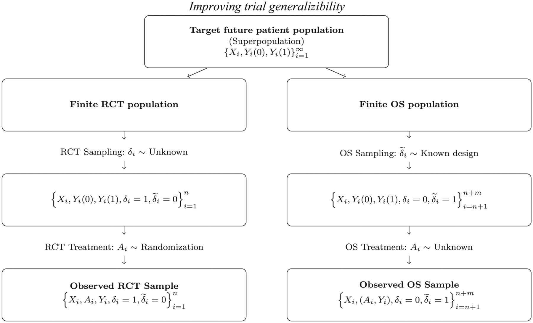
Demonstration of the sampling and treatment assignment regimes for the RCT and OS samples within the target population.

2.2 |. Identification assumptions

To identify the ATE, we make the following assumptions:

Assumption 1 (Consistency). Y = AY(1) + (1 − A)Y(0).

Assumption 2 (Ignorability and positivity of treatment assignment). (i) {Y(0), Y(1)} ⫫ A | (X, δ = 1); and (ii) 0 < P(A = 1 | X, δ = 1) < 1 with probability 1.

Assumption 3 (Generalizability of the CATE and positivity of trial participation). (i) E{Y(1) − Y(0) | X, δ = 1} = τ(X); and (ii) π_δ(X) > 0 with probability 1.

Assumption 1 implies that trial encouragement effects are absent (Dahabreh and Hernán, 2019). Assumption 2 holds for the RCT by default. Assumption 3 (i) is similar to the generalizability in effect measure condition (Dahabreh et al., 2019, Supporting Information). Even though this assumption is formally weaker than the mean exchange-ability over trial participation (Dahabreh et al., 2019), that is, E{Y(a) | X, δ = 1} = E{Y(a) | X} for a = 0, 1, and the ignorability assumption on trial participation (Stuart et al., 2011), that is, {Y(0), Y(1)} ⫫ δ | X, it suffices to identify the ATE. Under Assumptions 1–3, the ATE is identified by ${\tau }_0=E\left[\tilde{\delta }d\left\{{\mu }_{1,1}(X)-{\mu }_{0,1}(X)\right\}\right]$.

Although being essential, Assumption 3 (i) is not verifiable based on the observed data but relies on subject matter experts to assess its plausibility. It is plausible if X captures all variables that are related to the trial participation and outcome (Buchanan et al., 2018). Assumption 3 (ii) requires the absence of patient characteristics that prohibit participation. When Assumption 3 (ii) is violated, generalization can only be made to a restricted population without extrapolation (Yang and Ding, 2018).

2.3 |. Existing estimation methods

Because the RCT assigns treatments randomly to the participants, τ(X) is identifiable and can be estimated by standard estimators solely from the RCT. However, f(X | δ = 1) is different from f(X) in general; therefore, E{τ(X) | δ = 1} is different from τ₀, and the ATE estimator using trial data only is biased of τ₀ generally. A widely used approach is the IPSW estimator that predicts the sampling score π_δ(X) and uses the inverse of the estimated sampling score to account for the shift of the covariate distribution from the RCT sample to the target population. Specifically, most of the empirical literature assumes that π_δ(X) follows a logistic regression model π_δ(X; η) and can be estimated by ${\pi }_{\delta }(X;\widehat{\eta })$. The AIPSW estimator has also been proposed to improve it by employing both the sampling score and outcome regression. The forms of the (A)IPSW estimators are provided in Web Appendix B, along with another identification formula based on the IPSW estimator.

3 |. CALIBRATION WEIGHTING ESTIMATOR

We propose to use calibration originated in survey sampling to eliminate the selection bias in the trial-based ATE estimator. The calibration weighting approach is similar to the idea of entropy balancing weights introduced by Hainmueller (2012). We calibrate subjects in the RCT sample so that after calibration, the covariate distribution of the RCT sample empirically matches the target population. Our insight is that for any vector-valued function g(X), the following equations hold:

$$E\left[\frac{{\left\{{\pi }_{\delta }(X)\right\}}^{-1}\delta }{E\left[{\left\{{\pi }_{\delta }(X)\right\}}^{-1}\delta \right]}g(X)\right]=E\left\{\tilde{\delta }dg(X)\right\}=E\left\{g(X)\right\}.$$ (1)

Here, g(X) contains the covariate functions to be calibrated, which could be moment functions of the original covariate X or any sensible transformations of X. To this end, we assign a weight q_i to each subject i in the RCT sample so that

$$\sum _{i=1}^N{\delta }_i{q}_{i}g\left(X_i\right)=\tilde{g},$$ (2)

where $\tilde{g}={\sum }_{i=1}^N{\tilde{\delta }}_i{d}_{i}g\left(X_i\right)/{\sum }_{i=1}^N{\tilde{\delta }}_i{d}_i$ is a design-weighted estimate of E{g(X)} from the OS sample, and N is the target population size, not necessarily known. Constraint (2) is referred to as the balancing constraint, and weights $\mathcal{Q}=\left\{q_i:{\delta }_i=1\right\}$ are the calibration weights. The balancing constraint calibrates the RCT covariate distribution to the target population in terms of g(X). The choice of g(X) is critical for both bias and variance considerations, which we discuss in Section 4.2.

We estimate $\mathcal{Q}$ by solving the optimization problem:

$$\underset{\mathcal{Q}}{\text{min}}\sum _{i=1}^n{q}_i\text{ log }{q}_i,$$ (3)

subject to q_i ≥ 0 ∀i; ${\sum }_{i=1}^n{q}_i=1$, and the constraint (2), where n is the RCT sample size. The objective function in (3) is the negative entropy of the calibration weights; thus, minimizing these criteria ensures that the empirical distribution of calibration weights is not too far away from the uniform, such that it minimizes the variability due to heterogeneous weights (Owen, 2001). The optimization problem can be solved using convex optimization with the Lagrange multiplier. By introducing the Lagrange multiplier λ, the objective function becomes

$$L(\lambda ,\mathcal{Q})=\sum _{i=1}^n{q}_i\text{ log }{q}_i-{\lambda }^{\top }\left\{\sum _{i=1}^n{q}_{i}g\left(X_i\right)-\tilde{g}\right\}.$$ (4)

Minimizing (4) leads to $\widehat{q_i}=q\left(X_i;\widehat{\lambda }\right)=\text{exp}\left\{{\widehat{\lambda }}^{\top }g\left(X_i\right)\right\}/{\sum }_{i=1}^n\text{exp}\left\{{\widehat{\lambda }}^{\top }g\left(X_i\right)\right\}$ and $\widehat{\lambda }$ solves

$$U(\lambda )=\sum _{i=1}^n\text{exp}\left\{{\mathit{\lambda }}^{\top }g\left(X_i\right)\right\}\left\{g\left(X_i\right)-\tilde{g}\right\}=0,$$ (5)

which is the dual problem to the optimization problem (3).

Let π_Ai = P(A_i = 1|X_i, δ_i = 1) be the treatment propensity score for subject i. For RCTs, it is common that the propensity score π_Ai is known. The CW estimator becomes

$${\widehat{\tau }}^{\text{CW}}=\sum _{i=1}^n{\widehat{q}}_i\left\{\frac{A_i{Y}_i}{{\pi }_{Ai}}-\frac{\left(1-A_i\right)Y_i}{1-{\pi }_{Ai}}\right\}.$$ (6)

To investigate the properties of the CW estimator, we impose the regularity conditions on the sampling designs for the RCT the OS samples.

Assumption 4. Let μ_g0 = E{g(X)}. The design weighted estimator ${\widehat{\mu }}_g=N^{-1}{\sum }_{i=1}^N{\tilde{\delta }}_i{d}_{i}g\left(X_i\right)$ satisfies $V\left({\widehat{\mu }}_g\right)=O\left(m^{-1}\right)$, and ${\left\{V\left({\widehat{\mu }}_g\right)\right\}}^{-1/2}\left({\widehat{\mu }}_g-{\mu }_{g_0}\right)\to \mathcal{N}(0,1)$ in distribution, as m → ∞, where m is the OS sample size.

Assumption 5 (Linearity of the CATE). $\tau (X)={\gamma }_0^{\top }g(X)$.

Assumption 6 (Loglinear sampling score). The sampling score of RCT participation follows a loglinear model, that is, ${\pi }_{\delta }(X)=\text{exp}\left\{{\eta }_0^{\top }g(X)\right\}$ for some η₀.

Based on the above assumptions, we establish the double robustness property of the CW estimator in the following theorem and relegate all proofs to Web Appendix C. The proof is similar to the one in Zhao and Percival (2017).

Theorem 1 (Double robustness of the CW estimators). Under Assumptions 1–4, if either Assumption 5 or 6 holds, ${\widehat{\tau }}^{\text{CW}}$ in (6) is consistent for τ₀.

In the estimation of calibration weights, we only require specifying g(X). Thus, calibration weighting evades explicitly modeling either the sampling score model or the outcome mean models. Under Assumption 6, we show that there is a direct correspondence between calibration weight $q\left(X_i;\widehat{\lambda }\right)$ and the estimated sampling score ${\pi }_{\delta }\left(X_i;\widehat{\eta }\right)$, that is, $q\left(X_i;\widehat{\lambda }\right)={\left\{N{\pi }_{\delta }\left(X_i;\widehat{\eta }\right)\right\}}^{-1}+o_p\left(N^{-1}\right)$. That is, calibration weights from the objective function (3) have the same functional form as inverse probability of sampling score weights under Assumption 6 asymptotically. Other objective functions, such as ${\sum }_{i=1}^n\left(q_i-1\right)\text{log}\left(q_i-1\right)$, ${\sum }_{i=1}^n\left\{q_i\text{ log }{q}_i+\left(1-q_i\right)\text{ log}\left(1-q_i\right)\right\}$ (Zhao, 2019; Josey et al., 2020) or ${\sum }_{i=1}^n{\left(q_i-n^{-1}\right)}^2$ (Chattopadhyay et al., 2020), can also be used. When the sampling score follows a logistic regression model, the objective function ${\sum }_{i=1}^n\left(q_i-1\right)\text{log}\left(q_i-1\right)$ results in weights that resemble the inverse of logistic sampling scores (Zhao, 2019; Josey et al., 2020). However, if the fraction n/N of the RCT sample in the target population is small, the loglinear model in Assumption 6 is close to the logistic regression model; our simulation studies show that the proposed CW estimator is not sensitive to the choice of the objective function for the optimization.

The entropy balancing has been studied in the indirect comparison literature (Signorovitch et al., 2010; Phillippo et al., 2018; Petto et al., 2019). The goal is to adjust for the imbalance between two separate randomized trials with common comparative arms, similar to the transportability problem. On the other hand, the proposed CW estimator is motivated by generalizing findings from RCT. Importantly, building on the CW estimator, we propose an improved estimator capitalizing semiparametric efficiency theory in the next section and a data-adaptive selection of outcome predictors for calibration, which is absent in the literature. The proposed framework can incorporate nonparametric sieve approximation of the outcome mean function and sampling score while providing valid inferences.

4 |. SEMIPARAMETRIC EFFICIENT ESTIMATOR

4.1 |. Augmented calibration weighting estimator

The following theorem gives the semiparametric efficiency bound for τ₀ in our data integration setting. Let Δ_a = Y − μ_a,1(X; β_a).

Theorem 2 (Semiparametric efficiency bound). Under Assumptions 1–4, the semiparametric efficiency score for τ₀ is

$$\varphi (X,A,Y,\delta ,\tilde{\delta })=\frac{\delta }{{\pi }_{\delta }(X)}\left[\frac{A{\Delta }_1}{{\pi }_A}-\frac{(1-A){\Delta }_0}{1-{\pi }_A}\right]+\tilde{\delta }d\left\{\tau (X)-{\tau }_0\right\}.$$ (7)

The semiparametric efficiency bound for τ₀ is

$$V_{\text{eff}}=E[\frac{\delta }{{\pi }_{\delta }{(X)}^2}\left\{\frac{V\left\{Y(1)\mid X,\delta \right\}}{{\pi }_A}+\frac{V\left\{Y(0)\mid X,\delta \right\}}{1-{\pi }_A}\right\}+\tilde{\delta }{d}^2{\left\{\tau (X)-{\tau }_0\right\}}^2].$$ (8)

The result in Theorem 2 serves as a foundation to derive efficient estimators combining two data sources. Under Assumption 2, τ(X) = μ_1,1(X) − μ_0,1(X). The score $\varphi (X,A,Y,\delta ,\tilde{\delta })$ has unknown nuisance functions π_δ(X) and μ_a,1(X), a = 0, 1. Therefore, to estimate τ₀, we posit models for the nuisance functions, denoted by π_δ(X; η) and μ_a,1(X; β_a). For example, we assume π_δ(X) is a loglinear model as in Assumption 6. By the correspondence between the loglinear model and the calibration weighting algorithm, we can estimate η₀ following the optimization algorithm in (3). We also posit models μ_a,1(X; β_a), a = 0,1. By Assumption 2, we are able to obtain a consistent estimator ${\widehat{\beta }}_a$ based on the trial sample. Based on the semiparametric efficiency score, we propose a new estimator for the ATE. As the outcome mean models in the semiparametric efficiency score can be viewed as an augmentation to the CW estimator, we refer to the proposed estimator as the augmented calibration weighting (ACW) estimator. Let ${\widehat{\Delta }}_{a,i}=Y_i-{\mu }_{a,1}\left(X_i;{\widehat{\beta }}_a\right)$. The ACW estimator is

$${\widehat{\tau }}^{\text{ACW}}=\sum _{i=1}^N{\delta }_i{\widehat{q}}_i\left\{\frac{A_i{\widehat{\Delta }}_{1,i}}{{\pi }_{Ai}}-\frac{\left(1-A_i\right){\widehat{\Delta }}_{0,i}}{1-{\pi }_{Ai}}\right\}+{\left(\sum _{i=1}^N{\tilde{\delta }}_i{d}_i\right)}^{-1}\times \sum _{i=1}^N{\tilde{\delta }}_i{d}_i\left\{{\mu }_{1,1}\left(X_i;{\widehat{\beta }}_1\right)-{\mu }_{0,1}\left(X_i;{\widehat{\beta }}_0\right)\right\}.$$ (9)

We now show that ${\widehat{\tau }}^{\text{ACW}}$ achieves double robustness and local efficiency. For a vector υ, we use ∥υ∥₂ = (υ^⊤υ)^1/2 to denote its Euclidean norm. For a function f(V), where V is a generic random variable, we define its L₂-norm as $\Vert f(V)\Vert ={\left\{\int f{(v)}^{2}dP(v)\right\}}^{1/2}$.

Theorem 3 (Double robustness and local efficiency). Under Assumptions 1–4, if either Assumptions 5 or 6 holds, ${\widehat{\tau }}^{\text{ACW}}$ is consistent for τ₀. When both assumptions hold, $N^{1/2}\left({\widehat{\tau }}^{\text{ACW}}-{\tau }_0\right)\to \mathcal{N}\left(0,V_{\text{eff}}\right)$ in distribution, as n → ∞, where V_eff is defined in Theorem 2, that is, ${\widehat{\tau }}^{\text{ACW}}$ is locally efficient.

By the empirical processes theory, the effect of nuisance parameter estimation in ${\widehat{\tau }}^{\text{ACW}}-{\tau }_0$ is bounded by $\Vert {\pi }_{\delta }(X;\widehat{\eta })-{\pi }_{\delta }(X)\Vert {\sum }_{a=0}^1\Vert {\mu }_{a,1}\left(X;{\widehat{\beta }}_a\right)-{\mu }_{a,1}(X)\Vert$; see Web Appendix C.4 for details. If this bound is of rate o_p(n^−1/2), it is asymptotically negligible. Thus, ${\widehat{\tau }}^{\text{ACW}}$ is semiparametric efficient. In general, there exist different combinations of convergence rates of ${\pi }_{\delta }(X;\widehat{\eta })$ and ${\mu }_{a,1}\left(X;{\widehat{\beta }}_a\right)$ (a = 0, 1) that result in a negligible error bound accommodating different smoothness conditions of the underlying nuisance functions. The following theorem formalizes the above statement.

Theorem 4. Suppose Assumptions 1–4 hold. Let ${\pi }_{\delta }(X;\widehat{\eta })$ and ${\mu }_{a,1}\left(X;{\widehat{\beta }}_a\right)$ (a = 0, 1) be general semiparametric models for π_δ(X) and μ_a,1(X) (a = 0, 1), respectively. Assume the following regularity conditions hold: (C1) $\Vert {\pi }_{\delta }(X;\widehat{\eta })-{\pi }_{\delta }(X)\Vert =o_p(1)$ and $\Vert {\mu }_{a,1}\left(X;{\widehat{\beta }}_a\right)-{\mu }_{a,1}(X)\Vert =o_p(1)$, for a = 0, 1; (C2) $\Vert {\pi }_{\delta }(X;\widehat{\eta })-{\pi }_{\delta }(X)\Vert {\sum }_{a=0}^1\Vert {\mu }_{a,1}\left(X;{\widehat{\mathit{\beta }}}_a\right)-{\mu }_{a,1}(X)\Vert =o_p\left(n^{-1/2}\right)$. Then ${\widehat{\tau }}^{\text{ACW}}$ is consistent for τ₀ and achieves the semiparametric efficiency bound.

The semiparametric efficiency bound is attained as long as either $\widehat{\eta }$ or (${\widehat{\beta }}_0$, ${\widehat{\beta }}_1$) approximate the underlying sampling score model or the outcome models well. (C1) states that we require that the posited models be consistent. (C2) states that the combined rate of convergence of the posited models is of o_p(n^−1/2). In Section 4.2, we construct such estimators using the method of sieves, which satisfies (C1) and (C2) in Theorem 4 under regularity conditions.

For the locally efficient estimator ${\widehat{\tau }}^{\text{ACW}}$, the variance estimator can be calculated as

$$\begin{gathered} \widehat{V}\left({\widehat{\tau }}^{\text{ACW}}\right)=\sum _{i=1}^N{\delta }_i{\widehat{q}}_i\left[\frac{\widehat{V}\left\{Y(1)\mid X_i,{\delta }_i\right\}}{{\pi }_{Ai}}+\frac{\widehat{V}\left\{Y(0)\mid X_i,{\delta }_i\right\}}{1-{\pi }_{Ai}}\right]+{\left\{\sum _{i=1}^N{\tilde{\delta }}_i{d}_i\right\}}^{-2} \\ \sum _{i=1}^N{\tilde{\delta }}_{i}d{i}^2{\left\{{\mu }_{1,1}\left(X_i;{\widehat{\beta }}_1\right)-{\mu }_{0,1}\left(X_i;{\widehat{\beta }}_0\right)-{\widehat{\tau }}^{\text{ACW}}\right\}}^2, \end{gathered}$$ (10)

where $\widehat{V}\left\{Y(a)\mid X_i,{\delta }_i\right\}$ is a consistent estimator of V{Y(a)|X_i, δ_i} for a = 0, 1. However, the plug-in variance estimator requires an additional consistent estimator of V{Y(a)|X_i, δ_i}, which can be difficult to obtain. The bootstrap variance estimator is more straightforward, and it can accommodate situations where either one of the nuisance models is misspecified.

4.2 |. Semiparametric models by the method of sieves

To overcome the model misspecification issue inherent to parametric models, we consider the method of sieves, which allows flexible models for π_δ(X) and μ_a,1(X), (a = 0, 1). Although general sieves such as Fourier series, splines, wavelets, and artificial neural networks (Chen, 2007) are applicable, the power series is most common. For a p-vector of nonnegative integers κ = (κ₁, …, κ_p), let $\left|\mathit{\kappa }\right|={\sum }_{l=1}^p{\kappa }_l$ and $X^{\mathit{\kappa }}={\prod }_{l=1}^p{X}_l^{{\kappa }_l}$. Define a series {κ(k) : k = 1,2, …} for all distinct vectors of κ such that |κ(k)| ≤ |κ(k + 1)|. Based on this series, we consider a K-vector g(X) = {g₁(X), …, g_K(X)}^⊤ = {X^κ(1), …, X^κ(K)}^⊤.

In the presence of many sieve basis terms, variable selection is needed to include necessary terms and to exclude terms that could result in efficiency loss. To guide selection, we attempt to compare the semiparametric efficiency bound V_eff in Theorem 2 with different types of covariates, which, however, does not lead to a definitive conclusion. Fortunately, given that the OS sample is much larger than the trial sample, the first term of V_eff often dominates the second term. Thus, we focus on the comparison of the first term.

Lemma 1. Let X^C be confounders, X^O be outcome predictors, and X^I be IVs, where X^C, X^O, X^I are subsets of g(X). Also, let X^C+I = X^C ∪ X^I. Define the first term of V_eff that depends on X* as

$$V_1^{*}=E\left[\frac{\delta }{{\pi }_{\delta }{\left(X^{*}\right)}^2}\left\{\frac{V\left\{Y(1)\mid X^{*},\delta \right\}}{{\pi }_A}+\frac{V\left\{Y(0)\mid X^{*},\delta \right\}}{1-{\pi }_A}\right\}\right],$$ (11)

where * can be C, O, C + I. Then, we have $V_1^O\le V_1^C\le V_1^{C+I}$.

The proof of Lemma 1 is in Web Appendix C.5. Lemma 1 suggests that including outcome predictors and excluding IVs reduces V₁. Thus, we propose a new basis selection procedure for sieves estimation and calibration adjusting for outcome predictors. First, we approximate μ_a(X) by the generalized sieve functions ${\mu }_a\left(X;{\beta }_a^{*}\right)=m_a\left\{{\beta }_a^{*\top }g(X)\right\}$ with ${\mathit{\beta }}_a^{*\top }={\text{arg min}}_{\beta }E[{\mu }_a(X)-{m_a\left\{{\beta }^{\top }g(X)\right\}]}^2$ for a = 0, 1. Since the number of basis functions controls the smoothness of sieves estimators, we can specify a sufficiently large K as an initial number and apply the penalization to regularize the variability of the estimators. Specifically, let ${\widehat{\mathit{\beta }}}_a={\text{arg min}}_{\mathit{\beta }\in {ℝ}^K}{\sum }_{i=1}^N\left({\delta }_{i}I\left(A_i=a\right){\left[Y_i-m_a\left\{{\mathit{\beta }}_a^{\top }\mathit{g}(X)\right\}\right]}^2+{\sum }_{j=1}^K{p}_{{\xi }_a}\left(\left|{\beta }_j\right|\right)\right)$, where $p_{{\xi }_a}(\cdot )$ is the smoothly clipped absolute deviation (SCAD) penalty function (Fan and Li, 2001), for a = 0, 1. We choose the tuning parameters ξ_a via cross-validation. Under certain regularity conditions, ${\widehat{\beta }}_a$ satisfies the selection consistency and oracle properties (see Fan and Li, 2001).

Second, we calibrate the sieve basis terms that are predictive of the outcome. Instead of calibrating the selected basis terms of the outcome predictors directly, we can construct the sieve basis for log{π_δ(X)} by power series of the selected variables to capture the possible nonlinear relationship between log{π_δ(X)} and X. Then, we conduct penalized sieve estimation of π_δ(X) by solving the system of estimating equations (5) with the SCAD penalty. By emphasizing the outcome predictors, our strategy provides guidance for variable selection for covariate balancing and efficient estimation. Following Shortreed and Ertefaie (2017), an alternative strategy of prioritizing outcome predictors is to use the outcome-adaptive Lasso for the sampling score model with the sieve basis of all covariates. This approach incorporates the outcome-covariate association to impose heavier penalties on the covariates that are not or weekly associated with outcome.

Coupling sieve approximation and variable selection, ${\widehat{\tau }}^{\text{ACW}}$ with flexible approximations of the two nuisance functions achieves the root-n consistency and the semiparametric efficiency bound under mild regularity conditions; see Web Appendix D.

4.3 |. Related works

There are several recent articles that focus on regularized balancing methods. Athey et al. (2018) proposed an approximate residual balancing method that first fits a regularized linear outcome model and then reweights the residuals to minimize covariate imbalance. Unlike our method, Athey et al. (2018) relied on the linear outcome model. Ning et al. (2020) considered a doubly robust estimator that uses penalized maximum likelihood estimation of the nuisance functions and calibrates the estimated propensity score by balancing the selected outcome predictors. Similarly, Tan (2020a, 2020b) proposed a doubly robust estimator through regularized calibrated estimation using the expected calibrated loss function when fitting the propensity score model. Unlike these approaches that estimate the propensity score that satisfies covariate balancing conditions, our method directly achieves the balance in the covariates through calibration weights, similar to Chan et al. (2016). Moreover, our approach uses the non-parametric sieve method which provides more robust estimation of the nuisance functions. The difference between our approach and Chan et al. (2016) is that their approach enforces a three-way balance between the treated, the controls, and the combined data, whereas our method only requires a two-way balance between the RCT and the OS sample. Even though the three-way balancing approach is not necessary for generalizing trial results, it could be useful when generalizing observational results to a larger population. For example, in order to achieve double robustness in the observational setting, the CW estimator requires the three-way balance. It is analogous to the Covariate Balancing Propensity Score (CBPS; Imai and Ratkovic, 2014) method, which is doubly robust under the constant CATE whereas it requires the three-way balance to achieve double robustness under the heterogeneous CATE (Fan et al., 2021). Moreover, Chan et al. (2016) did not solve the problem about which terms to calibrate, whereas we propose a principled approach for selecting calibration terms.

Wang and Zubizarreta (2020) studied a class of weights that have minimum dispersion and showed that achieving approximate covariate balance corresponds to regularizing inverse probability weights, without explicitly involving the propensity score model. A special case is the stable balancing weights method (SBW; Zubizarreta, 2015; Chattopadhyay et al., 2020) which finds weights with the minimum variance that achieves covariate balance approximately. The approximately balancing methods could be useful when the costs of balancing are too high, since they have the flexibility to trade bias for variance. Our strategy of handling large-dimensional calibration terms is different. We first reduce the number of calibration terms by selecting the outcome predictors and further use penalized estimating equations (Yang et al., 2020) to obtain calibration weights. Both steps involve convex optimization with regularization, whose numerical and theoretical properties are well studied in the literature (Fan and Li, 2001; Johnson et al., 2008). Our solution for handling the large-dimension calibration terms is thus attractive in terms of feasibility and efficiency.

4.4 |. ACW estimator when Y and A are available in OSs

We consider another setting where we have access to additional information on (A, Y) from the OS sample (e.g., Dahabreh et al., 2020). Most causal inference methods invoke the “no unmeasured confounding” assumption that A is independent of the potential outcomes given X in the OS sample (e.g., Lu et al., 2019). To leverage the predictive power of the OS sample, we assume generalizability of the outcome mean functions from the RCT to the OS sample.

Assumption 7. For a = 0, 1, $E(Y\mid X,A=a,\tilde{\delta }=1)={\mu }_{a,1}(X)$.

Collectively, combining Assumptions 1–4 and 7 leads to generalizability of the CATE function: $E(Y\mid X,A=1,\tilde{\delta }=1)-E(Y\mid X,A=0,\tilde{\delta }=1)=\tau (X)$. The nuisance functions μ_a,1(X) (a = 0, 1) in the ACW estimator ${\widehat{\tau }}^{\text{ACW}}$ in (9) can be estimated by the OS sample to further boost efficiency. The indication is that the OS has no unmeasured confounding on the mean difference measure conditional on X (VanderWeele, 2012). Assumption 7 is testable because it is based only on the observed data. For example, one can use a likelihood ratio test for testing a reduced model with the same outcome mean model specification versus a full model with different model specifications in the RCT and OS samples. Note that failure to reject this assumption does not ensure the whole set of Assumptions 1–4 and 7 holds; subject matter knowledge should be consulted, for example, Dahabreh et al. (2020).

5 |. SIMULATION STUDY

We conduct simulation studies to evaluate the finite sample performances of the proposed estimators. Table 1 describes four simulation scenarios and 12 estimators to be compared, and Figure 2 displays the results with boxplots of the estimators. Details of the data-generating process and numerical results are provided in Web Appendix E.1. It can be seen that the naive and IPSW estimators fail to adjust for the selection bias associated with the RCT sample. The SBW and CW estimators can correct the selection bias and are doubly robust, but they have larger variances than other doubly robust estimators. In Scenario 3 when the outcome model is misspecified, the AIPSW estimator has a larger bias than other doubly robust estimators. This is because the AIPSW estimator is inflicted by the inverse probability of sampling weights, which, as shown in Scenario 1, results in the large finite-sample bias of the IPSW estimator. The ACW estimators do not involve weighting by the inverse probability of sampling and are more stable, thus we recommend the ACW estimators in practice. The ACW-t(S^O) and ACW-b(S^O) are shown to be doubly robust and more efficient than other doubly robust estimators. The ACW-t, ACW-t(S), ACW-b, and ACW-b(S) are unbiased but show high variability, which could be due to the inclusion of IVs. In Scenario 4 where both outcome and sampling score models are misspecified, the ACW estimators focusing on outcome predictors, that is, ACW-t(S^O) and ACW-b(S^O) are still unbiased and efficient. Moreover, ACW-b(S^O) has smaller variance than ACW-t(S^O) by exploiting the predictive power from the OS sample.

TABLE 1.

Simulation settings: description of four scenarios and estimators

Scenarios	Details
1. O:C/S:C	Both outcome and sampling score models are correctly specified
2. O:C/S:W	The outcome model is correctly specified; the sampling score model is incorrectly specified by using X* in the generative model
3. O:W/S:C	The outcome model is incorrectly specified by using X* in the generative model; the sampling score model is correctly specified
4. O:W/S:W	Both outcome and sampling score models are incorrectly specified by using X* in the generative model
Estimators	Details
Naive	The difference in sample means of the two treatment groups in the RCT sample
IPSW	The IPSW estimator with a logistic sampling score model
AIPSW	The AIPSW estimator with a logistic sampling score model
AIPSW(S)	The AIPSW estimator using methods of sieve with g(X) = g2(X) for sampling score and outcome models based on the trial sample
SBW	The IPSW estimator with SBW-1 weights (Chattopadhyay et al., 2020) of the ATT, with the OS being the treatment group and the RCT sample being the control group
CW	The CW estimator defined by (6) with g(X) = g1(X)
ACW-t	The ACW estimator defined by (9) with g(X) = g1(X) and the nuisance functions μa(X, 1), and μ0(X, 1) are estimated based on the trial sample
ACW-t(S)	The penalized ACW-t estimator using the method of sieves with g(X) = g2(X) for sampling score and outcome models, respectively
ACW-t(SO)	The penalized ACW estimator using the method of sieves with g(X) = g2(X) for outcome models and construct the sieve basis for πδ(X) by power series of the selected outcome predictors
ACW-b	The ACW estimator defined by (9) with g(X) = g1(X) and the nuisance functions μ1(X) and μ0(X) are estimated based on both RCT and OS samples
ACW-b(S)	The penalized ACW-b estimator using the method of sieves with g(X) = g2(X) for sampling score and outcome models, respectively
ACW-b(SO)	The penalized ACW-b estimator using the method of sieves with g(X) = g2(X) for outcome models and construct the sieve basis for πδ(X) by power series of the selected outcome predictors

FIGURE 2.

Boxplot of estimators under four model specification scenarios, where a few outliers are removed for visualization. This figure appears in color in the electronic version of this article, and color refers to that version.

6 |. REAL DATA APPLICATION

We apply the proposed estimators to evaluate the effect of adjuvant chemotherapy for early-stage resected non-small-cell lung cancer (NSCLC). Adjuvant chemotherapy for resected NSCLC is shown to be effective in stages II and IIIA disease based on RCTs (Massarelli et al., 2003); however, its utility in the early-stage disease remains unclear. Cancer and Leukemia Group B (CALGB) 9633 is the only trial designed specifically to evaluate the benefit of adjuvant chemotherapy over observation for stage IB NSCLC patients after surgery (Strauss et al., 2008). Additional OS data for stage IB NSCLC patients were extracted from National Cancer Database (NCDB) with the same eligibility criteria as CALGB 9633. NCDB is a large joint project of the American Cancer Society and the American College of Surgeons, and it captures 70% of all cancers diagnosed in the United States. It is designed to be a registry, and there is no design weights associated with this database (Jairam and Park, 2019). As the extracted OS samples from NCDB were diagnosed between the years 2004 and 2016, and CALGB 9633 enrolled patients between the years 1996 and 2003, the patients of the two sources can be considered independent.

Table 2 discusses the plausibility of the identification assumptions, and Table 3 (panel a) summarizes the baseline characteristics of the CALGB 9633 trial sample and the NCDB sample. The treatment indicator A is coded as 1 for adjuvant chemotherapy and 0 for on observation. The outcome is the indicator of cancer recurrence within 3 years after the surgery. The four covariates have been considered strong prognostic factors for disease recurrence after surgical resection for early NSCLC. As seen in Table 3 (panel a), there are significant differences in the distribution of these covariates between the two data sources. Specifically, CALGB 9633 has a significantly higher percentage of male and younger (<70 years old) patients with smaller tumor size. While adjuvant chemotherapy is now recommended to stage IB NSCLC patients with a tumor size > 4 cm (National Comprehensive Cancer Network, 2021), it remains an important question whether adjuvant chemotherapy benefits the general NSCLC patient population represented by NCDB, with a higher percentage of female and older age and larger tumor size. As these covariates are strong prognostic factors of disease recurrence and they may even be modifiers for the treatment effect of adjuvant chemotherapy, naive estimators based only on CALGB 9633 data will lead to biased quantification of the true treatment effect defined on the entire population of early-stage NSCLC patients.

TABLE 2.

Justification of the identification assumptions in the context of the CALGB 9633 trial and the NCDB sample

Assumptions	Justifications
1 Consistency	The extracted OS samples are stage IB NSCLC patients who had surgery and then received either adjuvant chemotherapy or on observation (i.e., no chemotherapy) and with age greater than 20. Like CALGB 9633 patients, they did not receive any of the neoadjuvant chemotherapy, radiation therapy, induction therapy, immunotherapy, hormone therapy, transplant/endocrine procedures, or systemic treatment before their surgery. Thus, the same treatment or comparison conditions were given in the same setting in both studies.
2 Treatment ignorability and positivity	The CALGB 9633 trial implemented treatment randomization and had good patient compliance (Strauss et al., 2008).
3 Sampling ignorability and positivity	The four covariates, gender, age, histology, and tumor size, have been considered strong prognostic factors or disease recurrence after surgical resection for early NSCLC. The positivity condition holds because the OS data for NSCLC stage IB patients were extracted from NCDB with the same eligibility criteria as CALGB 9633.
7 Generalizability of the outcome mean functions from the RCT sample to the OS sample	The likelihood ratio test of a reduced model (i.e., a single logistic regression with the sieve basis for the combined sample) against a full model (that is, two separate logistic regressions with the sieve basis for the two samples) has a p-value of 0.09. If a conservative investigator uses 0.1 to determine the critical value, the investigator can choose estimators using only trial data, for example, ACW-t(S) and ACW-t(SO). On the other hand, if the investigator uses 0.05 to determine the critical value, one can choose estimators using both data sources, that is, ACW-b(S) and ACW-b(SO).

TABLE 3.

(a) Summary of baseline characteristics of the CALGB 9633 trial sample and the NCDB sample. (b) Point estimate, standard error, and 95% percentile confidence interval of the causal risk difference between adjuvant chemotherapy and observation based on the CALGB 9633 trial sample and the NCDB sample

(a)
	RCT: CALGB 9633 n = 319	OS: NCDB n = 15,379
Recurrence (Y), n(%)	79 (25)	5060 (33)
Treatment (A), n(%)
Adjuvant chemotherapy	156 (49)	4324 (28)
Observation	163 (51)	11055 (72)
Gender (X1), n(%)
Male	204 (64)	8458 (55)
Female	115 (36)	6921 (45)
Age (X2), mean ± SD	60.83 ± 9.62	67.87 ± 10.18
Histology (X3), n(%)
Squamous	128 (40)	5998 (39)
Non-squamous	191 (60)	9381 (61)
Tumor size (X4), mean ± SD	4.6 ± 2.08	4.94 ± 3.04

(b)
	$\widehat{\tau }$	$\widehat{SE}(\widehat{\tau })$	95% CI
Naive	−0.083	0.044	(−0.163, −0.018)
IPSW	−0.088	0.060	(−0.211, 0.019)
AIPSW	−0.088	0.060	(−0.187, 0.041)
AIPSW(S)	−0.106	0.068	(−0.233, 0.020)
SBW	−0.090	0.057	(−0.187, 0.017)
CW	−0.105	0.058	(−0.221, 0.000)
ACW-t(S)	−0.139	0.106	(−0.309, 0.041)
ACW-t(SO)	−0.122	0.080	(−0.237, 0.054)
ACW-b(S)	−0.174	0.098	(−0.360, −0.044)
ACW-b(SO)	−0.172	0.088	(−0.357, −0.050)

We compare the proposed estimators with other ATE estimators, same as in the simulation studies. For sieves estimators, the basis functions are the first- and second-order moments of the four covariates. We select a sub-sample using 1:10 matching based on the observed covariate and combine the RCT and matched OS samples for fitting outcome regression in the ACW-b(S) and ACW-b(S^O) methods. Bootstrap variance estimation is applied to estimate the standard errors. Table 3 (panel b) reports the results. The results indicate that in the RCT sample there is an 8.3% decrease in the risk of recurrence for adjuvant chemotherapy over observation. The IPSW, AIPSW, AIPSW(S), SBW, ACW-t(S), and ACW-t(S^O) estimators, which utilized OS covariate information, show a 9–14% decrease in the risk of recurrence. However, the causal effect is not significant according to the 95% confidence interval. By leveraging the predictive power of the OS sample, the ACW-b(S) and ACW-b(S^O) estimators give an estimate of 17% risk decrease, which is significant at 0.05 level. Moreover, the ACW-t(S^O) and ACW-b(S^O) estimators gain efficiency by focusing on outcome predictors, compared to ACW-t(S) and ACW-b(S). All of the sampling score corrected estimators have steeper declines in recurrence risk compared to the naive estimator, which suggests that the causal risk difference in the target population is larger than the one of the RCT sample, that is, the effect of adjuvant chemotherapy is more profound in the real patient population.

7 |. DISCUSSION

In this paper, we have developed a new semiparametric framework to evaluate the ATEs integrating the complementary features of the RCTs and OSs under assumptions of RCT randomization of treatment, generalizability of the CATE, or the outcome mean functions and positivity of trial participation. The proposed framework can be extended to the indirect comparison problem (e.g., Phillippo et al., 2018) under the transportability of CATEs, which we will pursue in the future.

In real data application, we assume that the RCT sample and the OS sample are independent based on the study designs for the CALGB trial and the NCDB study. In general, this assumption would be violated if there is a significant overlapping of the two data sources, that is, they involve the same subset of patients. We note that the violation of this assumption would not affect the unbiasedness of the estimators but variance estimation. Recently, Saegusa (2019) developed a new weighted empirical process theory for merged data from potential overlapping sources. This inference framework does not require identifying duplicated individuals and therefore is attractive. In the future, we will extend this inference framework to our general setting of combining RCTs and OSs.

We have focused on the setting when all relevant covariates in X are captured in both RCTs and OSs. However, because OSs were not initially collected for research purposes, some important covariates may not be available from the OS. Yang and Ding (2019) developed integrative causal analyses of the ATEs combining big main data with unmeasured confounders and smaller validation data with a full set of confounders; however, they assumed that the validation sample (i.e., the RCT sample in our context) is representative of the target population. In the presence of unmeasured covariates in the OSs, there may be lingering selection biases after calibration on the measured covariates. The future work will investigate the sensitivity to the unmeasured covariates (Nguyen et al., 2017; Yang and Lok, 2017).

DATA AVAILABILITY STATEMENT

The data that support the findings of the paper were assembled through agreements with third parties for licensed use. Without the permission of these third parties and to avoid unintended leakage of patient privacy, we elect to not share the data.

REFERENCES

- Athey S, Imbens G and Wager S (2018) Approximate residual balancing: debiased inference of average treatment effects in high dimensions. Journal of the Royal Statistical Society, Series B, 80, 597–623. [Google Scholar]
- Buchanan AL, Hudgens MG, Cole SR, Mollan KR, Sax PE, Daar ES et al. (2018) Generalizing evidence from randomized trials using inverse probability of sampling weights. Journal of the Royal Statistical Society, Series A, 181, 1193–1209. [DOI] [PMC free article] [PubMed] [Google Scholar]
- Chan KCG, Yam SCP and Zhang Z (2016) Globally efficient non-parametric inference of average treatment effects by empirical balancing calibration weighting. Journal of the Royal Statistical Society. Series B, Statistical methodology, 78, 673–700. [DOI] [PMC free article] [PubMed] [Google Scholar]
- Chattopadhyay A, Hase CH and Zubizarreta JR (2020) Balancing vs modeling approaches to weighting in practice. Statistics in Medicine, 39, 3227–3254. [DOI] [PubMed] [Google Scholar]
- Chen X (2007) Large sample sieve estimation of semi-nonparametric models. Handbook of Econometrics, 6, 5549–5632. [Google Scholar]
- Cole SR and Stuart EA (2010) Generalizing evidence from randomized clinical trials to target populations: the actg 320 trial. The American Journal of Epidemiology, 172, 107–115. [DOI] [PMC free article] [PubMed] [Google Scholar]
- Dahabreh IJ, Haneuse SJ, Robins JM, Robertson SE, Buchanan AL, Stuart EA et al. (2019) Study designs for extending causal inferences from a randomized trial to a target population. arXiv preprint arXiv:1905.07764. [DOI] [PMC free article] [PubMed] [Google Scholar]
- Dahabreh IJ and Hernán MA (2019) Extending inferences from a randomized trial to a target population. European Journal of Epidemiology, 34, 719–722. [DOI] [PubMed] [Google Scholar]
- Dahabreh IJ, Robertson SE, Tchetgen EJ, Stuart EA and Hernán MA (2019) Generalizing causal inferences from individuals in randomized trials to all trial-eligible individuals. Biometrics, 75, 685–694. [DOI] [PMC free article] [PubMed] [Google Scholar]
- Dahabreh IJ, Robins JM and Hernán MA (2020) Benchmarking observational methods by comparing randomized trials and their emulations. Epidemiology, 31, 614–619. [DOI] [PubMed] [Google Scholar]
- Fan J, Imai K, Lee I, Liu H, Ning Y and Yang X (2021) Optimal covariate balancing conditions in propensity score estimation. arXiv preprint arXiv:2108.01255. [Google Scholar]
- Fan J and Li R (2001) Variable selection via nonconcave penalized likelihood and its oracle properties. Journal of the American Statistical Association, 96, 1348–1360. [Google Scholar]
- Hainmueller J (2012) Entropy balancing for causal effects: a multivariate reweighting method to produce balanced samples in observational studies. Political Analysis, 20, 25–46. [Google Scholar]
- Hartman E, Grieve R, Ramsahai R and Sekhon JS (2015) From sample average treatment effect to population average treatment effect on the treated: combining experimental with observational studies to estimate population treatment effects. Journal of the Royal Statistical Society: Series A (Statistics in Society), 178, 757–778. [Google Scholar]
- Imai K and Ratkovic M (2014) Covariate balancing propensity score. Journal of the Royal Statistical Society, Series B, 76, 243–263. [Google Scholar]
- Jairam V and Park H (2019) Strengths and limitations of large databases in lung cancer radiation oncology research. Translational Lung Cancer Research, 8, S172–S183. [DOI] [PMC free article] [PubMed] [Google Scholar]
- Johnson BA, Lin D and Zeng D (2008) Penalized estimating functions and variable selection in semiparametric regression models. Journal of the American Statistical Association, 103, 672–680. [DOI] [PMC free article] [PubMed] [Google Scholar]
- Josey KP, Juarez-Colunga E, Yang F and Ghosh D (2020) A framework for covariate balance using Bregman distances. Scandinavian Journal of Statistics, 48, 790–816. [Google Scholar]
- Korn EL and Freidlin B (2012) Methodology for comparative effectiveness research: potential and limitations. Journal of Clinical Oncology, 30, 4185–4187. [DOI] [PubMed] [Google Scholar]
- Lu Y, Scharfstein DO, Brooks MM, Quach K and Kennedy EH (2019) Causal inference for comprehensive cohort studies. arXiv preprint arXiv:1910.03531. [Google Scholar]
- Massarelli E, Andre F, Liu D, Lee J, Wolf M, Fandi A et al. (2003) A retrospective analysis of the outcome of patients who have received two prior chemotherapy regimens including platinum and docetaxel for recurrent non-small-cell lung cancer. Lung Cancer, 39, 55–61. [DOI] [PubMed] [Google Scholar]
- National Comprehensive Cancer Network (2021) NCCN guidelines for patients: early non-small cell lung cancer. Available at: https://www.nccn.org/patients/guidelines/content/PDF/lung-early-stage-patient.pdf [Accessed 10 August 2021].
- Nguyen TQ, Ebnesajjad C, Cole SR, Stuart EA, et al. (2017) Sensitivity analysis for an unobserved moderator in RCT-to-target-population generalization of treatment effects. The Annals of Applied Statistics, 11, 225–247. [Google Scholar]
- Ning Y, Sida P and Imai K (2020) Robust estimation of causal effects via a high-dimensional covariate balancing propensity score. Biometrika, 107, 533–554. [Google Scholar]
- Owen AB (2001) Empirical likelihood. London: Chapman and Hall/CRC. [Google Scholar]
- Pearl J (2015) Generalizing experimental findings. Journal of Causal Inference, 3, 259–266. [Google Scholar]
- Pearl J and Bareinboim E (2011) Transportability of causal and statistical relations: a formal approach. In 2011 IEEE 11th International Conference on Data Mining Workshops. Washington, DC: IEEE Computer Society, pp. 540–547. [Google Scholar]
- Petto H, Kadziola Z, Brnabic A, Saure D and Belger M (2019) Alternative weighting approaches for anchored matching-adjusted indirect comparisons via a common comparator. Value Health, 22, 85–91. [DOI] [PubMed] [Google Scholar]
- Phillippo DM, Ades AE, Dias S, Palmer S, Abrams KR and Welton NJ (2018) Methods for population-adjusted indirect comparisons in health technology appraisal. Medical Decision Making, 38, 200–211. [DOI] [PMC free article] [PubMed] [Google Scholar]
- Qin J and Zhang B (2007) Empirical-likelihood-based inference in missing response problems and its application in observational studies. Journal of the Royal Statistical Society, Series B, 69, 101–122. [Google Scholar]
- Rothwell PM (2005) External validity of randomised controlled trials: “to whom do the results of this trial apply? The Lancet, 365, 82–93. [DOI] [PubMed] [Google Scholar]
- Rudolph KE and van der Laan MJ (2017) Robust estimation of encouragement design intervention effects transported across sites. Journal of the Royal Statistical Society, Series B, 79, 1509–1525. [DOI] [PMC free article] [PubMed] [Google Scholar]
- Saegusa T (2019) Large sample theory for merged data from multiple sources. The Annals of Statistics, 47, 1585–1615. [Google Scholar]
- Shortreed SM and Ertefaie A (2017) Outcome-adaptive lasso: variable selection for causal inference. Biometrics, 73, 1111–1122. [DOI] [PMC free article] [PubMed] [Google Scholar]
- Signorovitch JE, Wu EQ, Andrew PY, Gerrits CM, Kantor E, Bao Y et al. (2010) Comparative effectiveness without head-to-head trials. Pharmacoeconomics, 28, 935–945. [DOI] [PubMed] [Google Scholar]
- Strauss GM, Herndon JE II, M. A. M, Johnstone DW, Johnson EA, Harpole DH et al. (2008) Adjuvant paclitaxel plus carboplatin compared with observation in stage IB non–small-cell lung cancer: CALGB 9633 with the Cancer and Leukemia Group B, Radiation Therapy Oncology Group, and North Central Cancer Treatment Group Study Groups. Journal of Clinical Oncology, 26, 5043–5051. [DOI] [PMC free article] [PubMed] [Google Scholar]
- Stuart EA, Cole SR, Bradshaw CP and Leaf PJ (2011) The use of propensity scores to assess the generalizability of results from randomized trials. Journal of the Royal Statistical Society, Series A, 174, 369–386. [DOI] [PMC free article] [PubMed] [Google Scholar]
- Tan Z (2020a) Model-assisted inference for treatment effects using regularized calibrated estimation with high-dimensional data. Annals of Statistics, 48, 811–837. [Google Scholar]
- Tan Z (2020b) Regularized calibrated estimation of propensity scores with model misspecification and high-dimensional data. Biometrika, 107, 137–158. [Google Scholar]
- Tang D, Kong D, Pan W and Wang L (2020) Outcome model free causal inference with ultra-high dimensional covariates. arXiv preprint arXiv:2007.14190. [Google Scholar]
- Tipton E (2013) Improving generalizations from experiments using propensity score subclassification: assumptions, properties, and contexts. Journal of Educational and Behavioral Statistics, 38, 239–266. [Google Scholar]
- VanderWeele TJ (2012) Confounding and effect modification: distribution and measure. Epidemiologic Methods, 1, 55–82. [DOI] [PMC free article] [PubMed] [Google Scholar]
- Wang Y and Zubizarreta JR (2020) Minimal dispersion approximately balancing weights: asymptotic properties and practical considerations. Biometrika, 107, 93–105. [Google Scholar]
- Westreich D, Edwards JK, Lesko CR, Cole SR and Stuart EA (2019) Target validity and the hierarchy of study designs. American Journal of Epidemiology, 188, 438–443. [DOI] [PMC free article] [PubMed] [Google Scholar]
- Westreich D, Edwards JK, Lesko CR, Stuart E and Cole SR (2017) Transportability of trial results using inverse odds of sampling weights. American Journal of Epidemiology, 186, 1010–1014. [DOI] [PMC free article] [PubMed] [Google Scholar]
- Wu C and Sitter RR (2001) A model-calibration approach to using complete auxiliary information from survey data. Journal of the American Statistical Association, 96, 185–193. [Google Scholar]
- Yang S and Ding P (2018) Asymptotic inference of causal effects with observational studies trimmed by the estimated propensity scores. Biometrika, 105, 487–493. [Google Scholar]
- Yang S and Ding P (2019) Combining multiple observational data sources to estimate causal effects. Journal of the American Statistical Association, 115, 1540–1554. [DOI] [PMC free article] [PubMed] [Google Scholar]
- Yang S, Kim JK and Song R (2020) Doubly robust inference when combining probability and non-probability samples with high dimensional data. Journal of the Royal Statistical Society: Series B (Statistical Methodology), 82, 445–465. [DOI] [PMC free article] [PubMed] [Google Scholar]
- Yang S and Lok JJ (2017) Sensitivity analysis for unmeasured confounding in coarse structural nested mean models. Statistica Sinica, 28, 1703–1723. [DOI] [PMC free article] [PubMed] [Google Scholar]
- Zhao Q (2019) Covariate balancing propensity score by tailored loss functions. The Annals of Statistics, 47, 965–993. [Google Scholar]
- Zhao Q and Percival D (2017) Entropy balancing is doubly robust. Journal of Causal Inference, 5, 1–19. [Google Scholar]
- Zubizarreta JR (2015) Stable weights that balance covariates for estimation with incomplete outcome data. Journal of the American Statistical Association, 110, 910–922. [Google Scholar]
Associated Data
This section collects any data citations, data availability statements, or supplementary materials included in this article.
Supplementary Materials