eLife logoLink to eLife
. 2022 May 17;11:e71866. doi: 10.7554/eLife.71866

Aberrant causal inference and presence of a compensatory mechanism in autism spectrum disorder

Jean-Paul Noel 1,, Sabyasachi Shivkumar 2,, Kalpana Dokka 3,, Ralf M Haefner 2,, Dora E Angelaki 1,3,‡,
Editors: Xiang Yu4, Barbara G Shinn-Cunningham5
PMCID: PMC9170250  PMID: 35579424

Abstract

Autism spectrum disorder (ASD) is characterized by a panoply of social, communicative, and sensory anomalies. As such, a central goal of computational psychiatry is to ascribe the heterogenous phenotypes observed in ASD to a limited set of canonical computations that may have gone awry in the disorder. Here, we posit causal inference – the process of inferring a causal structure linking sensory signals to hidden world causes – as one such computation. We show that audio-visual integration is intact in ASD and in line with optimal models of cue combination, yet multisensory behavior is anomalous in ASD because this group operates under an internal model favoring integration (vs. segregation). Paradoxically, during explicit reports of common cause across spatial or temporal disparities, individuals with ASD were less and not more likely to report common cause, particularly at small cue disparities. Formal model fitting revealed differences in both the prior probability for common cause (p-common) and choice biases, which are dissociable in implicit but not explicit causal inference tasks. Together, this pattern of results suggests (i) different internal models in attributing world causes to sensory signals in ASD relative to neurotypical individuals given identical sensory cues, and (ii) the presence of an explicit compensatory mechanism in ASD, with these individuals putatively having learned to compensate for their bias to integrate in explicit reports.

Research organism: Human

Introduction

Autism spectrum disorder (ASD) is a heterogenous neurodevelopmental condition characterized by impairments across social, communicative, and sensory domains (American Psychiatric Association, 2013; see also Robertson and Baron-Cohen, 2017 for a review focused on sensory processing in ASD). Given this vast heterogeneity, many Lawson et al., 2017; Lawson et al., 2017; Lawson et al., 2014; Lieder et al., 2019; Noel et al., 2020; Noel et al., 2021a, Noel et al., 2021b; Series, 2020 have recently turned their attention to computational psychiatry to ascribe the diverse phenotypes within the disorder to a set of canonical computations that may have gone awry.

A strong yet unexplored candidate for such a computation is causal inference (Körding et al., 2007). In causal inference, observers first make use of observations from their sensory milieu to deduce a putative causal structure – a set of relations between hidden (i.e. not directly observable) source(s) in the world and sensory signals (e.g. photons hitting your retina and air-compression waves impacting your cochlea). For instance, in the presence of auditory and visual speech signals, one may hypothesize a single speaker emitting both auditory and visual signals, or contrarily, the presence of two sources, e.g., a puppet mouthing (visual) and the unskillful ventriloquist emitting sounds (auditory). This internal model linking world sources to signals then impacts downstream processes. If signals are hypothesized to come from a common source, observers may combine these redundant signals to ameliorate the precision (Ernst and Banks, 2002) and accuracy (Odegaard et al., 2015; Dokka et al., 2015) of their estimates. In fact, an array of studies Ernst and Banks, 2002; Hillis et al., 2002; Alais and Burr, 2004; Kersten et al., 2004 have suggested that humans combine sensory signals weighted by their reliability. On the other hand, hypothesizing that a single source exists, when in fact multiple do, may lead to perceptual biases (as in the ventriloquist example).

It is well established that humans perform causal inference in solving a wide array of tasks, such as spatial localization (Körding et al., 2007; Odegaard et al., 2015; Rohe and Noppeney, 2015; Rohe and Noppeney, 2016), orientation judgments (van den Berg et al., 2012), oddity detection (Hospedales and Vijayakumar, 2009), rate detection (Cao et al., 2019), verticality estimation (de Winkel et al., 2018), spatial constancy (Perdreau et al., 2019), speech perception (Magnotti et al., 2013), time-interval perception (Sawai et al., 2012), and heading estimation (Acerbi et al., 2018; Dokka et al., 2019), among others. As such, causal inference may be a canonical computation, ubiquitously guiding adaptive behavior and putatively underlying a wide array of (anomalous) phenotypes, as is observed in autism.

Indeed, the hypothesis that causal inference may be anomalous in ASD is supported by a multitude of tangential evidence, particularly within the study of multisensory perception. Namely, the claims that multisensory perception is anomalous in ASD are abundant and well established (see Baum et al., 2015 and Wallace et al., 2020, for recent reviews), yet these studies tend to lack a strong computational backbone and have not explored whether these deficits truly lie in the ability to perform cue combination, or in the ability to deduce when cues ought to (vs. not) be combined. In this vein, we have demonstrated that optimal cue combination for visual and vestibular signals is intact in ASD (Zaidel et al., 2015). In turn, the root of the multisensory deficits in ASD may not be in the integration process itself (see Noel et al., 2020, for recent evidence suggesting intact integration over a protracted timescale in ASD), but in establishing an internal model suggesting when signals ought to be integrated vs. segregated – a process of causal inference.

Here we employ multiple audio-visual behavioral tasks to test the hypothesis that causal inference may be aberrant in ASD. These tasks separate cue integration from causal inference, consider both explicit and implicit causal inference tasks, and explore both the spatial and temporal domains. Importantly, we bridge across these experiments by estimating features of causal inference in ASD and control individuals via computational modeling. Finally, we entertain a set of alternative models beyond that of causal inference that could in principle account for differences in behavior between the ASD and control cohorts and highlight which parameters governing causal inference are formally dissociable in implicit vs. explicit tasks (these latter ones constituting a large share of the studies of perceptual abilities in ASD).

Results

Intact audio-visual optimal cue integration

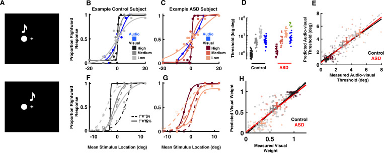
First, we probe whether individuals with ASD show a normal or impaired ability to optimally combine sensory cues across audio-visual pairings. To do so, individuals with ASD (n=31; mean ± S.E.M; 15.2±0.4 years; 5 females) and age-matched neurotypical controls (n=34, 16.1±0.4 years; 9 females) viewed a visual disk and/or heard an audio beep for 50 ms. The auditory tone and visual flash were synchronously presented either at the same location (Figure 1A, left panel) or separated by a small spatial disparity ∆ = ±6° (Figure 1A, right panel). The disparity was small enough to escape perceptual awareness (see explicit reports below for corroboration). The auditory stimulus was always the same, making the auditory signals equally reliable across trials. The reliability of the visual cue was manipulated by varying the size of the visual stimulus (see Methods for detail). On each trial, subjects indicated if the stimulus appeared to the right or left from straight ahead.

Figure 1. Audio-visual optimal cue combination in autism spectrum disorder (ASD).

Figure 1.

(A) Participants (neurotypical control or individual with ASD) viewed a visual disk and heard an auditory tone at different locations and with different small disparities (top = no disparity, bottom = small disparity). They had to indicate the location of the audio-visual event. (B) Rightward (from straight ahead) responses (y-axis) as a function of stimulus location (x-axis, positive = rightward) for an example, control subject. Color gradient (from darkest to lightest) indicates the reliability of the visual cue. (C) As (B), but for an example, ASD subject. (D) Discrimination thresholds in localizing audio (blue) or visual stimuli with different reliabilities (color gradient) for control (black) and ASD (red) subjects. Every point is an individual subject. A subset of six ASD subjects had very poor goodness of fit to a cumulative Gaussian (green) and were excluded from subsequent analyses. (E) Measured (x-axis) vs. predicted (y-axis) audio-visual discrimination threshold, as predicted by optimal cue integration. Black and red lines are the fit to all participants and reliabilities, respectively, for the control and ASD subjects. Two-dimensional error bars are the mean and 95% CI for each participant group and reliability condition. (F) Rightward response of an example control subject as a function of mean stimulus location (x-axis, auditory at +3 and visual –3 would result in mean stimulus location = 0) and disparity, the visual stimuli being either to the right (solid curve) or left (dashed) of the auditory stimuli. Color gradient shows the same gradient in reliability of the visual cue as in (B). (G) As (F), but for an example, ASD subject. (H) Measured (x-axis) vs. predicted (y-axis) visual weights, according to Equation 2 (Methods). Convention follows that established in (E). Both control (black) and ASD (red) subjects dynamically adjust the weight attributed to each sensory modality according to their relative reliability.

Figure 1B and C, respectively, shows the location discrimination of unisensory stimuli (audio in blue and visual according to a color gradient) for an example, control and ASD subject. Overall, subjects with ASD (6.83±0.68°) localized the visual stimulus as well as neurotypical subjects (6.30±0.49°, Figure 1D, no group effect, F[1, 57]=0.88, p=0.35, η2=0.01). As visual reliability decreased (lighter colors), the psychometric curves became flatter indicating larger spatial discrimination thresholds (high reliability: 1.10±0.07°, medium: 4.76±0.36°, low: 13.96±0.82°). This effect of visual reliability was equal across both subject groups (group × reliability interaction, F[2, 114]=0.11, p=0.89, η2<0.01), with visual thresholds being equal in control and ASD across all reliability levels. Auditory discrimination seemed to highlight potentially two subgroups within the ASD cohort (blue vs. green). Auditory threshold estimation was not possible for 6 of the 31 subjects within the ASD group (Figure 1D, green, R2 value <0.50), due to a lack of modulation in their reports as a function of cue location (excluding these 6 subjects, average R2 neurotypical control = 0.95; average R2 ASD = 0.96). Given that the central interest here is in interrogating audio-visual cue combination, and its agreement or disagreement with optimal models of cue combination, the rest of the analyses focuses on the 25 ASD subjects (and the control cohort) who were able to localize auditory tones. Auditory thresholds were similar across neurotypical controls and the ASD cohort where threshold estimation was possible (t57=–1.14, p=0.21, Cohen’s d=0.11).

The central hallmark of multisensory cue combination is the improvement in the precision of estimates (e.g. reduced discrimination thresholds) resulting from the integration of redundant signals. Optimal integration (Ernst and Banks, 2002) specifies exactly what ought to be the thresholds derived from integrating two cues, and thus we can compare measured and predicted audio-visual thresholds, according to optimal integration (see Equations 1; 2 in Methods). Figure 1E demonstrates that indeed both control (gradients of black) and ASD (gradients of red) subjects combined cues in line with predictions from statistical optimality (control, slope = 0.93, 95% CI = [0.85–1.04]; ASD, slope = 0.94, 95% CI = [0.88–1.08]). These results generalize previous findings from Zaidel et al., 2015 and suggest that across sensory pairings (e.g. audio-visual here, visuo-vestibular in Zaidel et al., 2015) statistically optimal integration of multisensory cues is intact in ASD.

A second characteristic of statistically optimal integration is the ability to dynamically alter the weight attributed to each sensory modality according to their relative reliability, i.e., decreasing the weight assigned to less reliable cues. Figure 1F and G, respectively, shows example psychometric functions for an example control and ASD individual when auditory and visual stimuli were separated by a small spatial disparity (Δ=±6°). Both show the same pattern. When the auditory stimulus was to the right of the visual stimulus (∆=6°, dashed curves), psychometric curves at high reliability (dark black and red symbols for control and ASD) were shifted to the right indicating a leftward bias, in the direction of the visual cue (see Methods). At low visual reliability, psychometric curves shifted to the left indicating a rightward bias, toward the auditory cue. That is, in line with predictions from optimal cue combination, psychometric curves shifted to indicate auditory or visual ‘dominance’, respectively, when auditory and visual cues were the most reliable. Analogous shifts of the psychometric functions were observed when the auditory stimulus was to the left of the visual stimulus (∆=−6°, solid curves). At the intermediary visual reliability – matching the reliability of auditory cues (Figure 1D) – both stimuli influenced localization performance about equally. Such a shift from visual to auditory dominance as the visual cue reliability worsened was prevalent across ASD and control subjects. Importantly, measured and predicted visual weights according to optimal cue combination were well matched in control (Figure 1H, black, slope = 0.97, 95% CI = [0.92–1.02]) and ASD (Figure 1H, red, slope = 0.99, 95% CI = [0.93–1.05]) groups. Measured visual weights were also not different between groups at any reliability (F[2, 114]=1.11, p=0.33, η2=0.02). Thus, just as their neurotypical counterparts, ASD subjects dynamically reweighted auditory and visual cues on a trial-by-trial basis depending on their relative reliabilities. Together, this pattern of results suggests that individuals with ASD did not show impairments in integrating perceptually congruent (and near-congruent) auditory and visual stimuli.

Impaired audio-visual causal inference

Having established that the process of integration is itself intact in ASD, we next queried implicit causal inference – the more general problem of establishing when cues ought to be integrated vs. segregated. Individuals with ASD (n=21, 17.32±0.57 years; 5 females) and age-matched neurotypical controls (n=15, 16.86±0.55 years; 7 females, see Supplementary file 1, Supplementary file 2 for overlap in cohorts across experiments) discriminated the location of an auditory tone (50 ms), while a visual disk was presented synchronously at varying spatial disparities. The stimuli were identical to those above but spanned a larger disparity range (∆=±3,±6,±12, and ±24°), including those large enough to be perceived as separate events (see explicit reports below). Subjects indicated if the auditory stimulus was located to the left or right of straight ahead, and as above, we fit psychometric curves to estimate perceptual biases. The addition of large audio-visual disparities fundamentally changes the nature of the experiment, where now observers must first ascertain an internal model, i.e., whether auditory and visual cues come from the same or separate world sources. As the disparity between cues increases, we first expect to see the emergence of perceptual biases – one cue influencing the localization of the other. However, as cue disparities continue to increase, we expect observers to switch worldviews, from a regime where cues are hypothesized to come from the same source, to one where cues are now hypothesized to come from separate sources. Thus, as cue disparities continue to increase, eventually the conflict between cues ought to be large enough that perceptual biases asymptote or decrease, given that the observer is operating under the correct internal model (Körding et al., 2007; Rohe and Noppeney, 2015; Rohe and Noppeney, 2016; Rohe et al., 2019; Cao et al., 2019; Noel and Angelaki, 2022).

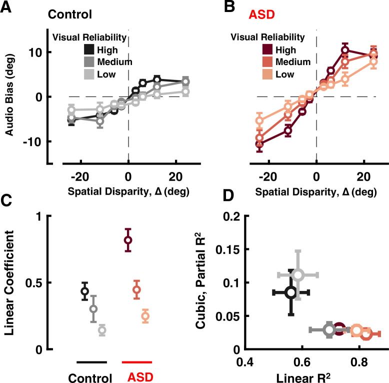
Overall, individuals with ASD showed a larger bias (i.e. absolute value of the mean of the cumulative Gaussian fit) in auditory localization than the control group (see Figure 2A and B, respectively, for control and ASD cohorts; F[1, 34]=5.44, p=0.025, η2=0.13). Further, how the bias varied with spatial disparity (∆) significantly differed between the groups (group × disparity interaction: F[7, 168]=3.50, p=0.002, η2=0.12). While the bias saturated at higher ∆ in neurotypical subjects, as expected under causal inference, the bias increased monotonically as ∆ increased in the ASD group. Thus, despite increasing spatial discrepancy, ASD subjects tended to integrate the cues, as if they nearly always utilized visual signals to localize the auditory cue and did not readily switch to a worldview where the auditory and visual cues did not come from the same world source. The effect of visual cue reliability was similar in both groups (group × reliability interaction, F[2, 168]=1.05, p=0.35, η2=0.01), indicating that the auditory bias decreased as visual cue reliability worsened in both groups.

Figure 2. Audio-visual causal inference.

Participants (black = control; ASD = red) localized auditory tones relative to straight ahead, in the presence of visual cues at different disparities of up to 24°. See Supplementary file 1, Supplementary file 2 for overlap of subjects with Figure 1. (A) Auditory bias (y-axis, central point of the cumulative Gaussian, e.g. Figure 1B) as a function of spatial disparity (x-axis, relative location of the visual cue) and reliability of the visual cue (darker = more reliable) in control subjects. (B) As (A), but for individuals with ASD. (C) Coefficient of the linear fits (y-axis, larger value indicates quicker increase in bias with relative visual location) in control (black) and ASD (red), as a function of visual cue reliability (darker = more reliable). (D) Linear R2 (x-axis) demonstrates that the linear fits account well for observed ASD data. On the other hand, adding a cubic term (y-axis, partial R2) improved fit to control data (at two reliabilities) but not ASD data. Error bars are ±1 S.E.M.

Figure 2.

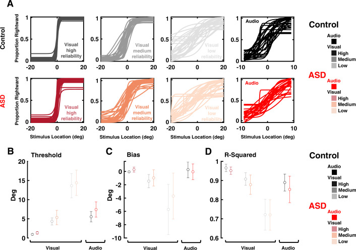
Figure 2—figure supplement 1. Visual and auditory localization performance of participants in Experiment 2 (audio-visual implicit causal inference).

Figure 2—figure supplement 1.

(A) Proportion of ‘rightward’ report as a function of stimulus location (in deg, x-axis, positive values indicate the right hemifield). Top row: all control subjects. From left to right: visual discrimination at high, medium, and low reliability, and finally auditory discrimination. Bottom row: as top row, for all autism spectrum disorder (ASD) subjects. (B) Discrimination thresholds for ASD and controls subjects, for low, medium, and high reliability visual stimuli, as well as auditory cues. Dots and error bars are the mean and S.E.M for each group and condition. (C) and (D) are, respectively, the bias and R-squared. Format follows that of (B). Results indicate that psychometric thresholds (all p>0.09), bias (all p>0.11), and goodness of fit (all p>0.26) are not different across the ASD and control cohorts, across visual and auditory modalities, and across all reliabilities.
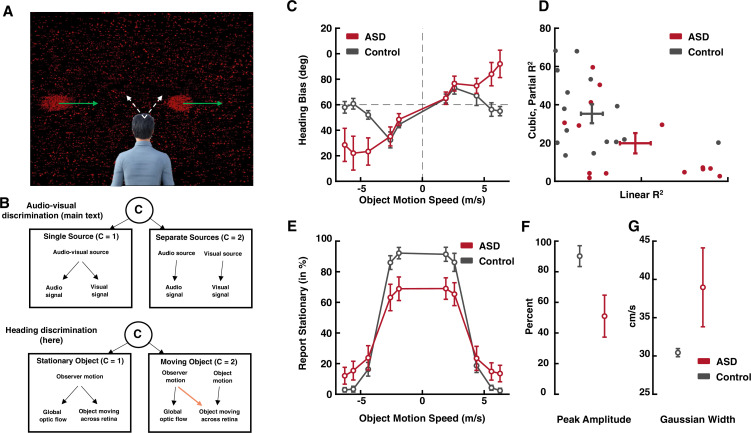
Figure 2—figure supplement 2. Heading discrimination during concurrent implied self-motion and object motion.

Figure 2—figure supplement 2.

We very briefly present these results, as a conceptual replication and extension of the main audio-visual results, in order to highlight the statistical reliability and generalizability of the main result – an internal model most readily specifying integration in autism spectrum disorder (ASD). (A) Subjects are presented with a wide field of dots (background) that move as to imply self-motion, leftward or rightward, at different angles (white arrows). Simultaneously, an object (red clouds of dots) may move independently, at different speeds. Observers are asked to report on their own self-motion by button press (either leftward or rightward from straight-ahead), as well as to indicate if the object moved or not. (B) This task requires causal inference in attributing motion across our retinas to self-motion or object-motion, yet the generative model is distinct (c.f. orange arrow) from that reported in the main text (audio-visual). (C) Heading bias as a function of object motion speed. As predicted by causal inference, the control group (black), shows a bias peaking at intermediary cue disparities, which then dissipates as the observer infers two separate causes (see Dokka et al., 2019). Instead, the ASD group (dark red) shows a monotonically increasing bias, as if always integrating cues. (D) Linear fits account better for ASD than control data (x-axis), while adding a cubic component to the regression aids in explaining control but not ASD data. (E) Reports of the object being stationary, as a function of its speed in the world. As expected, reports of stationarity occur more often when the object moves at a slow speed. The peak report of stationarity in ASD is lower than that of control subjects (F), and the velocity range over which reports of stationarity are likely, is larger in ASD than control individuals (G). Dots are means, and error bars are ±1 S.E.M.

To more rigorously quantify how auditory localization depended on ∆, we fit a third-order regression model to the auditory bias as a function of ∆, independently for each subject and at each visual reliability (y=a0+a1∆+a22+a33; see Methods). As shown in Figure 2C, across all visual reliabilities, the ASD group had a larger linear coefficient (a1, ANOVA: F[1, 34]=6.69, p=0.014, η2=0.16), again indicating a monotonic increase in bias with cue spatial disparity.

To better account for putative non-linear effects at large ∆ - those which ought to most clearly index a change from integration to segregation - we fit different regression models (i.e. null, linear, quadratic, and cubic) and estimated the added variance accounted by adding a cubic term (partial R2). This latter term may account for non-linear effects at large ∆, where the impact of visual stimuli on auditory localization may saturate or even decrease (a3 being zero or negative) at large disparities. Results showed that not only the linear term accounted for more variance in the ASD data than controls (Figure 2D and x-axis, ANOVA: F[1, 34]=7.08, p=0.012, η2=0.17), but also the addition of a cubic term significantly improved fits in the control, but not ASD, group (Figure 2D and y-axis, partial R2, ANOVA: F[1, 34]=9.87, p=0.003, η2=0.22). Taken together, these results suggest that contrary to predictions from causal inference – where disparate cues should affect one another at small but not large disparities, i.e., only when they may reasonably index the same source – ASD subjects were not able to down-weight the impact of visual cues on auditory localization at large spatial disparities, resulting in larger errors in auditory localization.

To confirm that the larger biases observed within the ASD cohort were in fact due to these subjects using an incorrect internal model, and not a general impairment in cue localization, we compared unisensory visual and auditory localization thresholds and biases between experimental groups. From the 21 ASD and 15 control subjects who participated in the audio-visual causal inference experiment (Experiment 2), respectively, 15 and 14 of these also participated in Experiment 1 - performing an auditory and visual localization experiment with no disparity (see Supplementary file 1, Supplementary file 2 for further detail). Figure 2—figure supplement 1A shows the psychometric functions (auditory localization and visual localization at three different reliability levels) for all subjects participating in Experiment 2. Psychometric thresholds (Figure 2—figure supplement 1B, all p>0.09), bias (Figure 2—figure supplement 1C, all p>0.11), and goodness of fit (Figure 2—figure supplement 1D, all p>0.26) were not significantly different between the ASD and control cohorts, across visual and auditory modalities, and across all reliabilities.

Last, to further bolster the conclusion that individuals with ASD show anomalous implicit causal inference, we replicate the same effect in a very different experimental setup. Namely, subjects (n=17 controls, n=14 ASD, see Supplementary file 1, Supplementary file 2) performed a visual heading discrimination task requiring the attribution of optic flow signals to self-motion and/or object-motion (a causal inference task requiring the attribution of motion across the retina to multiple sources, self and/or object; see Dokka et al., 2019, Methods, and Figure 2—figure supplement 2A for further detail). We describe the details in the Supplementary materials given that the task is not audio-visual and has a different generative model (Figure 2—figure supplement 2B). Importantly, however, the results demonstrate that while heading biases are present during intermediate self-velocity disparities and object-velocity disparities for controls and ASD subjects (Figure 2—figure supplement 2C, D), they disappear during large cue discrepancies in control subjects, but not ASD subjects. Just as in the audio-visual case (Figure 2), ASD subjects do not readily change worldviews and move from integration to segregation as disparities increase (Figure 2—figure supplement 2C, D).

Together, these results suggest that in ASD the process of integrating information across modalities is normal (see Zaidel et al., 2015) once a correct internal model of the causal structure of the world has been formed. However, the process of inferring this causal structure – the set of relations between hidden sources and sensory signals that may have given rise to the observed data – is anomalous. Namely, individuals with ASD seem to operate under the assumption that sensory cues ought to be integrated most of the time, even for large disparities. Next, we questioned if and how this deficit in causal inference expresses explicitly in overt reports.

Decreased disparity-independent explicit report of common cause

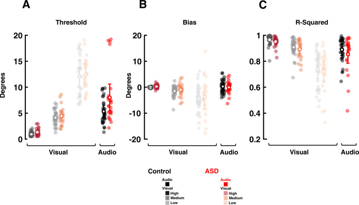
Individuals with ASD (n=23; 16.14±0.51 years; 5 females) and age-matched neurotypical controls (n=24; 17.10±0.42 years; 7 females; see Supplementary file 1, Supplementary file 2 for overlap in cohorts with previous experiments) viewed a visual disk and heard an auditory tone presented synchronously (50 ms), but at different spatial disparities (same stimuli as above, disparity up to 24°). Participants indicated whether the auditory and visual cues originated from a common source, or from two separate sources (see Methods for instructions). In contrast to the localization experiments, where subjects localized the physical position of stimuli, here subjects were asked to explicitly report the relationship between the auditory and visual stimuli. See Figure 3—figure supplement 1 for the unisensory discrimination performance in participants who took part in both the cue integration experiment (Experiment 1) and the current explicit common cause report across spatial disparities. Auditory and visual localization thresholds (all p>0.07), bias (all p>0.15), and the goodness of fit (all p>0.16) of these psychometric estimates were no different between the ASD and control cohort participating in this explicit causal inference judgment experiment.

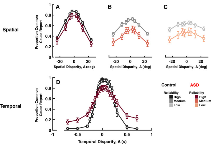
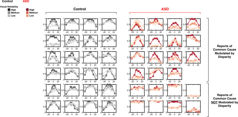
As expected, most subjects reported a common source more frequently at smaller rather than larger ∆ (Figure 3 F[8, 259]=94.86, p<0.001, η2=0.74). Interestingly, while this pattern was true for all individual control subjects, eight of the individuals with ASD (i.e. ~⅓ of the cohort) did not modulate their explicit common cause reports as a function of spatial disparity, despite good auditory and visual localization (see Figure 3—figure supplement 1 and Figure 3—figure supplement 2). These subjects were not included in subsequent analyses. For lower visual reliability (Figure 3, from A-C), both groups reported common cause less frequently (F[2, 74]=10.68, p<0.001, η2=0.22). A striking difference between experimental groups was the decreased likelihood of reporting common cause, across spatial disparities and visual cue reliabilities, in ASD relative to controls (Figure 3A–C shades of black vs. shades of red, F[1, 37]=11.6, p=0.002, η2=0.23). This pattern of results using an explicit causal inference task is opposite from that described for the implicit task of auditory localization, where individuals with ASD were more, and not less, likely to combine cues.

Figure 3. Explicit common cause reports across spatial (top) and temporal (bottom) disparities.

Proportion of common cause reports (y-axis) as a function of spatial disparity (x-axis) and visual cue reliability; high (A), medium (B), or low (C). The most striking characteristic is the reduced likelihood to report common cause, across any disparity or cue reliability. (D) Proportion of common cause reports (y-axis) as a function of temporal disparity. As indexed by many (e.g. Feldman et al., 2018) individuals with autism spectrum disorder (ASD) show larger ‘temporal binding windows’; temporal extent over which they are likely to report common cause. However, these individuals are also less likely to report common cause, when auditory and visual stimuli are in very close temporal proximity (an effect sometimes reported, e.g., Noel et al., 2018b, but many times neglected, given normalization from 0 to 1, to index binding windows; see e.g., Woynaroski et al., 2013; Dunham et al., 2020). See Supplementary file 1, Supplementary file 2 for overlap of subjects with previous figures. Error bars are ±1 S.E.M.

Figure 3.

Figure 3—figure supplement 1. Visual and auditory localization performance of participants in Experiment 3 (audio-visual explicit causal inference).

Figure 3—figure supplement 1.

A) Discrimination thresholds for autism spectrum disorder (ASD) and controls subjects, for low, medium, and high reliability visual stimuli, as well as auditory cues. Transparent dots are individual subjects, while opaque white circles and error bars are mean and S.E.M. (B) and (C) follow the formatting of (A), but respectively, show the bias and R-squared. Four ASD subjects had poor auditory localization performance (as seen in the threshold and R-squared subplots) yet even including these subjects did not differentiate between ASD and control cohorts in threshold, bias, or R-squared.
Figure 3—figure supplement 2. Reports of common cause as a function of spatial disparity.

Figure 3—figure supplement 2.

All individual data is presented. Report of ‘common cause’ (y-axis) as a function of spatial disparity (x-axis) and visual reliability (color gradient). Data of all control subjects (first to fourth column) are modulated by disparity. 15/23 Autism spectrum disorder (ASD) subjects (top four rows of columns five to eight) showed a modulation in explicit reports of common cause by disparity. However, 8 (bottom two rows) did not.
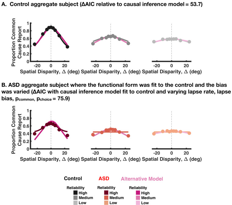
Figure 3—figure supplement 3. Fitting a functional form to the explicit causal inference reports.

Figure 3—figure supplement 3.

(A) We fit a functional model of the form a*N(X;mu,sd^2)+b where X is the spatial disparity. The model was fit for each reliability therefore with 12 parameters in total. The model predictions are shown in shades of magenta with the causal inference model predictions in gray. The causal inference model performs better than the functional form as quantified by Akaike Information Criterion (AIC) as indicated in the title. (B) The functional form in (A) was fit to control subjects and then the bias (parameter ‘b’ in the equation) was varied to best explain the autism spectrum disorder (ASD) subject responses. This model was outperformed (quantified by AIC) by the causal inference model, which was also fit to the control subjects with choice and inference parameters varied.

These differences were quantified by fitting Gaussian functions to the proportion of common source reports as a function of ∆ (excluding the eight ASD subjects with no modulation in their reports; R2 for this cohort <0.5). The Gaussian fits (control: R2=0.89±0.02; ASD: R2=0.93±0.01) yield three parameters that characterize subjects’ behavior: (1) peak amplitude, which represents the maximum proportion of common source reports; (2) mean, which represents the ∆ at which subjects perceived a common source most frequently; and (3) width (SD), which represents the range of ∆ over which the participant was likely to perceive a common source. Both control and ASD participants perceived a common source most frequently at a ∆ close to 0°, and there was no group difference for this parameter (control = 0.30±1.33°; ASD = 0.48±1.9°; F[1, 37]<0.01, p=0.92, η2<0.01). Amplitude and width, however, differed between the two groups. The peak amplitude of the best-fit Gaussian was smaller for the ASD than the control group (control = 0.75±0.02; ASD = 0.62±0.05; F[1, 37]=8.44, p=0.0006, η2=0.18), quantifying the fact that the ASD group perceived a common source less frequently than control participants. The width of the Gaussian fit was smaller in the ASD compared to the control group (control = 30.21±2.10°; ASD = 22.35±3.14°; F[1, 37]=7.00, p=0.012, η2=0.15), suggesting that the range of spatial disparities at which ASD participants perceived a common source was significantly smaller than in controls. Note, this range is well beyond the 6° used in the maximum likelihood estimation experiment (~fourfold), thus corroborating that during the first experiment participants perceived auditory and visual cues as a single, multisensory cue.

To further substantiate these differences in the explicit report of common cause across ASD and neurotypical subjects, we next dissociated auditory and visual cues across time, as opposed to space. Twenty-one individuals with ASD (15.94±0.56 years; 5 females) and 13 age-matched neurotypical controls (16.3±0.47 years; 5 females, see Supplementary file 1, Supplementary file 2) viewed a visual disk and heard an auditory tone, either in synchrony (∆=0 ms) or over a wide range of asynchronies (from ±10 to ±700 ms; positive ∆ indicates visual led auditory stimulus). Subjects indicated if auditory and visual stimuli occurred synchronously or asynchronously.

Analogous to the case of spatial disparities, we fit reports of common cause (i.e. synchrony, in this case) to Gaussian functions. Just as for spatial disparities, the ASD group had smaller amplitudes (ASD = 0.83±0.04; control = 0.98±0.01; Figure 3D; t-test: t32=7.75, p<0.001, Cohen’s d>2), suggesting that at small ∆ individuals with ASD perceived the stimuli as originating from a common cause less frequently than control subjects did. Further, the ASD group exhibited larger Gaussian widths (control = 171.68±13.17; ASD = 363±55.63 ms; t-test: t32=2.61, p=0.01, Cohen’s d=0.9), reflecting more frequent reports of common cause at large temporal disparities. This second effect corroborates a multitude of reports demonstrating larger ‘temporal binding windows’ in ASD than control (see Feldman et al., 2018 for a meta-analysis of 53 studies). Overall, therefore, explicit reports of common cause across spatial and temporal disparities agree in suggesting a lower likelihood of inferring a common cause at small temporal disparities - including no disparity - in ASD relative to neurotypical controls (see e.g. Noel et al., 2018b; Noel et al., 2018a, for previous reports showing altered overall tendency to report common cause during temporal disparities in ASD, although these reports typically focus on the size of ‘binding windows’).

Correlational analyses between psychometric features distinguishing control and ASD individuals (i.e. linear and cubic terms accounting for auditory biases during large audio-visual spatial disparities, amplitude and width of explicit common cause reports during spatial and temporal disparities) and symptomatology measures, i.e., autism quotient (AQ; Baron-Cohen et al., 2001) and social communication questionnaire (SCQ; Rutter et al., 2003) demonstrated weak to no association. Of the 12 correlations attempted ([AQ + SCQ] × [amplitude + width] × [temporal + spatial] + [AQ + SCQ] × [linear + cubic terms]), the only significant relation (surviving Bonferroni-correction) was that between the width of the Gaussian function describing synchrony judgments as a function of temporal disparity and SCQ scores (Type II regression: r=0.52, p=0.002; see Smith et al., 2017 for a similar observation).

Causal inference modeling suggests an increased prior probability for common cause in ASD

To bridge across experiments (i.e. implicit and explicit audio-visual spatial tasks) and provide a quantitative account of the switch between internal models (i.e. segregate vs. integrate) in ASD vs. controls, we fit subjects’ responses with a Bayesian causal inference model (Figure 4A and Körding et al., 2007). The modeling effort is split in three steps.

Figure 4. Causal inference modeling of implicit and explicit spatial tasks.

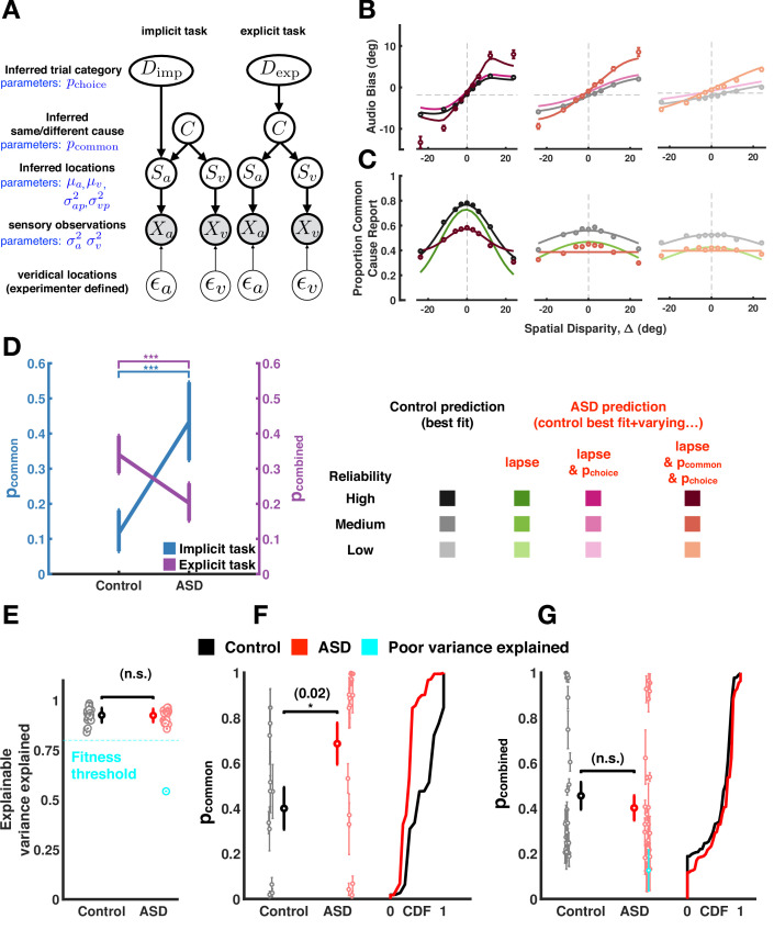
(A) Generative models of the causal inference process in the two tasks (implicit task in left and explicit task in right). The subject makes noisy sensory measurements (X) of the veridical cue locations (ϵ) and combines them with their prior belief to obtain their percept (S). To do so optimally, the subject first must infer whether signals came from the same cause (C) and thereby determine if it is useful to combine the information from the two cues for inferring the trial category (D). The causal inference process is shared between the two tasks but the subject infers Dimp (side of the tone) in the implicit task and Dexp (number of causes for the sensory observations) in the explicit task. (B) Aggregate data (dots) and model fits (lines) in the implicit task (the visual reliability varies from high to low from left to right). The causal inference model is fit to the control aggregate subject and different set of parameters are varied to match the autism spectrum disorder (ASD) subject data (see main text). See Figure 4—figure supplement 12 for a fit to the same data while (1) allowing all parameters free to vary, (2) allowing the same parameter as here to vary, but fitting to visual reliabilities separately, or (3) doing both (1) and (2). Of course, these result in better fits, but this is at the expense of interpretability in that they are inconsistent with the empirical data. (C) Same as (B) but fits are to the explicit spatial task. See Figure 4—figure supplement 13 for the equivalent of Figure 4—figure supplement 12, for the implicit task. Data (dots) are slightly different from that in Figures 2 and 3 because in the previous figures data was first averaged within subjects, then psychometric functions were fit, and finally estimates of bias were averaged across subjects. Here, data is first aggregated across all subjects and then psychometric fits are done on the aggregate. Importantly, the difference between ASD and control subjects holds either way. Error bars are 68% CI (see Supplementary file 4 for additional detail regarding deriving CIs for the amalgamated subject). (D). ASD subjects have a higher p-common for the aggregate subject in the implicit task but seemingly compensate in the explicit task where they show a lower aggregate p-common and choice bias. (E). The causal inference model provides an equally good fit (quantified by explainable variance explained), a measure of goodness of fit appropriate for noisy, as opposed to noiseless data (Haefner and Cumming, 2008) for control and ASD subjects. (F) Individual ASD (red) subjects have a higher p-common on average for the implicit task (in agreement with the aggregate subject) but (G) show no significant difference in the combined p-common and choice bias for the explicit task due to considerable heterogeneity across subjects. Subjects were included in the single-subject modeling effort if they had participated in Experiment 1 (and thus we had an estimate of their sensory encoding) in addition to the particular task of interest. That is, for panel (F), we included all participants taking part in Experiments 1 and 2. This included participants deemed poor in Experiment 1, given our attempt to account for participant’s behavior with the causal inference model. For panel (G), we included all participants taking part in Experiments 1 and 3. Individual subject error bars are 68% CI, while group-level error bars are 95% CI (see Supplementary file 4 for additional detail regarding statistical testing). CDF = cumulative density function.

Figure 4.

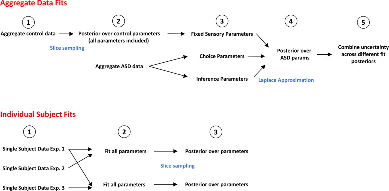
Figure 4—figure supplement 1. Flowchart detailing steps in fitting procedure.

Figure 4—figure supplement 1.

Top: Fit to aggregate data presented in Figure 4B,C and D. First, we aggregate the control data (1) and estimate posteriors for all parameters in order to best fit the data via slice sampling (2). Next, we attempt to account for the aggregate autism spectrum disorder (ASD) data while fixing the sensory parameters but varying choice and/or inference parameters (3). The empirical data suggests no difference in the sensory parameters between control and ASD (Figure 2—figure supplement 1, Figure 3—figure supplement 1), and including these parameters or allowing them to be free while the inference parameters are not, does not account well for the implicit data (Figure 4—figure supplement 7, Alternative A and B). Next, we estimate the posterior parameters for the ASD cohort (4, 5). Bottom: Fit to the single subject data presented in Figure 4F and G. For each participant data from Experiment 1 (allowing estimation of sensory parameters) and either Experiment 2 (implicit causal inference) or Experiment 3 (explicit causal inference in space) are aggregated (1). Then we fit all parameters in order to best account for the data (2) and estimate posteriors over these parameters by slice sampling (3).
Figure 4—figure supplement 2. Fit to aggregate data for the implicit causal inference task, allowing sensory uncertainty and choice parameters to vary but fixing the inference parameter pcommon (shown in pink).

Figure 4—figure supplement 2.

This model performs worse (quantified by Akaike Information Criterion [AIC] where positive AIC indicates worse fit) as compared to the model in the main paper where pcommon and the choice parameters are allowed to vary (shown in red).
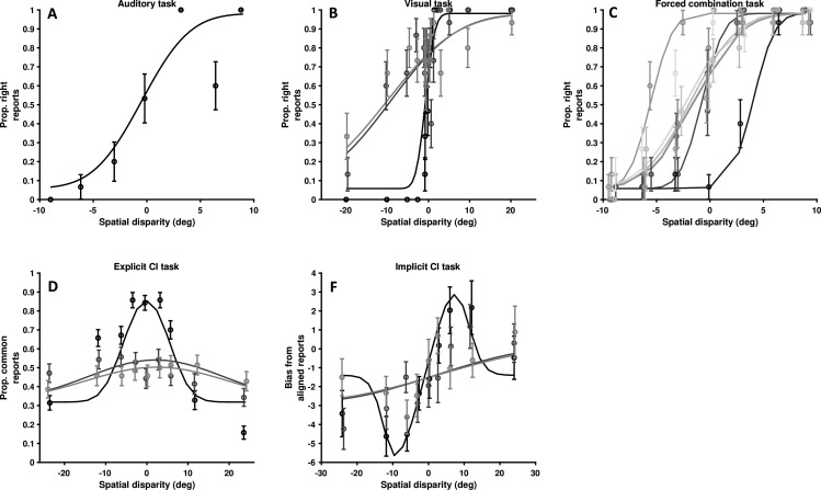
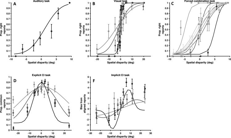
Figure 4—figure supplement 3. Data from a single, representative control subject.

Figure 4—figure supplement 3.

(A) Auditory localization, proportion rightward (y-axis) as a function of auditory position vis-à-vis straight ahead (x-axis, positive values are rightward). (B) Visual localization across three reliabilities levels, from high reliability in dark, to low reliability in light gray. Follows the format from A. (C) Forced fusion task, where auditory and visual cues are presented congruently or with a slight disparity (±6°). (D) Explicit causal inference task, where participants report whether auditory and visual cues originated from the same source (y-axis), according to different spatial disparities (x-axis) and visual reliability levels (darker = more reliable). (F) Implicit causal inference. Auditory bias (y-axis, in degree) as a function of audio-visual disparity (x-axis, up to 24° ) and visual reliability (darker = more reliable). Errors bars are ±1 S.E. The parameters of the causal inference model are simultaneously fit to all tasks, considerable constraining the model estimates.
Figure 4—figure supplement 4. Data from another single, representative control subject.

Figure 4—figure supplement 4.

As Figure 4—figure supplement 3, for a second representative control subject. (A) Auditory localization, proportion rightward (y-axis) as a function of auditory position vis-à-vis straight ahead (x-axis, positive values are rightward). (B) Visual localization across three reliability levels, from high reliability in dark, to low reliability in light gray. Follows the format from A. (C) Forced fusion task, where auditory and visual cues are presented congruently or with a slight disparity (±6°). (D) Explicit causal inference task, where participants report whether auditory and visual cues originated from the same source (y-axis), according to different spatial disparities (x-axis) and visual reliability levels (darker = more reliable). (F) Implicit causal inference. Auditory bias (y-axis, in degree) as a function of audio-visual disparity (x-axis, up to 24°) and visual reliability (darker = more reliable). Errors bars are ±1 S.E. The parameters of the causal inference model are simultaneously fit to all tasks, considerable constraining the model estimates.
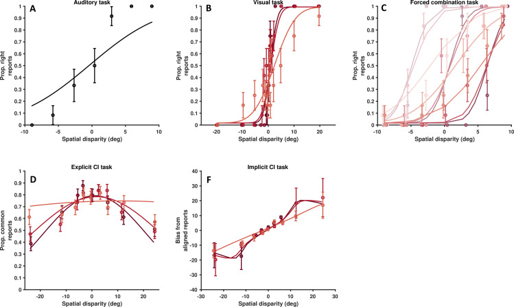
Figure 4—figure supplement 5. Data from a single, representative autism spectrum disorder (ASD) subject.

Figure 4—figure supplement 5.

As Figure 4—figure supplements 3 and 4, for a representative ASD subject. (A) Auditory localization, proportion rightward (y-axis) as a function of auditory position vis-à-vis straight ahead (x-axis, positive values are rightward). (B) Visual localization across three reliability levels, from high reliability in dark, to low reliability in light gray. Follows the format from A. (C) Forced fusion task, where auditory and visual cues are presented congruently or with a slight disparity (±6°). (D) Explicit causal inference task, where participants report whether auditory and visual cues originated from the same source (y-axis), according to different spatial disparities (x-axis) and visual reliability levels (darker = more reliable). (F) Implicit causal inference. Auditory bias (y-axis, in degree) as a function of audio-visual disparity (x-axis, up to 24°) and visual reliability (darker = more reliable). Errors bars are ±1 S.E. The parameters of the causal inference model are simultaneously fit to all tasks, considerable constraining the model estimates.
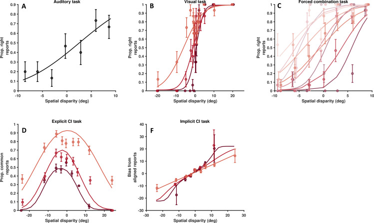
Figure 4—figure supplement 6. Data from another single, representative autism spectrum disorder subject.

Figure 4—figure supplement 6.

As Figure 4—figure supplement 5, for a second representative control subject. (A) Auditory localization, proportion rightward (y-axis) as a function of auditory position vis-à-vis straight ahead (x-axis, positive values are rightward). (B) Visual localization across three reliabilities levels, from high reliability in dark, to low reliability in light gray. Follows the format from A. (C) Forced fusion task, where auditory and visual cues are presented congruently or with a slight disparity (±6°). (D) Explicit causal inference task, where participants report whether auditory and visual cues originated from the same source (y-axis), according to different spatial disparities (x-axis) and visual reliability levels (darker = more reliable). (F) Implicit causal inference. Auditory bias (y-axis, in degree) as a function of audio-visual disparity (x-axis, up to 24°) and visual reliability (darker = more reliable). Errors bars are ±1 S.E. The parameters of the causal inference model are simultaneously fit to all tasks, considerable constraining the model estimates.
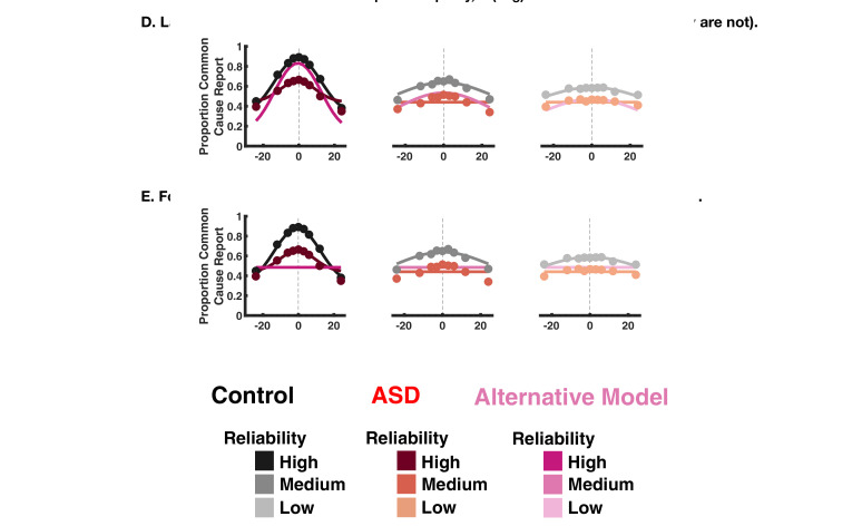
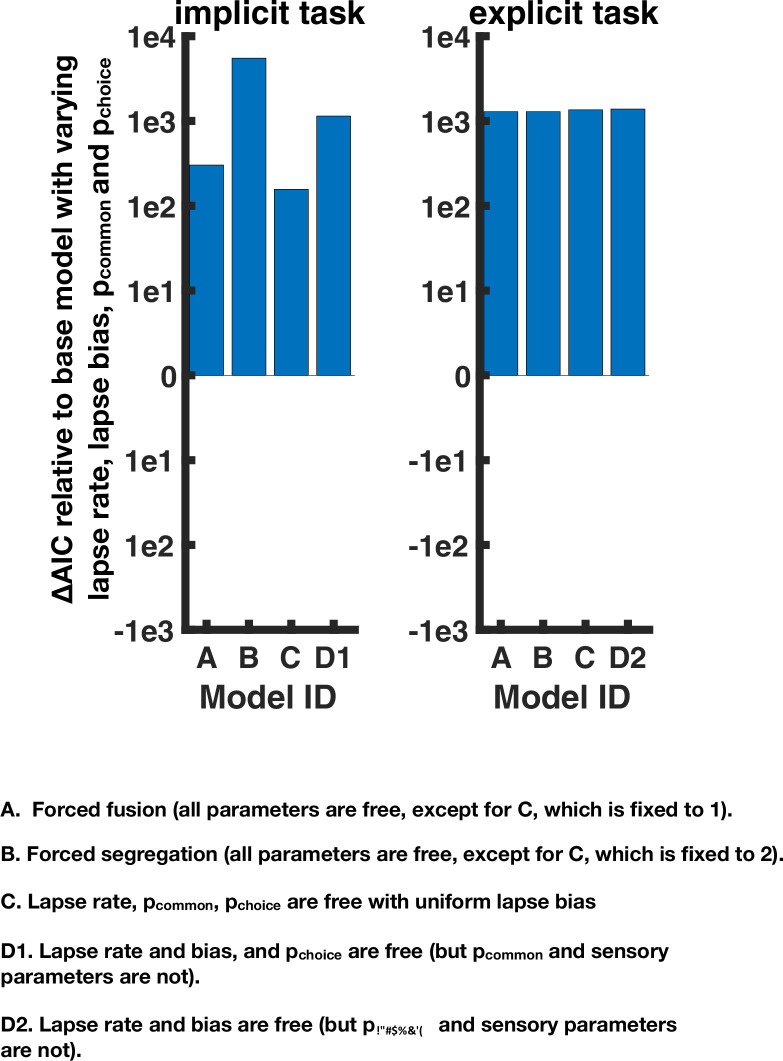
Figure 4—figure supplement 7. Goodness of fit of alternative models for the implicit and explicit spatial causal inference task.

Figure 4—figure supplement 7.

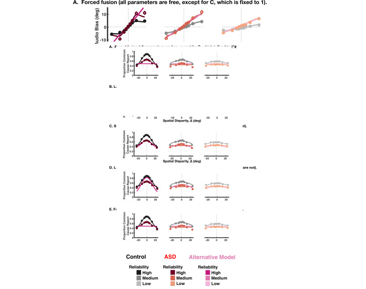
Four alternatives were tested: (A) a forced fusion model where C is set to 1. (B) A forced segregation model where C is set to 2. (C) A model where there is no lapse bias. (D1) An alternative where solely choice parameters are varied for implicit task: the lapse parameters and pchoice (D2). For the explicit task, pchoice cannot be separately constrained from pcommon so only the lapse parameters are varied. For the implicit task, two main observations must be noted. First, all models perform worse than that presented in the main text (y-axis is difference to the model presented in the main text, with higher Akaike Information Criterion [AIC] indicating a worse quality of fit). Second, Alternative A is substantially better than Alternative B, but still worse than the model in the main text. Thus, seemingly individuals with autism spectrum disorder do perform causal inference and not pure forced fusion, yet they overweight integration (vs. segregation) compared to their neurotypical counterparts. For the explicit task, all alternative models perform worse than the model in the main text where the choice and inference parameters were varied.
Figure 4—figure supplement 8. Illustration of the alternative models fits to implicit causal inference model data.

Figure 4—figure supplement 8.

The rows show the four alternative models tested, while the columns show data in decreasing order of reliability. For each panel, the model presented in the main text is shown, in shades of black for the control subjects and shades of red for the autism spectrum disorder subjects. The alternative tested in each panel is shown in shades of magenta.
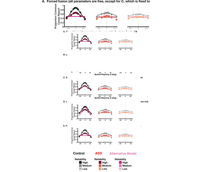
Figure 4—figure supplement 9. Illustration of the alternative models fits to explicit causal inference model data.

Figure 4—figure supplement 9.

The rows show the four alternative models tested, while the columns show data in decreasing order of reliability. For each panel, the model presented in the main text is shown, in shades of black for the control subjects and shades of red for the autism spectrum disorder subjects. The alternative tested in each panel is shown in shades of magenta.
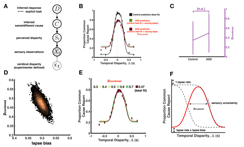
Figure 4—figure supplement 10. Causal inference modeling of temporal, simultaneity judgment task.

Figure 4—figure supplement 10.

(A) Causal inference model for auditory-visual simultaneity judgement. This model is a simplified version from the full model in Figure 4A by measuring temporal judgments relative to a reference cue (the auditory cue in this case). (B) Model fits to aggregate subjects in the explicit temporal task. The causal inference model is fit to the control aggregate subject and different set of parameters are varied to match the autism spectrum disorder (ASD) subject data (similar to Figure 4). (C) Estimated pcombined cannot be accurately constrained using the given data, as illustrated by the large error bars. (D) Scatter plots of samples from the joint posterior distribution between the pcombined parameter and the lapse bias parameter. The two parameters are (negatively) correlated (r=−0.72) making them hard to separate. (E) Illustration of the correlation between the parameters in B. Fixing the pcombined to a range of values between 0.3 and 0.7, we can estimate the lapses such that the model provides a qualitatively good prediction to the data, hence making it hard to constrain the pcombined as seen in C. (F) The predicted responses from the causal inference model can be visualized as a difference between two cumulative Gaussian functions with a vertical scaling and offset determined by the lapse rate and lapse biases. The slope of the cumulative Gaussian is a function of the sensory uncertainty, whereas the separation is a function of pcombined. By fixing the slope, offset, and scaling from the sensory uncertainties and lapses, the differences between the curves for different pcombined are small, making it hard to separate using reasonable amount of empirical data.
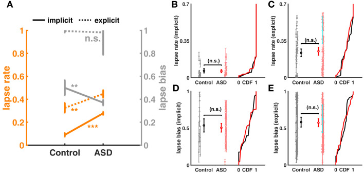
Figure 4—figure supplement 11. Lapse rate and lapse bias for aggregate and individual subjects during the implicit and explicit spatial tasks.

Figure 4—figure supplement 11.

(A) Aggregate lapse rate and lapse bias for controls and autism spectrum disorder (ASD) (plotted similar to main text Figure 4D). We find that in both implicit and explicit causal inference tasks, ASD subjects have a higher lapse rate. ASD subjects also seem to have a larger deviation from a uniform lapse bias of 0.5. (B–D) Lapse rate and lapse bias fit to individual subjects. There is no significant difference in the lapse rate and lapse bias for both tasks due to considerable heterogeneity across subjects. Subject depictured in blue is the same as in Figure 4, main text.
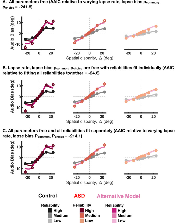
Figure 4—figure supplement 12. Fit to aggregate data for the implicit causal inference task, given that all parameters are free to vary (A), the different visual reliabilities are fit separately (B) or both of the above (C).

Figure 4—figure supplement 12.

The change in Akaike Information Criterions (AICs) is reported in the panel title, with all values being smaller than the baseline model, suggesting better fits. Shades of black and red are, respectively, the baseline model for control and autism spectrum disorder (ASD) subjects, while shades of magenta are the comparison model.
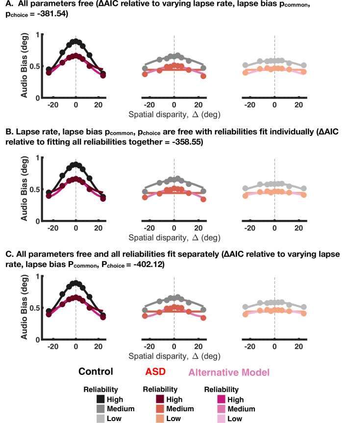
Figure 4—figure supplement 13. Fit to aggregate data for the explicit causal inference task, given that all parameters are free to vary (A), the different visual reliabilities are fit separately (B) or both of the above (C).

Figure 4—figure supplement 13.

The change in Akaike Information Criterions (AICs) is reported in the panel title, with all values being smaller than the baseline model, suggesting better fits. Shades of black and red are, respectively, the baseline model for control and autism spectrum disorder (ASD) subjects, while shades of magenta are the comparison model.

First, we fit aggregate data and attempt to discern which of the parameters that govern the causal inference process may globally differ between the ASD and control cohorts. The parameters of the causal inference model can be divided into three sets. First, sensory parameters: the visual and auditory sensory uncertainty (i.e. inverse of reliability), as well as visual and auditory priors (i.e. expectations) over the perceived auditory and visual locations (mean and variance of Gaussian priors). Second, choice parameters: choice bias (pchoice), as well as lapse rate and bias. These latter two parameters are the frequency with which an observer may make a choice independent of the sensory evidence (lapse rate) and whether these stimuli-independent judgments are biased (lapse bias). Third, inference parameters: the prior probability of combination (pcommon; see Methods and Supplementary file 3, Supplementary file 4 for further detail). In this first modeling step, we fit all parameters (see Supplementary file 3) to best account for the aggregate control subject. Then, we test whether a difference in choice and inference parameters, but not the sensory ones, can explain the observed difference between the control and the aggregate ASD data. We do not vary the sensory parameters given that unisensory discrimination thresholds did not differ between experimental groups (Figure 1, Figure 2—figure supplement 1, and Figure 3—figure supplement 1. See Methods, Supplementary file 4 and Figure 4—figure supplement 1 for technical detail regarding the model fitting procedure. Also see Figure 4—figure supplement 2 corroborating the fact that varying the inference parameter, as opposed to sensory uncertainty, results in better model fits). In a second step, we attempt not to globally differentiate between ASD and control cohorts, but to account for individual subject behavior. Thus, we fit single subject data and utilize the subject-specific measured sensory uncertainty to fit all parameters (i.e. sensory, choice, and inference). All subjects who completed the cue integration experiment (Experiment 1) – allowing for deriving auditory and visual localization thresholds – and either the implicit (Experiment 2) or explicit (Experiment 3) spatial causal inference task were included in this effort. This included ‘poor performers’ (six in Experiment 1 and eight in Experiment 3), given that the goal of this second modeling step was to account for individual subject behavior. Last, we perform model comparison between the causal inference model and a set of alternative accounts, also putatively differentiating the two experimental groups.

Figure 4B and C, respectively, shows the aggregate control and ASD data for the implicit and explicit causal inference task (with each panel showing different visual reliabilities). In the implicit task (Figure 4B, top panel), allowing only for a difference in the choice parameters (lapse rate, bias, and pchoice; magenta) between the control and ASD cohorts, could only partially account for observed differences between these groups (explainable variance explained, EVE=0.91, see Supplementary file 4). Instead, differences between the control and ASD data could be better explained if the prior probability of combining cues, pcommon, was also significantly higher for ASD relative to control observers (Figure 4D, p=4.5 × 10⁻⁷, EVE=0.97, ∆AIC between model varying only choice parameters vs. choice and inference parameters = 1 × 10³). This suggests the necessity to include pcommon as a factor globally differentiating between the neurotypical and ASD cohort.

For the explicit task, different lapse rates and biases between ASD and controls could also not explain their differing reports (as for the implicit task; EVE = 0.17). Differently from the implicit task, however, we cannot dissociate the prior probability of combination (i.e. pcommon) and choice biases, given that the report is on common cause (Figure 4A, see Methods and Supplementary file 4 for additional detail). Thus, we call the joint choice and inference parameter pcombined (this one being a joint pcommon and pchoice). Allowing for a lower pcombined in ASD could better explain the observed differences between ASD and control explicit reports (Figure 4C; EVE = 0.69, ∆AIC relative to a model solely varying lapse rate and bias = 1.3 × 10³). This is illustrated for the ASD aggregate subject relative to the aggregate control subject in Figure 4D (p=1.8 × 10⁻⁴). Under the assumption that an observer’s expectation for cues to come from the same cause (pcommon) is formed over a long timescale, and hence is the same across the implicit and explicit tasks, we can ascribe the differing pattern of results in the tasks (i.e. increased pcommon in ASD in the implicit task, yet a decreased pcombined in the explicit task) to differences in the choice bias (i.e. the added component from pcommon to pcombined). This bias may in fact reflect a compensatory strategy by ASD observers since we found their pcommon (uncorrupted by explicit choice biases) to be roughly three times as large as that of the aggregate control observer (Figure 4D).

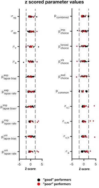
Next, we fit the model to individual subject data (as opposed to the aggregate) and obtained full posterior estimates over all model parameters for individual observers. We fit the model jointly to unisensory and causal inference tasks, such that we can constrain the sensory parameters by the observed unisensory data (Figure 1). The causal inference model provided a good and comparable fit for both ASD and control subjects (Figure 4E) with the model explaining more than 80% of explainable variance in all but one subject (Figure 4E, blue dot). Figure 4—figure supplements 36 show individual data for two representative control (Figure 4—figure supplements 3 and 4) and two ASD subjects (Figure 4—figure supplements 5 and 6), while highlighting all the data that constrained the model fits (audio localization, visual localization at three reliabilities, forced fusion task at three reliabilities, as well as implicit and explicit causal inference). Overall, both groups were heterogeneous (Figure 4F and G). Nonetheless, in agreement with the aggregate data, individuals with ASD had a higher prior probability of common cause than control subjects (Figure 4F) during the implicit task (p=0.02), where pcommon can be estimated independently from pchoice. When estimating pcombined (i.e. the combination of pcommon and pchoice) for the explicit task (Figure 4G), the parameter estimates extracted from the individual fits suggested no difference between ASD and control subjects (p=0.26), although numerically the results are in line with the aggregate data, suggesting a lower pcombined in ASD than control (see inter-subject variability in Figure 4F and G). Importantly, the aggregate and single subject fits concord in suggesting an explicit compensatory mechanism in individuals with ASD, given that pcommon is higher in ASD than control (when this parameter can be estimated in isolation) and a measure corrupted by explicit choice biases (i.e. pcombined) is not. Individual subjects’ pcommon and pcombined as estimated by the model did not correlate with ASD symptomatology, as measured by the AQ and SCQ (all p>0.17). Exploration of the model parameters in the ‘poor performers’ did not suggest a systematic difference between these subjects and other vis-à-vis their causal inference parameters.

Last, we consider a set of alternative models that could in principle account for differences in behavior across the aggregate control and ASD cohorts. The first alternative (alternative A) was a forced fusion model where all parameters were fit to the ASD aggregate subject, but pcommon was fixed to a value of 1. Thus, under this account the ASD subject always combines the cues irrespective of the disparity between them. Alternative B was a no fusion model, the opposite to Alternative A, where now all parameters were fit to the ASD aggregate subject, but pcommon was fixed to a value of 2. Alternative C had a lapse rate but no lapse bias. Last, alternative D allowed only the choice parameters to vary between control and ASD, but no inference or sensory parameter. For the implicit task, lapse rate, bias, and pchoice were allowed to vary. For the explicit task since pchoice trades off with pcommon, only lapse rate and bias were allowed to vary.

We performed model comparison using AIC and Figure 4—figure supplement 7 shows this metric for the ASD aggregate subject relative to the causal inference model where we vary choice and inference parameters (i.e. the model used in Figure 4. Lower AIC indicates a better fit). Figure 4—figure supplement 8 and Figure 4—figure supplement 9 show the original (choice and inference) and alternative fits, respectively, to implicit and explicit spatial causal inference tasks. For the implicit task, varying sensory and choice parameters, as opposed to inference parameters, results in a worse quality fit. Interestingly, alternative A (forced fusion) is a considerably better model than alternative B (forced segregation). Together, this pattern of results suggests that choice and inference (and not choice and sensory) parameters distinguish between ASD and control subjects in the implicit causal inference task. Likewise, these results further corroborate the conclusion that ASD subjects favor an internal model where integration outweighs segregation (AIC alternative A<AIC alternative B), yet there is not a complete lack of causal inference in ASD, given that alternative A is inferior to the model where pcommon is less than 1. In other words, individuals with ASD do perform causal inference, but they give more weight to integration (vs. segregation) compared to neurotypical subjects. For the explicit task, the alternative models considered performed worse than allowing the choice and inference parameters to vary (main model used in Figure 4).

For completeness, we fit the causal inference model to data from the simultaneity judgment task (see Figure 4—figure supplement 10 and Supplementary file 5), given that this task constitutes a large portion of the literature on multisensory impairments in ASD (see e.g. Feldman et al., 2018). However, in this task, given its explicit nature, it is also not possible to dissociate pchoice and pcommon (as for the explicit spatial task), and even more vexingly, given that reliabilities were not manipulated (as is typical in the study of multisensory temporal acuity, see Nidiffer et al., 2016, for an exception), it is also difficult to dissociate the pchoice from lapse parameters with a reasonable amount of data. We also explore the impact of lapse rates and biases and their differences across ASD and control subjects in Figure 4—figure supplement 11.

Discussion

We presented individuals with ASD and neurotypical controls with audio-visual stimuli at different spatial or temporal disparities, and measured their unisensory spatial discrimination thresholds, their implicit ability to perform optimal cue combination, and their implicit and explicit tendency to deduce different causal structures across cue disparities. The results indicate no overall impairment in the ability to perform optimal multisensory cue integration (Ernst and Banks, 2002). These observations generalize a previous report (Zaidel et al., 2015) and suggest that across domains (visuo-vestibular in Zaidel et al., 2015 audio-visual here), optimal cue combination is intact in ASD. Instead, we found that even at large spatial disparities, individuals with ASD use information from one sensory modality in localizing another. That is, in contrast to neurotypical controls, individuals with ASD behaved as if they were more likely to infer that cues come from the same rather the different sources. This suggests that the well-established anomalies in multisensory behavior in ASD - e.g., biases (see Baum et al., 2015 and Wallace et al., 2020, for reviews) – may not be due to a dysfunctional process of multisensory integration per se, but one of impair causal inference.

The juxtaposition between an impaired ability for causal inference yet the presence of an intact ability for optimal cue combination may suggest a deficit in a specific kind of computation and point toward anomalies in particular kinds of neural motifs. Indeed, an additional algorithmic component in causal inference (Körding et al., 2007) relative to optimal cue combination models (Ernst and Banks, 2002) is the presence of non-linear operations such as marginalization. This operation corresponds to ‘summing out’ nuisance variables, allows for non-linearities, and may be neurally implemented via divisive normalization (see Beck et al., 2011 for detail on marginalization and the relationship between this operation and divisive normalization). In fact, while not all proposed neural network models of causal inference rely on divisive normalization (see Cuppini et al., 2017; Zhang et al., 2019 for networks performing causal inference without explicit marginalization), many do (e.g. Yamashita et al., 2013; Yu et al., 2016). Divisive normalization is a canonical neural motif (Carandini and Heeger, 2011), i.e., thought to operate throughout the brain, wherein neural activity from a given unit is normalized by the joint output of a normalization neural pool. Thus, the broad anomalies observed in ASD may be underpinned by an alteration in a canonical computation, i.e., causal inference, which in turn is dependent on a canonical neural motif, i.e., divisive normalization. Rosenberg et al., 2015, suggested that anomalies in divisive normalization – specifically a reduction in the amount of inhibition that occurs through divisive normalization – —can account for a host of perceptual anomalies in ASD, such as altered local vs. global processing (Happé and Frith, 2006), altered visuo-spatial suppression (Foss-Feig et al., 2013), and increased tunnel vision (Robertson et al., 2013). This suggestion – from altered divisive normalization, to altered marginalization, and in turn altered causal inference and multisensory behavior – is well aligned with known physiology in ASD and ASD animal models showing decrease GABAergic signaling (Lee et al., 2017; Chen et al., 2020), the comorbidity between ASD and seizure activity (Jeste and Tuchman, 2015), and the hypothesis that ASD is rooted in an increased excitation-to-inhibition ratio (i.e. E/I imbalance; Rubenstein and Merzenich, 2003).

A second major empirical finding is that individuals with ASD seem to explicitly report common cause less frequently than neurotypical controls. Here we demonstrate a reduced tendency to explicitly report common cause during small cue disparities, across both spatial and temporal disparities (also see Figure 2—figure supplement 2E-G for corroborative evidence during a motion processing task). This has previously been observed within the temporal domain (Noel et al., 2018b; Noel et al., 2018a), yet frequently multisensory simultaneity judgments are normalized to peak at ‘1’ (e.g. Woynaroski et al., 2013; Dunham et al., 2020), obfuscating this effect. To the best of our knowledge, the reduced tendency to explicitly report common cause across spatial disparities in ASD has not been previously reported. Further, it is interesting to note that while ‘temporal binding windows’ were larger in ASD than control (see Feldman et al., 2018), ‘spatial binding windows’ were smaller in ASD relative to control subjects. This pattern of results highlights that when studying explicit ‘binding windows’, it may not be sufficient to index temporal or spatial domains independently, but there could potentially be a trade-off. More importantly, the reduced tendency to overtly report common cause across spatial and temporal domains in ASD (even when implicitly they seem to integrate more, and not less often) is indicative of a choice bias that may have emerged as a compensatory mechanism to their increased implicit tendency to bind information across sensory modalities. This speculation is supported by formal model fitting, where the prior probability of combination (p-common) was larger at the (aggregate) population level in the ASD than the control subjects in implicit tasks (where p-common may be independently estimated), yet a combined measure of p-common and a choice bias (these not being dissociable in explicit tasks such as spatial or temporal common cause reports) that was reduced (in the aggregate) or not significantly different (in the individual subject data) between ASD and control individuals. The presence of this putative compensatory mechanism is important to note, particularly when a significant fraction of the characterization of (multi)sensory processing in ASD relies on explicit tasks. Further, this finding, highlights the importance in characterizing both implicit and explicit perceptual mechanisms – particularly when framed under a strong theoretical foundation (Ernst and Banks, 2002; Körding et al., 2007) and using model-based analyses (e.g. Lawson et al., 2017; Lieder et al., 2019) – given that explicit reports may not faithfully reflect subjects’ percepts.

Last, it is also interesting to speculate on how an increased prior probability of integrating cues, and the presence of a compensatory mechanism, may relate to ASD symptomatology. Here we did not observe any reliable correlation between symptomatology and either psychophysical measures or model parameter estimates. However, it must be acknowledged that while the overall number of participants across all experiments was relatively large (91 subjects in total), our sample sizes within each experiment were moderate (~20 subjects per group and experiment), perhaps explaining the lack of any correlation. Regardless, it is well established that beyond (multi)sensory anomalies (Baum et al., 2015), individuals with ASD show inflexible and repetitive behaviors (Geurts et al., 2009) and demonstrate ‘stereotypy’, self-stimulatory behaviors thought to relieve sensory-driven anxiety (Cunningham and Schreibman, 2008). The finding that individuals with ASD do not change their worldview (i.e. from integration to segregation, even at large sensory disparities) may result in sensory anomalies and reflect the slow updating of expectations (Vishne et al., 2021). Thus, anomalies in causal inference may have the potential of explaining seemingly disparate phenotypes in ASD – anomalous perception and repetitive behaviors. Similarly, we may conjecture that stereotypy is a physical manifestation of a compensatory mechanism, such as the one uncovered here. Stereotypy could result from attempting to align incoming sensory evidence with the (inflexible) expectations of what that sensory input ought to be.

In conclusion, by leveraging a computational framework (optimal cue combination and causal inference; Ernst and Banks, 2002; Körding et al., 2007) and systematically measuring perception at each step (i.e. unisensory, forced cue integration, and causal inference) across a range of audio-visual multisensory behaviors, we can ascribe anomalies in multisensory behavior to the process of inferring the causal structure linking sensory observations to their hidden causes. Of course, this anomaly results in perceptual biases (see the current results and Baum et al., 2015 for an extensive review), but the point is that these biases are driven by a canonical computation that has gone awry. Further, given the known E/I imbalance in ASD (Rubenstein and Merzenich, 2003; Lee et al., 2017; Chen et al., 2020) and the fact that causal inference may require marginalization but optimal cue combination does not (Beck et al., 2011), we can speculatively suggest a bridge from neural instantiation to behavioral computation; E/I imbalance may disrupt divisive normalization (neural implementation), which leads to improper marginalization (algorithm) and thus altered causal inference (computation) and multisensory perception (biases in behavior) in ASD.

Materials and methods

Participants

A total of 91 adolescents (16.25±0.4 years; 20 females) took part (completely or partially) in a series of up to five behavioral experiments (four audio-visual and presented in the main text, in addition to a visual heading discrimination task presented in the Supplementary Materials). Forty-eight of these were neurotypical controls. Individuals in the control group (16.5±0.4 years; 13 females) had no diagnosis of ASD or any other developmental disorder or related medical diagnosis. These subjects were recruited by flyers posted throughout Houston. The other 43 participants (16.0±0.5 years; 7 females) were diagnosed as within ASD. The participants with ASD were recruited through several sources, including (1) the Simons Simplex Collection families, (2) flyers posted at Texas Children’s Hospital, (3) the Houston Autism Center, and (4) the clinical databases maintained by the Simons Foundation Autism Research Initiative (SFARI). All participants were screened at enrollment with SCQ (Rutter et al., 2003) and/or the AQ (Baron-Cohen et al., 2001) to afford (1) a measure of current ASD symptomatology and (2) rule out concerns for ASD in control subjects. There was no individual with ASD below the recommended SCQ cutoff, and only 2 (out of 47) control subjects above this cutoff (Surén et al., 2019). Similarly, there was almost no overlap in ASD and control AQ scores (with only 3 out of 47 control individuals having a higher AQ score than the lowest of the individuals with ASD). All individuals with ASD were above the AQ cutoffs recommended by Woodbury-Smith et al., 2005 and Lepage et al., 2009 (respectively, cutoff scores of 22 and 26), but not by Baron-Cohen et al., 2001 (cutoff score of 36). Inclusion in the ASD group required that subjects have (1) a confirmed diagnosis of ASD according to the DSM-5 (American Psychiatric Association, 2013) by part of a research-reliable clinical practitioner and (2) no history of seizure or other neurological disorders. A subset of the individuals with ASD were assessed by the Autism Diagnostic Observation Schedule (ADOS-2, Lord et al., 2012), and no difference was observed in the AQ, SCQ, or psychometric estimates between individuals with ASD with and without the ADOS assessment (all p>0.21). Similarly, the intelligence quotient (IQ) as estimated by the Wechsler Adult Intelligence Scale (WAIS) was available for a subset of the ASD participants (n=10, or 22% of the cohort), whose average score was 103±9 (S.E.M.), this being no different from the general population (which by definition has a mean of 100). All subjects had normal visual and auditory acuity, as characterized by parents’ and/or participants’ reports. For each of the five psychophysics experiments, we aimed at scheduling approximately 25–30 participants per group, in accord with sample sizes from previous similar reports (Dokka et al., 2019; Noel et al., 2018b). Data were not examined until after data collection was complete. The study was approved by the Institutional Review Board at the Baylor College of Medicine (protocol number H-29411) and written consent/assent was obtained.

Experimental materials and procedures

Experiment 1: Audio-visual spatial localization; maximum-likelihood estimation (implicit)

Thirty-one ASD (age = 15.2±0.4 years) and 34 control (16.1±0.4 years) subjects participated in this experiment. As expected, the SCQ (ASD = 17.1±0.75; control = 4.8±0.5; t-test: t63=–13.31, p<0.0001) and AQ scores (ASD = 31.2±1.7; control = 15.3±1.5; t41=–6.61, p<0.0001) of the ASD group were significantly greater than that of the control group.

Subjects performed a spatial localization task of auditory, visual, or combined audio-visual stimuli. A custom-built setup comprising of (1) an array of speakers and (2) a video projection system delivered the auditory and visual stimuli, respectively. Seven speakers (TB-F Series; W2-852SH) spaced 3° apart were mounted on a wooden frame along a horizontal line. A video projector (Dell 2,400 MP) displayed images onto a black projection screen (60 × 35°) that was mounted over the speaker array. This arrangement allowed presentation of the visual stimulus precisely at the location of the auditory stimulus, or at different locations on the screen. The auditory stimulus was a simple tone at 1200 Hz. The visual stimulus was a white circular patch. Reliability of the visual stimulus was manipulated by varying the size of the visual patch such that reliability inversely varied with the patch size (Alais and Burr, 2004). Three levels of visual reliability were tested: high (higher reliability of visual vs. auditory localization), medium (similar reliabilities of visual and auditory localization), and low (poorer reliability of visual vs. auditory localization). For high and low visual reliabilities, the patch diameter was fixed for all participants at 5 and 30°, respectively. For medium reliability, the patch diameter ranged from 15 to 25° across subjects. In all conditions (audio-only, visual-only, or combined audio-visual), the auditory and/or visual stimuli were presented for 50 ms (and synchronously in the case of combined stimuli). Stimuli were generated by custom MATLAB scripts employing the PsychToolBox (Kleiner et al., 2007; Noel et al., 2022).

Subjects were seated 1 m from the speaker-array with their chins supported on a chinrest and fixated a central cross. Subjects performed a single-interval, two-alternative-forced-choice spatial localization task. In each trial, they were presented with either an auditory, visual, or combined audio-visual stimulus (Figure 1A). They indicated if the auditory and/or visual stimulus were located to the left or right of straight forward by button-press. The spatial locations of the stimuli were varied in steps around straight forward. In single-cue auditory and combined conditions, the auditory stimulus was presented at one of the seven locations: 0,±3,±6, and ±9° (positive sign indicates that the stimulus was presented to the right of the participant). By contrast, the visual stimulus could be presented at any location on the screen. Specifically, in the single-cue visual condition, the visual stimulus was presented at ±20, ±10, ±5, ±2.5, ±1.25, ±0.65, ±0.32, and 0°. In the combined condition, auditory and visual stimuli were either presented at the same spatial location (Figure 1, top panel; Δ=0°) or at different locations separated by a spatial disparity Δ=±6° (Figure 1A, bottom panel; positive Δ indicates that the auditory stimulus was located to the right of the visual stimulus). For trials in which there was a spatial conflict, a mean stimulus location was defined. The auditory and visual stimuli were presented on either side of this mean stimulus location at an angular distance of Δ/2. For Δ=6°, the mean stimulus was located at –12, –9, –6, –3, 0, 3, and 6°. For Δ=–6°, the mean stimulus was located at –6, –3, 0, 3, 6, 9, and 12°. Each subject performed a total of 1680 trials (auditory condition = 7 stimulus locations × 15 repetitions; visual condition = 14 stimulus locations × 15 repetitions × 3 visual cue reliabilities; and combined auditory-visual condition = 7 stimulus locations × 3 reliabilities × 3 conflict angles × 15 repetitions). All conditions were interleaved.

For each subject, visual cue reliability, stimulus condition, and spatial disparity, psychometric functions were constructed by plotting the proportion of rightward responses as a function of stimulus location. These data were fit with a cumulative Gaussian function using psignifit, a MATLAB package that implements the maximum-likelihood method (Wichmann and Hill, 2001). The psychometric function yields two parameters that characterize participants’ localization performance: bias and threshold. Bias (μ) is the stimulus value at which responses are equally split between rightward and leftward. A bias close to 0° indicates highly accurate localization. The threshold is given by the SD (σ) of the fitted cumulative Gaussian function. The smaller the threshold, the greater the precision of spatial localization. The bias and threshold values estimated from these psychometric functions were used to test the predictions of optimal cue integration. The psychometric fitting could not estimate auditory thresholds for six ASD subjects, whose report did not vary as a function of auditory stimuli location. These subjects were not included in the remaining analyses reported in the main text.

Based on unisensory localization, we may derive predictions for the combined case, given optimal cue combination by maximum-likelihood estimation (Ernst and Banks, 2002; Hillis et al., 2002; Alais and Burr, 2004; Kersten et al., 2004). First, assuming optimal cue combination, the threshold in the combined auditory-visual condition (σcom) should be equal to:

σcom=σa2σv2σa2+σv2 (1)

with σa and σv being the thresholds in the unisensory auditory and visual localization, respectively. Second, the weight assigned to the visual cue in combined audio-visual stimuli (see Ernst and Banks, 2002 and Alais and Burr, 2004, for detail) should vary with its reliability. Specifically, as visual cue reliability decreases, the visual weight will also decrease. The visual weight, wv, is predicted to be:

Wv=1σv21σv2+1σa2 (2)

and in turn the auditory cue weight (wa) is computed as 1 − wv.

Experiment 2: Audio spatial localization with disparate visual cues; causal inference (implicit)

Twenty-two ASD (age = 17.32±0.57 years) and 15 control (age = 16.86±0.55 years) subjects participated in this experiment. As expected, the SCQ (ASD = 16.42±1.12; control = 5.06±0.65; t-test: t35=7.84, p<0.0001) and AQ scores (ASD = 31.95±1.76; control = 13.76±1.61; t35=7.21, p<0.0001) of the ASD group were significantly greater than that of the control group.

The task and stimuli employed here were identical to the audio-visual localization experiment described above, except that a larger range of spatial disparities were employed. The disparity between cues (∆) could take one of nine values: 0, ±3, ±6, ±12, and ±24°. Each ∆ was presented 8 times at each of the 7 speaker locations, and at each visual cue reliability, resulting in a total of 1512 trials (9 spatial disparities × 7 speaker locations × 3 reliabilities × 8 repetitions). Subjects indicated if the auditory stimulus was located to the right or left of straight ahead. Subjects were informed that the flash and beep could appear at different physical locations. All conditions were interleaved, and subjects were required to take breaks and rest after each block.

For each subject, audio-visual disparity (∆), and visual cue reliability, psychometric functions were constructed by plotting the proportion of rightward responses as a function of the true auditory stimulus location. As for the audio-visual localization task described above, data were fitted with a cumulative Gaussian function. An auditory bias close to 0° indicates that the subject was able to discount the distracting influence of the visual cues and accurately localize the audio beep. Data from one ASD subject was excluded from this analysis as the subject was unable to perform the task even when auditory and visual stimuli were co-localized (∆=0°). In eight ASD subjects, psychometric functions could not fit into the data even at the highest disparity (∆ = ±24°) during high reliability, as subjects’ estimates were ‘captured’ by the visual cues. The remaining data from these subjects were included in the analyses.

As an initial quantification of localization estimates, and putative differences in audio-visual biases between the groups, a third-order regression model of the form: y = a0 + a1∆ + a22 + a3American Psychiatric Association, 2013 was fitted to the auditory bias as a function of ∆ and visual cue reliability. Coefficient a1 represents how sensitive the bias is to changes in ∆ - larger a1 indicates a greater change in the bias for a given change in ∆. Coefficient a2 indicates if the dependence of bias on ∆ is uniform for positive and negative ∆ values. Importantly, coefficient a3 generally represents how the bias changes at large ∆ values – negative a3 indicates a saturation or a decrease in the bias at large ∆. If subjects perform causal inference (Körding et al., 2007), we expect a saturation or even a return to no bias at large ∆. Furthermore, partial R2 values associated with a1, a2, and a3 describe the contribution of each term in explaining the total variance. ASD and control subjects’ data was well-explained by the third-order regression model (ASD: R2=0.93±0.04; control: R2=0.88±0.03). A mixed-effects ANOVA with group, ∆, and visual cue reliability as factors compared the bias, threshold, and parameters of the regression model for the ASD and control groups.

Experiment 3: Audio-visual common source reports under spatial disparities (Explicit)

Twenty-three23 ASD (age = 16.14±0.51 years) and 24 control (age = 17.10±0.42 years) subjects participated in this experiment. Six other ASD subjects were screened for this experiment, but showed poor auditory localization (c.f. Experiment 1). The SCQ (ASD = 16.91±0.83; control = 5.04±0.47; t-test: t57=11.46, p<0.0001) and AQ scores (ASD = 30.77±1.60; control = 15.18±1.60; t41=6.42, p<0.0001) of the ASD group were significantly greater than that of the control group.

The auditory and visual stimuli presented in this task were identical to those employed in Experiment 2. Each ∆ was presented 7 times, at each of seven speaker locations, and at each visual cue reliability, resulting in a total of 1323 trials (9 spatial disparities × 7 speaker locations × 3 reliabilities × 7 repetitions). Subjects indicated via button-press if the auditory and visual cues originated from a common source or from different sources. The exact instructions were to “press the ‘same source’ key if auditory and visual signals come from the same source, and press the ‘different sources’ key if auditory and visual signals come from different sources.” All conditions were interleaved, and subjects were required to take breaks and rest after each block. Before the start of the main experiment, subjects participated in a practice block to familiarize themselves with the stimuli and response buttons. The response buttons (one for ‘same source’ and the other for ‘different sources’ were the left and right buttons of a standard computer mouse. Reports from eight ASD subjects did not vary with ∆, and thus their data was excluded from the main analyses).

For each subject, audio-visual disparity (∆), and visual cue reliability, the proportion of common source reports was calculated. A mixed-effects ANOVA with group as the between-subjects factor, along with ∆ and visual cue reliability as within-subjects factors compared the proportion of common source reports in 26 control and 25 ASD subjects.

Further, to quantify putative differences in how ASD and control subjects inferred the causal relationship between auditory and visual stimuli, Gaussian functions were fit to the proportion of common source reports as a function of ∆ (e.g. Rohe and Noppeney, 2015). These fits yielded three parameters of interest: (1) amplitude (tendency to report common cause when maximal), (2) mean (spatial disparity at which auditory and visual cues are most likely considered to originate from a common cause), and (3) width (spatial disparity range over which subjects are likely to report common cause).

Experiment 4: Audio-visual common source reports under temporal disparities (Explicit)

Twenty-one ASD (age = 15.94±0.56 years) and 19 control (age = 16.3±0.47 years) subjects participated in this task. As expected, ASD subjects had significantly higher SCQ (ASD: SCQ = 18.31±1; control: SCQ = 4.92±0.73; t-test: t32=–9.41, p<0.0001) and AQ (ASD: AQ = 32.76±1.58; control: AQ = 14.58±1.15; t-test: t32=7.43, p<0.0001) scores than the control subjects. Subjects viewed a flash and heard an audio beep (same stimuli as in Experiments 1, 2, and 3) presented centrally either at the same time or at different asynchronies. Twenty-three different temporal disparities (∆) were presented: 0, ±10, ±20, ±50, ±80, ±100, ±150, ±200, ±250, ±300, ±500, and ±700 ms (positive ∆s indicate that flash led the auditory stimulus). Subjects indicated if the flash and beep were synchronous (exact instruction: ‘appeared at the same time’) or asynchronous (‘appeared at different times’) via button press on a standard computer mouse. Each ∆ was presented 25 times in random order.

Proportion of synchronous reports at each ∆ was calculated. A Gaussian function was fit to the proportion of synchronous reports as a function of ∆ (ASD: R2=0.86±0.05; control: R2=0.94±0.01). The Gaussian fits yielded three parameters that characterized subjects’ performance: (1) amplitude (representing the maximum proportion of synchronous reports), (2) mean (representing the ∆ at which subjects maximally perceived the flash and beep to be synchronous), and (3) width (representing the range of ∆ within which subjects were likely to perceive the auditory and visual stimuli to co-occur in time).

A mixed-effects ANOVA with group as the between-subjects factor, and temporal disparity (∆) as a within-subjects factor compared the proportion of synchronous reports. Similarly, independent-samples t-tests compared the parameters of the Gaussian fits between the groups.

Experiment 5: Visual heading discrimination during concurrent object motion

Fourteen ASD and 17 control subjects (ASD: 15.71±0.5 years; control: 16.3±0.6 years) participated in this task. The ASD group had significantly higher SCQ (ASD: 16.71±1.36; control: SCQ = 7.35±1.12; p<0.0001) and AQ scores (ASD: AQ = 33.78±2.20; control = 11.79±2.35, p<0.0001) than the control group. Details of the apparatus and experimental stimuli have been previously described (Dokka et al., 2019).

In brief, subjects viewed lateral movement of a multipart spherical object while presented with a 3D cloud of dots mimicking forward translation (Figure 2—figure supplement 2A). The multipart object moved rightward or leftward within a fronto-parallel plane at five peak speeds: 0.07, 0.13, 0.8, 2.67, and 5.33 m/s. Implied self-motion consisted of a single interval, 1 s in duration, during which the motion stimulus followed a smooth Gaussian velocity profile (displacement = 13 cm; peak velocity = 0.26 m/s). Heading was varied in discrete steps around straight forward (0°), using the following set of values: 0, ±5, ±10, ±15, ±20, ±25, and ±45° (positive value indicates rightward heading). In one session, subjects indicated if they perceived the object to be stationary or moving in the world. In another session, subjects indicated if their perceived heading was to the right or left of straight ahead. In each session there were a total of 130 distinct stimulus conditions (2 object motion directions × 5 object motion speeds × 13 headings) and each condition was presented 7 times. All stimulus conditions were interleaved in each block of trials.

Heading discrimination performance was quantified by fitting psychometric curves for each object motion direction and speed (Dokka et al., 2019). These fits yielded parameters that characterize the accuracy and precision of heading perception: bias and threshold. For statistical analyses, the bias measured with leftward object motion was multiplied by –1, such that expected biases were all positive (Dokka et al., 2019). To quantify the differences in the heading bias between groups, a third-order regression model of the form: y = b0 + b1X + b2X2 + b3X3, where X is the sign consistent logarithm of object motion speed was fitted to the heading bias. We compared the linear (b1), quadratic (b2), and cubic (b3) coefficients along with their corresponding partial R2 values between groups, similar to the analyses performed on the auditory bias in the audio-visual localization tasks.

Causal Inference Modeling

We modeled subject responses using a causal inference model (Figure 4A) where the observer has to infer whether two sensory cues (auditory and visual) come from the same or separate causes(s), and use this information to either integrate or not information from these cues. In each trial, we assume that the subject’s observations of the auditory and visual location (denoted Xa and Xv) are the experimenter defined veridical values (denoted by ϵa and ϵv) corrupted by sensory noise with variances σa2 and σv2 ,

pXaϵa=N(Xa;ϵa,σa2) (3)
pXvϵv=N(Xv;ϵv,σv2) (4)

where N(x;μ,σ2) denotes the normal probability density function with mean μ and variance σ2 . We assume that subjects have a good estimate of their sensory uncertainties (over lifelong learning) and hence the subject’s estimated likelihoods become,

l(Sa)p(Xa|Sa)= N(Xa;Sa,σa2) (5)
l(Sv)p(Xv|Sv)= N(Xv;Sv,σv2) (6)

where Sa and Sv denote the inferred location of auditory and visual stimuli. The subject’s joint prior over the cue locations is parameterized as a product of three terms which reflect:

(a) fnaturalSa,Sv : the subject’s natural prior over the unisensory cue locations. For example, subjects may have a prior that sensory cue locations are more likely to occur closer to midline as compared to peripheral locations. We model this component of the prior as normal distributions where the mean and variance are unknown parameters fitted to the data.

fnaturalSa,Sv=NSa;μa,σap2NSv;μv,σvp2 (7)

(b) fCISa,Sv|C : the influence that the inferred cause (C) has on the knowledge of cue locations. In our causal inference model Sa is inferred as being equal to Sv if C=1 and independent if C=2.

fCI(Sa,Sv|C)={δ(saSv)ifC=11ifC=2 (8)

(c) ftaskSa|D : the relationship between the inferred trial category (D) and the cue locations.

Implicit task

In the implicit discrimination task, where the trial category corresponds to the side of the auditory cue location relative to the midline, Sa is positive if Dimp = 1 and negative if Dimp =-1.

 ftask(Sa,Sv|Dimp )={H(Sa)ifDimp=1H(Sa)ifDimp=1 (9)

where H(x) is the Heaviside function (H(x)=1 if x>0 and 0 otherwise).

The product of Equations 7–9, defines the probability over cue locations conditioned on C and Dimp in the implicit task as

pimplicitSa,Sv|C,DimpfnaturalSa,SvfCISa,Sv|CftaskSa,Sv|Dimp (10)

which can be succinctly written as

pimplicitSa,Sv|Dimp,CNSa;μa,σap2NSv;μv,σvp2C-1+(2-C)δSa-SvHDimpSa (11)

We parameterize the observer’s priors over Dimp and C as Bernoulli distributions with means pchoice and pcommon.

pimplicit(Dimp=1)=Ber(Dimp;pchoiceimplicit) (12)
p(C=1)=Ber(C;pcommon) (13)

The posterior probability of the subject inferring the auditory cue to come from the right can be obtained by marginalizing over the observer’s belief whether the auditory and visual cue come from a single or from separate causes

pimplicit(Dimp=1|Xa,Xv)=c1,2pimplicitDimp=1Xa,Xv,C=cp(C=c|Xa,Xv) (14)

We assume the subject makes their response by choosing the response that has the highest posterior probability. If Rimplicit is the subject response (1 for right and –1 for left), then

Rimplicit=argmaxd{-1,1}pimplicit(Dimp=d|Xa,Xv) (15)

Explicit task

We model the explicit task by assuming that the decision maker computes the belief over the trial category Dexp using the inferred belief over C, but not exactly equating both (graphical model in Figure 4A). This extends earlier approaches (Körding et al., 2007) which equate trial category Dexp with C, and additionally allows us to model task specific beliefs about the trial category. As we will show later, such a difference in beliefs between Dexp and C is mathematically equivalent to the subject making their decision by comparing their belief over C to a criterion different from 0.5.

The subject’s knowledge about the relationship between the trial category and the inferred variable C is parameterized as αtask , as given by Equation 16 and Equation 17

p(C=1|D=1)=Ber[C;pcommon+αtask1-pcommon] (16)
p(C=1|D=2)=Ber[C;pcommon-αtaskpcommon] (17)

For αtask=0 there is no relationship between trial category D and C (e.g. before learning the task), and thus the prior over C reduces to pcommon. On the other extreme, αtask=1 corresponds to complete task-learning, where C and Dexp are identical.

The prior probability of the subject’s belief over Dexp in the explicit task is parameterized as a Bernoulli distribution with mean pchoice as given in Equation 18

pexplicit(D=1)=Ber(D;pchoiceexplicit) (18)

We modeled subject’s belief about the sensory cue locations as the product of two terms: fnaturalSa,Sv and fCISa,Sv|C (Equation 7 and Equation 8)

pexplicit(Sa,Sv|C)  fnatural(Sa,Sv) fCI(Sa,Sv|C)
pexplicit(Sa,Sv|C){ fnatural(Sa,Sv)δ(SaSv),ifC=1fnatural(Sa,Sv),ifC=2 (19)

with appropriate normalization constants obtained by integrating over all Saand Sv , we get

pexplicit(Sa,Sv|C)={  N(Sa;μa,σap2)N(Sv;μv,σvp2)N(μa;μv,σap2+σvp2)δ(SaSv)ifC=1N(Sa;μa,σap2)N(Sv;μv,σvp2) ifC=2 (20)

Our model makes choice Rexplicit = 1 if

 pexplicit(D=1|Xa ,Xv)> pexplicit(D=2|Xa ,Xv) (21)

which by Bayes rule reduces to,

pexplicit(Xa ,Xv|D=1)pchoiceexplicit>    pexplicit(Xa ,Xv|D=2)(1-pchoiceexplicit) (22)

where the likelihood over observations is evaluated by marginalizing across inferred sensory locations using the sensory likelihoods (Equation 5 and Equation 6), i.e.,

pexplicitXa,Xv|C=c=pXa,Xv|Sa,SvpexplicitSa,Sv|C=cdSadSv (23)

We can marginalize out C in Equation 22 to get

pchoiceexplicit pexplicit(Xa,Xv|C=1)[pcommon+αtask(1pcommon)]+pchoiceexplicitpexplicit(Xa,Xv|C=2)[1pcommonαtask(1pcommon)]>(1pchoiceexplicit) pexplicit(Xa,Xv|C=1)[pcommonαtask(pcommon)]+(1pchoiceexplicit)pexplicit(Xa,Xv|C=2)[1pcommon+αtask(pcommon)] (24)

By combining terms, Equation 24 can be simplified as

 pexplicit(Xa,Xv|C=1)pcombined> pexplicit(Xa,Xv|C=2)(1-pcombined) (25)

where pcombined is a function of pcommon , pchoiceexplicit and αtask as given in Equation 26 which cannot be individually constrained.

pcombined=max(0,min(1,pcommon(2pchoiceexplicit1)+αtask[pcommon(1pchoiceexplicit+pchoiceexplicit(1pcommon))](2pcommon1)(2pchoiceexplicit1)+2αtask[pcommon(1pchoiceexplicit)+pchoiceexplicit(1pcommon)])) (26)

We now show that a decision rule as given in Equation 26 is equivalent to a subject making their decision by comparing their inferred posterior pexplicitC=1|Xa,Xv to a criterion t, i.e., Rexplicit =1 if

pexplicit(C=1|Xa,Xv)>t (27)

Or equivalently

pexplicit(C=1|Xa,Xv)(1t)>pexplicit(C=2|Xa,Xv)t (28)

which can be expanded using Bayes rule as given in Equation 29

pexplicit(Xa,Xv|C=1)(1t)pcommon>pexplicit(Xa,Xv|C=2)(t)(1pcommon) (29)

Comparing Equation 29 to Equation 25, we can relate terms to get

pcombined=(1-t)pcommon1-tpcommon +(t)(1-pcommon) (30)

where the criterion t is a function of pcommon, pchoiceexplicit and αtask .

We provide further model derivation and fitting details in Supplementary Materials, Supplementary file 3, Supplementary file 4. We can also similarly derive the causal inference model for the simultaneity judgement by modeling the temporal percepts as Bayesian inference and replacing the spatial disparities with temporal disparities. Further details are provided in the Supplementary Materials, (Supplementary file 5).

Last, as a contrast to the causal inference model (and variants thereof, alternatives A–D presented in the main text), for explicit tasks we also fit a functional form, specified by a Gaussian (mean and SD as free parameters) plus an additive bias (Figure 3—figure supplement 3). We fit this model to the spatial common cause reports (Figure 3A) of control subject. Then, we vary the additive bias, b (see Figure 3—figure supplement 3), in attempting to account for the ASD data relative to the control. Both the fit to the control data, and to the ASD data relative to the control, were better accounted for by the causal inference model (which additionally is a principled one), than the functional form.

Acknowledgements

We thank Jing Lin and Jian Chen for programming the experimental stimulus. This work was supported by NIH U19NS118246 (to RH and DEA), and by the Simons Foundation, SFARI Grant 396,921 and Grant 542949-SCGB (to DEA).

Funding Statement

The funders had no role in study design, data collection and interpretation, or the decision to submit the work for publication.

Contributor Information

Dora E Angelaki, Email: da93@nyu.edu.

Xiang Yu, Peking University, China.

Barbara G Shinn-Cunningham, Carnegie Mellon University, United States.

Funding Information

This paper was supported by the following grants:

  • National Institutes of Health NIH U19NS118246 to Dora E Angelaki, Ralf M Haefner.

  • Simons Foundation Autism Research Initiative 396921 to Dora E Angelaki.

Additional information

Competing interests

No competing interests declared.

No competing interests declared.

Author contributions

Conceptualization, Data curation, Formal analysis, Investigation, Methodology, Visualization, Writing - original draft, Writing – review and editing.

Conceptualization, Data curation, Formal analysis, Investigation, Methodology, Software, Visualization, Writing – review and editing.

Conceptualization, Data curation, Investigation, Methodology.

Conceptualization, Funding acquisition, Investigation, Methodology, Project administration, Resources, Supervision, Writing – review and editing.

Conceptualization, Funding acquisition, Project administration, Supervision, Writing – review and editing.

Ethics

Human subjects: The study was approved by the Institutional Review Board at the Baylor College of Medicine (protocol number H-29411) and written consent/assent was obtained.

Additional files

Supplementary file 1. Control participants.

The table indexes each control participant by a unit ID, and indicates in which experiment did each participant take part in. Green indicates that the participant took part in the given experiment, while red indicates that they did not. Experiment 1 is the unisensory discrimination task and audio-visual cue combination that does not require causal inference (i.e. imperceptible disparities). Experiment 2 is the audio-visual implicit causal inference experiment. Experiment 3 is the explicit causal inference experiment with spatial disparities. Experiment 4 is the explicit causal inference experiment with temporal disparities. Experiment 5 is the visual heading discrimination task during concurrent object-motion.

elife-71866-supp1.docx (47.8KB, docx)
Supplementary file 2. ASD participants.

The table indexes each ASD participant by a unit ID, and indicates in which experiment did each participant take part in. Green indicates that the participant took part in the given experiment, while red indicates that they did not. An orange box indicates that the participant took part in the experiment, but their data was excluded in presentation of the empirical results (but not the modeling of individual subjects, as indicated in the main text). Experiment 1 is the unisensory discrimination task and audio-visual cue combination that does not require causal inference (i.e. imperceptible disparities). Experiment 2 is the audio-visual implicit causal inference experiment. Experiment 3 is the explicit causal inference experiment with spatial disparities. Experiment 4 is the explicit causal inference experiment with temporal disparities. Experiment 5 is the visual heading discrimination task during concurrent object-motion.

elife-71866-supp2.docx (48.1KB, docx)
Supplementary file 3. Priors distributions over model parameters.
elife-71866-supp3.docx (29.5KB, docx)
Supplementary file 4. Causal inference model inference and fitting details.
elife-71866-supp4.docx (31.3KB, docx)
Supplementary file 5. Causal inference modeling for simultaneity judgments.
elife-71866-supp5.docx (30.2KB, docx)
Transparent reporting form

Data availability

Data and code are available at https://osf.io/6xbzt.

The following dataset was generated:

Noel S, Dokka HA. 2022. ASD Causal Inference. Open Science Framework. 6xbzt

References

  1. Acerbi L, Dokka K, Angelaki DE, Ma WJ. Bayesian comparison of explicit and implicit causal inference strategies in multisensory heading perception. PLOS Computational Biology. 2018;14:e1006110. doi: 10.1371/journal.pcbi.1006110. [DOI] [PMC free article] [PubMed] [Google Scholar]
  2. Alais D, Burr D. The ventriloquist effect results from near-optimal bimodal integration. Current Biology. 2004;14:257–262. doi: 10.1016/j.cub.2004.01.029. [DOI] [PubMed] [Google Scholar]
  3. American Psychiatric Association . Diagnostic and Statistical Manual of Mental Disorders. Washington, DC): American Psychiatric Publishing; 2013. [DOI] [Google Scholar]
  4. Baron-Cohen S, Wheelwright S, Skinner R, Martin J, Clubley E. The autism-spectrum quotient (AQ): evidence from Asperger syndrome/high-functioning autism, males and females, scientists and mathematicians. Journal of Autism and Developmental Disorders. 2001;31:5–17. doi: 10.1023/a:1005653411471. [DOI] [PubMed] [Google Scholar]
  5. Baum SH, Stevenson RA, Wallace MT. Behavioral, perceptual, and neural alterations in sensory and multisensory function in autism spectrum disorder. Progress in Neurobiology. 2015;134:140–160. doi: 10.1016/j.pneurobio.2015.09.007. [DOI] [PMC free article] [PubMed] [Google Scholar]
  6. Beck JM, Latham PE, Pouget A. Marginalization in neural circuits with divisive normalization. The Journal of Neuroscience. 2011;31:15310–15319. doi: 10.1523/JNEUROSCI.1706-11.2011. [DOI] [PMC free article] [PubMed] [Google Scholar]
  7. Cao Y, Summerfield C, Park H, Giordano BL, Kayser C. Causal Inference in the Multisensory Brain. Neuron. 2019;102:1076–1087. doi: 10.1016/j.neuron.2019.03.043. [DOI] [PubMed] [Google Scholar]
  8. Carandini M, Heeger DJ. Normalization as a canonical neural computation. Nature Reviews. Neuroscience. 2011;13:51–62. doi: 10.1038/nrn3136. [DOI] [PMC free article] [PubMed] [Google Scholar]
  9. Chen Q, Deister CA, Gao X, Guo B, Lynn-Jones T, Chen N, Wells MF, Liu R, Goard MJ, Dimidschstein J, Feng S, Shi Y, Liao W, Lu Z, Fishell G, Moore CI, Feng G. Dysfunction of cortical GABAergic neurons leads to sensory hyper-reactivity in a Shank3 mouse model of ASD. Nature Neuroscience. 2020;23:520–532. doi: 10.1038/s41593-020-0598-6. [DOI] [PMC free article] [PubMed] [Google Scholar]
  10. Cunningham AB, Schreibman L. Stereotypy in Autism: The Importance of Function. Research in Autism Spectrum Disorders. 2008;2:469–479. doi: 10.1016/j.rasd.2007.09.006. [DOI] [PMC free article] [PubMed] [Google Scholar]
  11. Cuppini C, Shams L, Magosso E, Ursino MA. A biologically inspired neurocomputational model for audiovisual integration and causal inference. The European Journal of Neuroscience. 2017;46:2481–2498. doi: 10.1111/ejn.13725. [DOI] [PubMed] [Google Scholar]
  12. de Winkel KN, Katliar M, Diers D, Bülthoff HH. Causal Inference in the Perception of Verticality. Scientific Reports. 2018;8:5483. doi: 10.1038/s41598-018-23838-w. [DOI] [PMC free article] [PubMed] [Google Scholar]
  13. Dokka K, DeAngelis GC, Angelaki DE. Multisensory Integration of Visual and Vestibular Signals Improves Heading Discrimination in the Presence of a Moving Object. The Journal of Neuroscience. 2015;35:13599–13607. doi: 10.1523/JNEUROSCI.2267-15.2015. [DOI] [PMC free article] [PubMed] [Google Scholar]
  14. Dokka K, Park H, Jansen M, DeAngelis GC, Angelaki DE. Causal inference accounts for heading perception in the presence of object motion. PNAS. 2019;116:9060–9065. doi: 10.1073/pnas.1820373116. [DOI] [PMC free article] [PubMed] [Google Scholar]
  15. Dunham K, Feldman JI, Liu Y, Cassidy M, Conrad JG, Santapuram P, Suzman E, Tu A, Butera I, Simon DM, Broderick N, Wallace MT, Lewkowicz D, Woynaroski TG. Stability of Variables Derived From Measures of Multisensory Function in Children With Autism Spectrum Disorder. American Journal on Intellectual and Developmental Disabilities. 2020;125:287–303. doi: 10.1352/1944-7558-125.4.287. [DOI] [PMC free article] [PubMed] [Google Scholar]
  16. Ernst MO, Banks MS. Humans integrate visual and haptic information in a statistically optimal fashion. Nature. 2002;415:429–433. doi: 10.1038/415429a. [DOI] [PubMed] [Google Scholar]
  17. Feldman JI, Dunham K, Cassidy M, Wallace MT, Liu Y, Woynaroski TG. Audiovisual multisensory integration in individuals with autism spectrum disorder: A systematic review and meta-analysis. Neuroscience and Biobehavioral Reviews. 2018;95:220–234. doi: 10.1016/j.neubiorev.2018.09.020. [DOI] [PMC free article] [PubMed] [Google Scholar]
  18. Foss-Feig JH, Tadin D, Schauder KB, Cascio CJ. A substantial and unexpected enhancement of motion perception in autism. The Journal of Neuroscience. 2013;33:8243–8249. doi: 10.1523/JNEUROSCI.1608-12.2013. [DOI] [PMC free article] [PubMed] [Google Scholar]
  19. Geurts HM, Corbett B, Solomon M. The paradox of cognitive flexibility in autism. Trends in Cognitive Sciences. 2009;13:74–82. doi: 10.1016/j.tics.2008.11.006. [DOI] [PMC free article] [PubMed] [Google Scholar]
  20. Haefner RM, Cumming BG. An improved estimator of Variance Explained in the presence of noise. Advances in neural information processing systems; 2008. [PMC free article] [PubMed] [Google Scholar]
  21. Happé F, Frith U. The weak coherence account: detail-focused cognitive style in autism spectrum disorders. Journal of Autism and Developmental Disorders. 2006;36:5–25. doi: 10.1007/s10803-005-0039-0. [DOI] [PubMed] [Google Scholar]
  22. Hillis JM, Ernst MO, Banks MS, Landy MS. Combining sensory information: mandatory fusion within, but not between, senses. Science (New York, N.Y.) 2002;298:1627–1630. doi: 10.1126/science.1075396. [DOI] [PubMed] [Google Scholar]
  23. Hospedales T, Vijayakumar S. Multisensory oddity detection as bayesian inference. PLOS ONE. 2009;4:e4205. doi: 10.1371/journal.pone.0004205. [DOI] [PMC free article] [PubMed] [Google Scholar]
  24. Jeste SS, Tuchman R. Autism Spectrum Disorder and Epilepsy: Two Sides of the Same Coin? Journal of Child Neurology. 2015;30:1963–1971. doi: 10.1177/0883073815601501. [DOI] [PMC free article] [PubMed] [Google Scholar]
  25. Kersten D, Mamassian P, Yuille A. Object perception as Bayesian inference. Annual Review of Psychology. 2004;55:271–304. doi: 10.1146/annurev.psych.55.090902.142005. [DOI] [PubMed] [Google Scholar]
  26. Kleiner M, Brainard D, Pelli D, Ingling A, Murray R, Broussard C. What’s new in psychtoolbox-3. Perception. 2007;36:1–16. [Google Scholar]
  27. Körding KP, Beierholm U, Ma WJ, Quartz S, Tenenbaum JB, Shams L. Causal inference in multisensory perception. PLOS ONE. 2007;2:e943. doi: 10.1371/journal.pone.0000943. [DOI] [PMC free article] [PubMed] [Google Scholar]
  28. Lawson RP, Rees G, Friston KJ. An aberrant precision account of autism. Frontiers in Human Neuroscience. 2014;8:302. doi: 10.3389/fnhum.2014.00302. [DOI] [PMC free article] [PubMed] [Google Scholar]
  29. Lawson RP, Mathys C, Rees G. Adults with autism overestimate the volatility of the sensory environment. Nature Neuroscience. 2017;20:1293–1299. doi: 10.1038/nn.4615. [DOI] [PMC free article] [PubMed] [Google Scholar]
  30. Lee E, Lee J, Kim E. Excitation/Inhibition Imbalance in Animal Models of Autism Spectrum Disorders. Biological Psychiatry. 2017;81:838–847. doi: 10.1016/j.biopsych.2016.05.011. [DOI] [PubMed] [Google Scholar]
  31. Lepage JF, Lortie M, Taschereau-Dumouchel V, Théoret H. Validation of French-Canadian versions of the Empathy Quotient and Autism Spectrum Quotient. Canadian Journal of Behavioural Science / Revue Canadienne Des Sciences Du Comportement. 2009;41:272–276. doi: 10.1037/a0016248. [DOI] [Google Scholar]
  32. Lieder I, Adam V, Frenkel O, Jaffe-Dax S, Sahani M, Ahissar M. Perceptual bias reveals slow-updating in autism and fast-forgetting in dyslexia. Nature Neuroscience. 2019;22:256–264. doi: 10.1038/s41593-018-0308-9. [DOI] [PubMed] [Google Scholar]
  33. Lord C, Rutter M, DiLavore PC, Risi S, Gotham K, Bishop SL. Autism Diagnostic Observation Schedule. Torrance, CA: Western Psychological Services; 2012. [Google Scholar]
  34. Magnotti JF, Ma WJ, Beauchamp MS. Causal inference of asynchronous audiovisual speech. Frontiers in Psychology. 2013;4:798. doi: 10.3389/fpsyg.2013.00798. [DOI] [PMC free article] [PubMed] [Google Scholar]
  35. Nidiffer AR, Stevenson RA, Krueger Fister J, Barnett ZP, Wallace MT. Interactions between space and effectiveness in human multisensory performance. Neuropsychologia. 2016;88:83–91. doi: 10.1016/j.neuropsychologia.2016.01.031. [DOI] [PMC free article] [PubMed] [Google Scholar]
  36. Noel JP, Lytle M, Cascio C, Wallace MT. Disrupted integration of exteroceptive and interoceptive signaling in autism spectrum disorder. Autism Research. 2018a;11:194–205. doi: 10.1002/aur.1880. [DOI] [PMC free article] [PubMed] [Google Scholar]
  37. Noel JP, Stevenson RA, Wallace MT. Atypical audiovisual temporal function in autism and schizophrenia: similar phenotype, different cause. The European Journal of Neuroscience. 2018b;47:1230–1241. doi: 10.1111/ejn.13911. [DOI] [PMC free article] [PubMed] [Google Scholar]
  38. Noel JP, Lakshminarasimhan KJ, Park H, Angelaki DE. Increased variability but intact integration during visual navigation in Autism Spectrum Disorder. PNAS. 2020;117:11158–11166. doi: 10.1073/pnas.2000216117. [DOI] [PMC free article] [PubMed] [Google Scholar]
  39. Noel JP, Paredes R, Terrebonne E, Feldman JI, Woynaroski T, Cascio CJ, Seriès P, Wallace MT. Inflexible Updating of the Self-Other Divide During a Social Context in Autism: Psychophysical, Electrophysiological, and Neural Network Modeling Evidence. Biological Psychiatry. Cognitive Neuroscience and Neuroimaging. 2021a:00090–00092. doi: 10.1016/j.bpsc.2021.03.013. [DOI] [PMC free article] [PubMed] [Google Scholar]
  40. Noel JP, Zhang LQ, Stocker AA, Angelaki DE. Individuals with autism spectrum disorder have altered visual encoding capacity. PLOS Biology. 2021b;19:e3001215. doi: 10.1371/journal.pbio.3001215. [DOI] [PMC free article] [PubMed] [Google Scholar]
  41. Noel JP, Angelaki DE. Cognitive, Systems, and Computational Neurosciences of the Self in Motion. Annual Review of Psychology. 2022;73:103–129. doi: 10.1146/annurev-psych-021021-103038. [DOI] [PMC free article] [PubMed] [Google Scholar]
  42. Noel JP, Shivkumar SD, Haefner K. ASD Causal Inference. Open Science Framework. 2022 https://osf.io/6xbzt
  43. Odegaard B, Wozny DR, Shams L. Biases in Visual, Auditory, and Audiovisual Perception of Space. PLOS Computational Biology. 2015;11:e1004649. doi: 10.1371/journal.pcbi.1004649. [DOI] [PMC free article] [PubMed] [Google Scholar]
  44. Perdreau F, Cooke JRH, Koppen M, Medendorp WP. Causal inference for spatial constancy across whole body motion. Journal of Neurophysiology. 2019;121:269–284. doi: 10.1152/jn.00473.2018. [DOI] [PubMed] [Google Scholar]
  45. Robertson CE, Kravitz DJ, Freyberg J, Baron-Cohen S, Baker CI. Tunnel vision: sharper gradient of spatial attention in autism. The Journal of Neuroscience. 2013;33:6776–6781. doi: 10.1523/JNEUROSCI.5120-12.2013. [DOI] [PMC free article] [PubMed] [Google Scholar]
  46. Robertson CE, Baron-Cohen S. Sensory perception in autism. Nature Reviews. Neuroscience. 2017;18:671–684. doi: 10.1038/nrn.2017.112. [DOI] [PubMed] [Google Scholar]
  47. Rohe T, Noppeney U. Cortical hierarchies perform Bayesian causal inference in multisensory perception. PLOS Biology. 2015;13:e1002073. doi: 10.1371/journal.pbio.1002073. [DOI] [PMC free article] [PubMed] [Google Scholar]
  48. Rohe T, Noppeney U. Distinct Computational Principles Govern Multisensory Integration in Primary Sensory and Association Cortices. Current Biology. 2016;26:509–514. doi: 10.1016/j.cub.2015.12.056. [DOI] [PubMed] [Google Scholar]
  49. Rohe T, Ehlis AC, Noppeney U. The neural dynamics of hierarchical Bayesian causal inference in multisensory perception. Nature Communications. 2019;10:1907. doi: 10.1038/s41467-019-09664-2. [DOI] [PMC free article] [PubMed] [Google Scholar]
  50. Rosenberg A, Patterson JS, Angelaki DE. A computational perspective on autism. PNAS. 2015;112:9158–9165. doi: 10.1073/pnas.1510583112. [DOI] [PMC free article] [PubMed] [Google Scholar]
  51. Rubenstein JLR, Merzenich MM. Model of autism: increased ratio of excitation/inhibition in key neural systems. Genes, Brain, and Behavior. 2003;2:255–267. doi: 10.1034/j.1601-183x.2003.00037.x. [DOI] [PMC free article] [PubMed] [Google Scholar]
  52. Rutter M, Bailey A, Lord C. The Social Communication Questionnaire: Manual. Western Psychological Services; 2003. [Google Scholar]
  53. Sawai KI, Sato Y, Aihara K. Auditory time-interval perception as causal inference on sound sources. Frontiers in Psychology. 2012;3:524. doi: 10.3389/fpsyg.2012.00524. [DOI] [PMC free article] [PubMed] [Google Scholar]
  54. Series P. Computational Psychiatry. MIT Press; 2020. [Google Scholar]
  55. Smith E, Zhang S, Bennetto L. Temporal synchrony and audiovisual integration of speech and object stimuli in autism. Research in Autism Spectrum Disorders. 2017;39:11–19. doi: 10.1016/j.rasd.2017.04.001. [DOI] [PMC free article] [PubMed] [Google Scholar]
  56. Surén P, Saasen-Havdahl A, Bresnahan M, Hirtz D, Hornig M, Lord C, Reichborn-Kjennerud T, Schjølberg S, Øyen AS, Magnus P, Susser E, Lipkin WI, Stoltenberg C. Sensitivity and specificity of early screening for autism. BJPsych Open. 2019;5:e41. doi: 10.1192/bjo.2019.34. [DOI] [PMC free article] [PubMed] [Google Scholar]
  57. van den Berg R, Vogel M, Josic K, Ma WJ. Optimal inference of sameness. PNAS. 2012;109:3178–3183. doi: 10.1073/pnas.1108790109. [DOI] [PMC free article] [PubMed] [Google Scholar]
  58. Vishne G, Jacoby N, Malinovitch T, Epstein T, Frenkel O, Ahissar M. Slow update of internal representations impedes synchronization in autism. Nature Communications. 2021;12:5439. doi: 10.1038/s41467-021-25740-y. [DOI] [PMC free article] [PubMed] [Google Scholar]
  59. Wallace MT, Woynaroski TG, Stevenson RA. Multisensory Integration as a Window into Orderly and Disrupted Cognition and Communication. Annual Review of Psychology. 2020;71:193–219. doi: 10.1146/annurev-psych-010419-051112. [DOI] [PubMed] [Google Scholar]
  60. Wichmann FA, Hill NJ. The psychometric function: I. Fitting, sampling, and goodness of fit. Perception & Psychophysics. 2001;63:1293–1313. doi: 10.3758/bf03194544. [DOI] [PubMed] [Google Scholar]
  61. Woodbury-Smith MR, Robinson J, Wheelwright S, Baron-Cohen S. Screening adults for Asperger Syndrome using the AQ: a preliminary study of its diagnostic validity in clinical practice. Journal of Autism and Developmental Disorders. 2005;35:331–335. doi: 10.1007/s10803-005-3300-7. [DOI] [PubMed] [Google Scholar]
  62. Woynaroski TG, Kwakye LD, Foss-Feig JH, Stevenson RA, Stone WL, Wallace MT. Multisensory speech perception in children with autism spectrum disorders. Journal of Autism and Developmental Disorders. 2013;43:2891–2902. doi: 10.1007/s10803-013-1836-5. [DOI] [PMC free article] [PubMed] [Google Scholar]
  63. Yamashita I, Katahira K, Igarashi Y, Okanoya K, Okada M. Recurrent network for multisensory integration-identification of common sources of audiovisual stimuli. Frontiers in Computational Neuroscience. 2013;7:101. doi: 10.3389/fncom.2013.00101. [DOI] [PMC free article] [PubMed] [Google Scholar]
  64. Yu Z, Chen F, Dong J, Dai Q. Sampling-based causal inference in cue combination and its neural implementation. Neurocomputing. 2016;175:155–165. doi: 10.1016/j.neucom.2015.10.045. [DOI] [Google Scholar]
  65. Zaidel A, Goin-Kochel RP, Angelaki DE. Self-motion perception in autism is compromised by visual noise but integrated optimally across multiple senses. PNAS. 2015;112:6461–6466. doi: 10.1073/pnas.1506582112. [DOI] [PMC free article] [PubMed] [Google Scholar]
  66. Zhang W, Wu S, Doiron B, Lee TS. A Normative Theory for Causal Inference and Bayes Factor Computation in Neural Circuits. Advances in Neural Information Processing Systems. 2019;32:3804–3813. [Google Scholar]

Editor's evaluation

Xiang Yu 1

Autism spectrum disorder is characterized by social, communicative and sensory anomalies. This study uses behavioral psychophysics experiments and computational modelling to interrogate how individuals with autism combine sensory cues in multisensory tasks. The results showed that individuals with autism were more likely to integrate cues, but less likely to report doing so, thus raising interesting questions regarding how individuals with autism perceive the world.

Decision letter

Editor: Xiang Yu1
Reviewed by: Ulrik Beierholm2

In the interests of transparency, eLife publishes the most substantive revision requests and the accompanying author responses.

Decision letter after peer review:

Thank you for submitting your article "Aberrant causal inference and presence of a compensatory mechanism in Autism Spectrum Disorder" for consideration by eLife. Your article has been reviewed by 3 peer reviewers, and the evaluation has been overseen by a Reviewing Editor and Richard Ivry as the Senior Editor. The following individual involved in review of your submission has agreed to reveal their identity: Ulrik Beierholm (Reviewer #3).

The reviewers have discussed their reviews with one another, and the Reviewing Editor has drafted this to help you prepare a revised submission.

Essential revisions:

1) The experiments report interesting results regarding audio-visual integration for spatial discriminations in both typical individuals and individuals with ASD. However, the conceptual framing (including the model) is one of several potential accounts of these data, and should be framed as such. Alternative accounts need to be presented and seriously discussed, and not just as an extension of the Discussion. The abstract and other parts of the manuscript also need to be adjusted accordingly.

2) Related to point 1. Prominent aspects of the data, including higher overall bias in autism in Figure 2, are not captured in the model in Figure 4. The dissociation between explicit and implicit is not convincing, and the stress on group differences puts an emphasis on small effects. Please revise model and/or Discussion to address these concerns.

3) Model fitting is not described sufficiently. How were the sensory parameters fitted? It seems that more than 20 parameters were fitted (Supp. File 1) for the aggregate subject through the slice sampling, is that correct? Was this also done for individual subjects? What was done to ensure convergence? Was any model comparison done? Please include a list or figure showing the different steps of the model fitting.

4) The model may be over-specified with both a lapse rate and a lapse bias. Please test a simpler model without lapse bias or explain why that was not done.

5) In experiments 3 and 4 please detail the specific instructions given. Specifically, were participants asked to press a button if they thought both cues come from the same source, or if they thought that the 2 cues come from 2 sources? Since there was not a default option (an "I don't know option"), it's important to know the default – determined by the way the question was phrased.

6) The participants in each experiment were not clearly described. Please provide more details about the task completion of participants, such as how many completed all four tasks, etc. A table would be helpful. Specifically, what were the performance scores in Experiment 1 – of the sub-group of participants of Experiment 2 – the question of whether the psychometric plots did not differ between ASD and controls participating in this study is crucial for estimating whether they were expected to have different magnitudes of bias (as they actually did). The authors did not address the question of the overall bias magnitude, only the values at the large disparities.

7) Please specify the criteria for the ASD diagnosis, DSM-5 or DSM-4? Are they classic autism or Asperger or PDD-NOS subjects? Were the gold standard ADOS ADIR performed to confirm the diagnosis? If not, the authors should acknowledge this as a limitation in Discussion.

8) More detailed research participant description is required. SCQ and AQ were performed for all participants. Were there ASD individuals below the cut-off of these two scales? or any TD participants above the cut-off? This information should be stated. The authors should consider excluding the ASD individuals below the cut-offs and TD individuals above the cut-offs from data analysis. Please provide more details about how the TD participants were recruited. IQ was available for a subset of the ASD participants: How many of them have IQ scores? IQ was measured using what test? Was the IQ measured for the TD group?

9) Please report effect sizes, e.g. eta2 or Cohen's d.

Reviewer #1:

Using a series of cue combination tasks, the authors studied the causal inference of multisensory stimuli in people with ASD. The authors found the intact ability in optimal cue combination of participants with ASD but impairment in dissociating audio and visual stimuli when presented with wider spatial disparity. It suggested they persisted with a wrong integration model for causal inference. However, the individuals with ASD explicitly report the common cause of stimuli fewer than the controls. Through formal modeling, the authors found increased prior probability for the common cause in ASD. However, reporting the common cause in ASD is reduced in the explicit task, indicative of a compensatory mechanism via a choice bias.

In general, I think this study was well-designed and the results were interesting. The conclusions of this paper are mostly well supported by data. But I have a few questions that I would like to see the author’s address.

1. When comparing the temporal disparity task to the spatial task, the authors concluded that the overall reduced tendency to report common cause at any disparity and across spatial and temporal conflicts seemingly is the defining characteristic of ASD. However, in Figure 3D, it could tell that a higher proportion of common cause reporting in ASD when absolute temporal disparity became greater, which differed from the case of spatial task and from when the temporal disparity was narrower. Could the conclusion be too general? The authors should tone it down or give more discussion about the incongruence.

2. When fitting the model to individual subject data, the authors found comparable pcombined for the explicit task between ASD and control subjects. This seemed to be contrasted to the result of aggregate data and behavioral results. Did the difference come from the fitting procedure? Did the significant decreased in pcombined was because of the lack of consideration of subject heterogeneity? The authors could provide more explanation or discussion of it.

3. A related question is about the intuition behind the two steps of modeling fitting (i.e., to aggregate and individual data). What more could fitting models to aggregate or individual data provide to one another procedure? The authors should elaborate on it.

4. I would like to see the authors discuss more the interesting finding of a potential compensatory mechanism, particularly the meaning of it in terms of the possible relation to ASD symptoms. For example, how would the increased prior probability of common cause report and the compensatory choice bias contribute to the sensory abnormalities in ASD?

5. The participants in each experiment were not clearly introduced. The authors should provide more details about the task completion of participants, such as how many completed all four tasks, etc. And the data of how many participants who participated in both the implicit and explicit spatial task were included in modeling?

6. The authors could also conduct some correlational analyses between estimated model parameters and symptomatology measures, just as what they have done for psychometric features, to further investigate how autistic symptoms would affect the process of causal inference.

7. Since the data of the individuals with poor performance were also fitted (such as 8 of the individuals with ASD in Experiment 3), it is interesting to see if there is anything special or atypical in terms of their model parameters, even though their data were not included in behavioral analyses.

8. I suggest specifying the criteria for the ASD diagnosis, DSM-5? or DSM-4? or ICD-10? Are they classic autism or Asperger or PDD-NOS? Were the gold standard ADOS ADIR performed to confirm the diagnosis? If not, the authors should acknowledge this as the limitation in Discussion.

9. SCQ and AQ were performed to all participants. My question is: is there any ASD individuals below the cut-off of these two scales? or any TD participants above the cut-off. the authors should consider excluding the ASD individuals below the cut-offs and TD individuals above the cut-offs from the data analysis.

10. Please provide more details about how the TD participants were recruited?

11. IQ was available for a subset of the ASD participants: How many of them have IQ scores? Is there any particular reason that the other ASD participants did not have IQ scores? How the IQ was measured? using Wechesler or Raven's test? Was the IQ measured for the TD group?

12. The authors could provide direct comparisons of thresholds and visual weights between two groups in the result section of Experiment 1.

13. Errors bars in Figure 1E and 1H were not very obvious. The authors could consider using simpler markers, such as "+" (i.e., short lines) for simultaneously displaying horizontal and vertical error bars.

14. It should be "As for the case of auditory disparities, …" instead of " As for the case of spatial disparities, …" for the first sentence of the second paragraph after Figure 3.

Reviewer #2:

The paper consists of 4 interesting experiments examining multisensory processing in autism spectrum disorder. The first experiment shows that participants with ASD perform similar to controls in cross-model integration, a conceptual replication of earlier findings from this group. However, the subsequent experiments reveal some intriguing differences between the groups in terms of how they use explicit and implicit information in evaluating if auditory and visual information comes from a common source or distinct sources. The authors propose a model that aims to explain the seeming dissociation between explicit and implicit reports of the two groups. The strength of this work is that the experiments are very interesting and report interesting results regarding audio-visual integration for spatial discriminations in both typical individuals and people with ASD. The comparison between explicit and implicit reports is very interesting. In terms of weaknesses, the dissociation between explicit and implicit is not convincing, and the stress on group differences puts an emphasis on, at best, marginal effects, which the modelling does not explain. For example, an alternative account that is consistent with all the data presented is that there are individuals with ASD who are somewhat poorer auditory discriminators, resulting in the bias effects and broader disparities. These individuals would be less likely to commit to an explicit "single source" statement in line with their reduced auditory localization skills.

The dissociation between explicit and implicit is not convincing, and the stress on group differences puts an emphasis on, at best, marginal effects, which the modelling does not explain (the strongest linearity on ASD's curve in Figure 2 – is not captured in the modelling in Figure 4) For example, an alternative account that is consistent with all the data presented is that there are individuals with ASD who are somewhat poorer auditory discriminators and they impacted overall performance in Experiment 2, resulting in a larger bias effect, and also somewhat broader in disparities. These individuals would be less likely to commit to an explicit "single source" statement, which is quite committing, in line with their reduced auditory localization skills. The authors should at least address this alternative account, and present auditory discrimination curves of Experiment 2's participants.

The model does not account for the data point of individuals with autism being pulled by a reliable visual blob 24 degrees away, which was the main point in Figure 3.

Overall the authors ignore more prominent aspects of the data (e.g. higher overall bias in autism in Figure 2) for points they want to make (non linearity larger in autism than in controls).

Reliability – is a confusing term. The stimuli are reliably presented, but the information the perceivers derive regarding their position is less reliable when stimuli are small.

Figure 1f, g – I had difficulties understanding. I assume that the dashed lines should be to the right of the solid lines, which is the case for "high-reliability" blob, but why is it switched for the low reliability case? In both sample participants (f and g) and I wonder why the bias is larger (larger distance between dashed and matched solid plot, in both participants) for low versus intermediate size (reliability) blobs. If this is the actual result – it needs explanation.

Figure 2 – the main observation is that the bias in autism is larger. Perhaps this group difference stems from this group being somewhat poorer auditory spatial discriminators than their 15 age-matched controls in the experiment. If their auditory discrimination is poorer we would expect an overall larger bias, and perhaps also across a broader range of audio-visual disparities.

Importantly, this is probable account, since this is a smaller population than in Experiment 1 – and their discrimination thresholds are not addressed. Importantly – I could not figure out the overlap in participation across the various experiments. In experiment 1 matched performance was only obtained when 6 participants with ASD were excluded. In Experiment 3 (24 participants originally) – they also excluded a large subgroup, whose behavior was different. Here the group is initially small so variability across participants was not discussed.

The strongest point for the claim of too broad integration is the bottom left point – where high reliability blob has an effect that even increases when the visual blob is presented 24 degrees apart. This point is hard to reconcile (and is not reconciled by the model proposed in Figure 4 either). The authors should show that it is a reliable data point – perhaps by showing single subject data.

In experiments 3 and 4 the specific instructions are crucial – are participants asked to press a specific button if they are perceived as coming from the same source? Or press a button if they are perceived as coming from 2 separate sources. Here phrasing may have affected the decisions of individuals with autism. In order to dissociate between these 2 options it would have been nice to have a third option "don't know". If participants with autism tend to say to be less decisive they would tend to commit to a single source. This account may be explained by being somewhat implicitly poorer localizers.

If you have discrimination functions of the specific subgroups that took part in Experiments 2-3 (since they all participated in Experiment 1 – right?) – please show them or report discrimination skills for these subgroups, since this is the relevant control-ASD matching.

Re modelling and Figure 4 – It is difficult to follow the model – perhaps label the model parameters in the diagram of Figure 4a.

Reviewer #3:

In this paper Noel et al., use a combination of psychophysical experiment and computational modeling to examine the differences in behaviour between participant on the Autism Spectrum Disorder and control participants when dealing with multi-sensory stimuli (e.g. audio-visual). It is well known that ASD subjects tend to differ in how they combine such stimuli, and it has previously been suggested that this may be due to a difference in the tendency to perform causal inference.

The study indeed finds that while ASD participants had similar ability to combine cues when unambiguously from the same source, they differed in the tendency to combine them when unclear if necessary to combine. In contrast when asked to explicitly indicate whether stimuli originated from the same source (and therefore should be combined) they tended to under report.

While the experiments are in themselves very standard, the paper relies on computational modeling to differentiate the possible behavioural effects, using advanced Bayesian statistical methods.

These results confirm existing ideas, and build on our understanding of ASD, while still leaving many questions unanswered. The results should be of interest to anyone studying ASD as well as any other developmental disorders, and perception in general.

I enjoyed reading this paper, although the model fitting procedure especially was not clear to me. How were the sensory parameters fitted? By my count more than 20 parameters were fitted (Supp. File 1) for the aggregate subject through the slice sampling, is that correct? Was this also done for individual subjects? I would be nervous about fitting that many parameters for individual subject data. What was done to ensure convergence?

Was any model comparison done? Might be better to include a list or figure showing the different steps of the model fitting.

I also worry that the model is over specified with both a lapse rate and a lapse bias. From my understanding the lapse rate specifies when subjects (through lack of concentration or otherwise) fail to take trial stimuli into account and therefore go with their prior. In other studies this prior may be identical to the prior over spatial range, or may be a uniform discrete distribution over the bottoms available for response.

Maybe the variables are constrained in ways that I did not understand, but with just a binary response (Left/Right) the model can largely incorporate any bias to a large set of possible parameter values of lapse rate and bias. I.e. that the model is over specified. That would also explain the wide range of values for the fitted parameters in Figure 3.

I think this should really be investigated before the results can be trusted.

Looking at Figure 4E and F makes me hesitant about trusting the results.

Authors also acknowledge that the lapse bias and P combined are too closely entwined to really be well separated in the explicit temporal experiment. Maybe for that reason it would also be useful to test a simpler model without lapse bias?

I find it mildly confusing that D refers to a Left/Right response in the implicit task, and Common/Separate in the explicit task. Maybe better to use separate symbols? D is fine for 'decision' but in places in the text it is instead referred to as 'trial category' which is vague. I also don't really think D is needed in the generative model in Figure 4 as it is not really causing the subsequent variables C or Sa.

Does eLife not require the reporting of effect sizes (e.g. eta2 or Cohen's d)? It would be good to include these.

The plots in Figure 3 mostly look like shifts up for ASD relative to controls. The authors might want to fit a model with a positive bias, i.e.

a*N(mu,sd2)+b

may fit better (could do model comparison) and just show difference in b. This is just a suggestion though, but it may be cleaner for their argument.

In the Discussion, while divisive normalisation is one way to achieve the marginalisation needed for Bayesian causal inference, there are other ways to achieve it (Cuppino et al., 2017, Yamashita 2013, Yu et al., 2016, Zhang et al., 2019). It would be good to acknowledge this.

Eq 5 and 6, 38 are misleading. Likelihood is a function of Sa/Sv, so would be better to write as l(Sa)=N(Xa;Sa,Sv)

Eq 9: is D either 1 or 2? Or 1 or -1?

Detail: maybe use different symbols for lapse rate and lapse bias? I find λ and odell confusing. How about Plapse for the lapse rate to emphasise that it is a probability? Pcommon is already a fitted variable that is also a probability of a Bernoulli distribution.

Page 5 (pages of the pdf):

“ …ASD did not show impairments in integrating perceptually congruent auditory and visual stimuli.”

– “ …ASD did not show impairments in integrating perceptually congruent (and near-congruent) auditory and visual stimuli.”

In experiment 2 there was a six degree discrepancy, so near-congruent seems appropriate.

Typos:

“We perform the integral in Eq. S5 for the implicit task by”: should this be Eq. 35?

References:

Cuppini, C., Shams, L., Magosso, E. and Ursino, M. A biologically inspired neurocomputational model for audiovisual integration and causal inference. Eur. J. Neurosci. 46, 2481-2498 (2017).

Yamashita, I., Katahira, K., Igarashi, Y., Okanoya, K. and Okada, M. Recurrent network for multisensory integration-identification of common sources of audiovisual stimuli. Front. Comput. Neurosci. 7, (2013).

Yu, Z., Chen, F., Dong, J. and Dai, Q. Sampling-based causal inference in cue combination and its neural implementation. Neurocomputing 175, 155-165 (2016).

Zhang, W., Wu, S., Doiron, B. and Lee, T. S. A Normative Theory for Causal Inference and Bayes Factor Computation in Neural Circuits. Adv. Neural Inf. Process. Syst. 32, 3804-3813 (2019).

[Editors’ note: further revisions were suggested prior to acceptance, as described below.]

Thank you for resubmitting your work entitled “Aberrant causal inference and presence of a compensatory mechanism in Autism Spectrum Disorder” for further consideration by eLife. Your revised article has been evaluated by Barbara Shinn-Cunningham (Senior Editor) and a Reviewing Editor.

All reviewers agree that the manuscript has improved significantly during revision, but there are some remaining issues to be addressed, as noted below and described in detail in the individual reviews:

1. More detailed description of how statistical analysis was carried out, including clarifications/modifications as suggested by reviewer 1.

2. Rebalancing interpretation of the experimental and odelling results, as suggested by reviewer 2.

Reviewer #1:

The authors have addressed my recommendations and questions in much detail. Their changes have improved the quality of the manuscript as a result, illuminating the perceptual causal inference in ASD across different contexts. However, I believe there still are a couple of points that the authors can address to make the description of the results and the methods even clearer for publication.

1. Figure legends/captions of Figures 3 and 4 in the main texts lack detailed descriptions of the elements in the figures. For example, for Figures 3 and 4, what do those error bars represent? Standard errors or confidence intervals? In Figure 4B, are solid lines the model predictions and hollow points the observations? I believe this essential information would help readers better understand the figures.

2. The data points in Figure 2A-B and Figure 3A-C are slightly different from those in Figure 4B-C. For example, in Figure 2B, the audio bias of 24 deg disparity is weaker than that of 12 deg disparity for the high visual reliability condition (dark brown lines and points); however, in Figure 4B left panel, the audio bias of 24 deg disparity is even larger than that of 12 deg disparity. I assume that the data points depicted in Figure 4B-C are the aggregate data for modelling, in which the data of some participants were not included? I notice that the authors have included which participants were included in the single-subject modelling, but was the aggregate data the same as what was used for plotting Figures 2 and 3? I find it a bit confusing at first sight, perhaps the author could check it again and/or mention the related information in the caption or the main text?

3. From lines 451-453 of merged files (Instead, differences between […] relative to control observers.), did the author imply that the model where pcommon was freely estimated from the data was better, compared with the model where pcommon was fixed (I guess it’s the model in Figure 4 – supplement 2)? In other words, did the authors have two different models and conduct a model comparison here? If so, I think it’s better to provide model comparison results. The question also applies to the texts from lines 460-461. Also, what is DAIC? Is it the difference of AIC between the full model (that allows pcommon) and the restricted model (that fixes pcommon to a constant)? The authors should describe it somewhere in the main text.

4. The authors should be more specific about the tests they used to compare model parameters between groups and those correlational analyses. What type of tests did the authors use, parametric (i.e., Welch t-test, Pearson correlation) or non-parametric (i.e., Mann-Whitney, Spearman correlation, or permutation methods)? Particularly for the comparison of pcombined (Figure 4G), would the result be different when a non-parametric test was used if the test used in the current revision was parametric? I suggest the authors take more robust approaches given that the distributions of the model parameters seemed not quite Gaussian.

5. What is α and ν in Equation 5 and 6, please define them in the text. Also, it would be better if the authors give a short introduction to the meaning of lapse rate, lapse bias, etc., when mentioning them for the first time. Given that many readers are not very familiar with computational modelling, they may not intuitively understand what these parameters represent.

6. The D in DAIC from line 462 is in another font.

7. I apologize in advance if it’s my mistake but I failed to find Supplementary Text 1 mentioned in lines 430, 451, and 459. Where could I find it?

Reviewer #2:

The authors have adequately addressed my comments.

The strong aspects of the results are better clarified, and the overlap between participants across experiments is also clear. Further, the authors do not make claims that are not directly supported experimentally.

The limitation of a somewhat small (<20) number of participants per group in important experiments is still a drawback, given participants’ variability, particularly in the ASD group. Yet, I believe that the main results hold.

The strongest aspects of the study are the direct results, rather than the modelling:

Experiment 1: audio-visual integration is intact in ASD 2. Yet multisensory behavior is atypical (in the current experimental protocol) – ASD participants tend to favor source integration, as manifested by their cross-modal bias in localization even when visual and auditory signal are separable from a sensory perspective. Though both groups tend to over integrate, this is more salient and tend to span a broader distance in ASD. 3. Explicit reports have an opposite tendency – individuals with ASD were less likely to report a common cause for the two stimuli. Given the adequate direct measures of ASD cue integration with a small audio-visual distance (performance in Experiment 1) these results suggest a specific atypicality in cause attribution.

I also find the difference between spatial and temporal integration very interesting. Temporal and spatial groups differences in explicit attribution of a common source merits some additional discussion.

Personally, I think the contribution of the modelling part to the study is overstated in the paper, but I agree that is a personal perspective and need not be imposed on the authors.

Reviewer #3:

The authors have done a very good job including new alternative models, and improving the Description of the modelling (modelling my main points of scepticism). I am happy to recommend the paper for publication.

eLife. 2022 May 17;11:e71866. doi: 10.7554/eLife.71866.sa2

Author response


Essential revisions:

1) The experiments report interesting results regarding audio-visual integration for spatial discriminations in both typical individuals and individuals with ASD. However, the conceptual framing (including the model) is one of several potential accounts of these data, and should be framed as such. Alternative accounts need to be presented and seriously discussed, and not just as an extension of the Discussion. The abstract and other parts of the manuscript also need to be adjusted accordingly.

We thank the reviewers for their suggestion and agree that presenting alternative accounts will strengthen the manuscript. We have done this both empirically and via additional modelling.

Empirically, we check whether visual and/or auditory localization performance is equal across the control and ASD cohorts participating in the causal inference task. We now report the auditory and visual discrimination bias and thresholds for these participants (Figure 2 – supplement figure 1). The results show no difference between controls and individuals with ASD, suggesting that a potential baseline difference in sensory processing between these groups does not explain their differing behavior during causal inference.

In additional modelling, we have now included the following potential accounts (see Figure 4 – supplement figure 7, 8, and 9):

A. Forced fusion (all parameters are free to vary, except for C, which is fixed to 1).

B. Forced segregation (all parameters are free to vary, except for C, which is fixed to 2).

C. Uniform lapse bias (Lapse rate, pcommon, pchoice are free to vary with a uniform lapse bias – unbiased model).

D. D1. Implicit task: Lapse rate, lapse bias, and pchoice are free to vary, others are not.

D2. Explicit task: Since pchoice trades off against pcommon for the explicit task, alternative D2 is similar to D1 (above), but only lapse rate and bias are free to vary.

In alternatives A and B, we fit the model to the ASD aggregate data. In models C and D, we first fit to the control aggregate subject, and then vary the specific parameters noted to fit to the ASD aggregate subject relative to the control. We report AICs for the ASD aggregate subject.

For the implicit task (most cleanly indexing pcommon), all alternative accounts perform worse than the model included in the main text (where lapse rate, lapse bias, pcommon and pchoice are free to vary from control to ASD aggregate subjects; see Figure 4 – supplement figure 7). This suggests that how individuals with ASD infer causal relations, and not their sensory uncertainty, is the most parsimonious factor differentiating between ASD and control (having excluded alternatives A and B that allow for different sensory uncertainties while fixing the causal inference parameter). Further, the fact that alternative A (forced fusion) does better than alternative B (forced segregation) again suggests that individuals with ASD tend to overweight integration relative to segregation. The fact that the model in the main text performs better than Alternative A suggests that individuals with ASD do not always integrate, they do perform causal inference, but are biased toward integration over segregation compared to controls.

In response to this comment, we have modified the text to include the unisensory performance for participants in Experiment 2 (P6, “To confirm […] and across all reliabilities), as well as the alternative models (P10-11, “Lastly, we consider a set of alternative models […]” vary (main model used in Figure 4)). We have also included new supplementary figures:

– Figure 2 – supplement figure 1. Visual and auditory localization performance of participants in Experiment 2 (audio-visual implicit causal inference).

– Figure 4 – supplement figure 7. Goodness-of-fit of alternative models for the implicit and explicit spatial causal inference task.

– Figure 4 – supplement figure 8. Illustration of the alternative models fits to implicit causal inference model data.

– Figure 4 – supplement figure 9. Illustration of the alternative models fits to explicit causal inference model data.

Lastly, we have included tables specifying which participants took part in the different experiments (in order to examine unisensory performance only of those subjects performing the causal inference task):

– Supplement File 1. Control participants.

– Supplement File 2. ASD participants.

2) Related to point 1. Prominent aspects of the data, including higher overall bias in autism in Figure 2, are not captured in the model in Figure 4. The dissociation between explicit and implicit is not convincing, and the stress on group differences puts an emphasis on small effects. Please revise model and/or Discussion to address these concerns.

The reviewers are correct in pointing out that the model illustrated in Figure 4 (aggregate data) does not fully account for all aspects of the data. However, we must note that we present the aggregate fits to highlight what parameters could or could not in principle explain global differences between the ASD and control cohort. In other words, while the aggregate subjects highlight the common or differing patterns across the two cohorts (ASD and control), even if all subjects used a causal inference strategy, the aggregate subject need not have a pattern completely consistent with the predictions of a causal inference model. On the other hand, the individual subject fits are very good (Figure 4E), with all but one subject showing an explainable variance explained above 80%. To further illustrate the quality of these fits – particularly considering that all experiments are fit jointly! – in this revision we have included supplementary figures showing example control (Figure 4 – supplement figure 3, 4) and ASD (Figure 4 – supplement figure 5, 6) subjects. Again, we must reiterate that we do not fit individual models to account for a particular experiment, but instead attempt to account for a subject’s behavior as a whole, across experiments and sensory modalities.

In the original submission, to highlight global differences between the ASD and control cohorts in a principled manner, we fixed all the sensory parameters (given the results in Experiment 1 showing no unisensory difference across groups) and only allowed for flexibility in the choice and inference parameters. Our new analyses presented in Figure 2 – supplement figure 1, Figure 4 – supplement figure 7 (see above), and Figure 3 – supplement figure 1 (unisensory performance for subjects taking part in Experiment 3), all concord in supporting the fact that there is no difference in sensory performance between the ASD and control cohorts. Nonetheless, we have now also tested this explicitly by testing an alternative model where the sensory uncertainty and choice parameters were allowed to vary from control to ASD (Figure 4 – supplement figure 2) but pcommon was fixed to the value of the aggregate control (similar to Alternatives A and B above, but where C is fixed to the aggregate control value, as opposed to C=1 or C=2). This model performed worse than that in the main text, where pcommon and choice parameters were allowed to vary. This indicates that a difference in pcommon explains better the difference between ASD and control subjects as compared to differences in sensory uncertainty. We also point out that for the individual subjects, sensory uncertainties were fit along with the inference parameters, and we found a significant difference in pcommon for ASD and control subjects. We found no difference in the estimated sensory uncertainty.

Similarly (and going beyond prior studies) here we fit data from all visual reliabilities jointly, which considerably constrains the model. In Figure 4 – supplement figure 12 (implicit task) and Figure 4 – supplement figure 13 (explicit task) we now demonstrate that either allowing all parameters to vary freely (Panel A), fitting all visual reliabilities separately (Panel B), or doing both of these together (Panel C), would have resulted in better aggregate fits. Even though these alternative models do not concord with our data showing no difference in sensory performance between ASD subjects and controls, these models yield similar results to those reported in the main text, with pcommon being numerically higher in ASD vs. control subjects, further demonstrating that this (our central) result is highly robust.

Lastly, the reviewers suggest that the group effect is small. To ascertain whether a difference in implicit causal inference between ASD and controls is a robust and replicable effect, and to probe its generalizability beyond audio-visual localization, we have now conducted a conceptual replication and extension. We follow the protocols from Dokka et al., 2019 (PNAS), where observers see a pattern of optic flow indicating translation slightly leftward or rightward. Further, they see an independent object, moving at different speeds. Subjects are asked to report their heading (leftward or rightward), and whether the object was stationary or moving. This is a causal inference task, given that if the object is perceived as stationary (hence part of the optic flow), it’s movement on our retinas ought to influence heading perception, but not if the object is perceived to be moving. In Figure 2 – supplement figure 2 (new addition to the revision) we demonstrate that just as for the audio-visual case, control subjects are biased by the independently moving object when this one has a slow speed in the world (similar to the optic flow), but not a fast speed. On the other hand, individuals with ASD seem to readily integrate the independent object into their own heading discrimination, even at large disparities. This is an important conceptual replication of the audio-visual experiment, and thus, even if the effect may be small, it appears to be a reliable one, and a domain general effect.

In response to this comment, we have modified the text to describe the methods (P17, section “Experiment 5: Visual heading discrimination during concurrent object motion”) and results (P6, “Lastly, to further bolster […] segregation (Figure S2C, D).”) of the replication and extension to the implicit causal inference experiment. We have also further described the goodness-of-fit of the aggregate and individual subject fits (P10, “The causal inference model […] as well as implicit and explicit causal inference”).

The following supplementary figures (and appropriate text and figure captions) have been included to (i) illustrate the additional implicit causal inference experiment (Figure 2 – supplement figures 1 and 2), and (ii) explicitly show single subject fits (Figure 4 – supplement figures 3-6) as well as alternative fits (e.g., fitting all visual reliabilities separately, or fitting sensory uncertainty but not p-common, Figure 4 – supplement figures 2, 12, and 13):

– Figure 2 – supplement figure 2. Heading discrimination during concurrent implied self-motion and object motion (Dokka et al., 2019).

– Figure 3 – supplement figure 1. Visual and auditory localization performance of participants in Experiment 3 (audio-visual explicit causal inference).

– Figure 4 – supplement figure 2. Fit to aggregate data for the implicit causal inference task, allowing sensory uncertainty and choice parameters to vary but fixing the inference parameter pcommon.

– Figure 4 – supplement figure 3. Data and fit for a single, representative control subject

– Figure 4 – supplement figure 4. Data and fit for another single, representative control subject

– Figure 4 – supplement figure 5. Data and fit for a single, representative ASD subject

– Figure 4 – supplement figure 6. Data and fit for another single, representative ASD subject.

– Figure 4 – supplement figure 12. Fit to aggregate data for the implicit causal inference task, given that all parameters are free to vary (A), the different visual reliabilities are fit separately (B) or both of the above (C).

– Figure 4 – supplement figure 13. Fit to aggregate data for the odellin causal inference task, given that all parameters are free to vary (A), the different visual reliabilities are fit separately (B) or both of the above (C).

3) Model fitting is not described sufficiently. How were the sensory parameters fitted? It seems that more than 20 parameters were fitted (Supp. File 1) for the aggregate subject through the slice sampling, is that correct? Was this also done for individual subjects? What was done to ensure convergence? Was any model comparison done? Please include a list or figure showing the different steps of the model fitting.

We thank the reviewers for their question and apologize this was not clearer in the original submission.

Indeed, each subject had 20 parameters characterizing their responses, yet they were constrained by a large dataset, including four types of tasks (unisensory discrimination, multisensory discrimination, implicit causal inference, and explicit causal inference) and three different visual reliabilities. Further, the prior over the parameters reduces the effective degrees of freedom, such that several parameters have their values tied together (unless constrained to be a specific value based on the empirical data) – equivalent to hierarchical modelling. We have chosen this approach to allow for differences in parameters (e.g., lapse) across experiments that were conducted on different days, but a-priori assuming they are the same. Similarly, when we fit the model to a single (or a subset of) experiment(s), then the parameters specific to the experiment are inferred to be the same as the prior (maximum of prior for the MAP estimate and the prior distribution for the inferred posterior). Therefore, for the aggregate control subject we are effectively fitting 12 parameters for the implicit task and 11 parameters for the explicit task (subset relevant for each task). Moreover, since the model was fit to multiple reliabilities, the prior parameters that were shared across reliabilities were constrained by data from all three reliabilities. For the ASD aggregate subject, either only the choice parameters were varied, or the choice and pcommon were varied relative to the aggregate control.

We followed a similar procedure for the individual subject fits, but now utilizing their respective empirical data to constrain the parameters. The prior over the parameters is shared as is typical for hierarchical odelling. For the individual subjects, we infer full posteriors over all parameters using slice sampling. The convergence of the sampling was checked by the potential scale factor reduction R^ across chains. Therefore, when we look at the marginal distribution over pcommon or pcombined, we marginalize out the other parameters as given by Equation R1. This implicitly performs model averaging by considering different models parameterized by different values of the parameters weighed by their posterior.

p(θinterest|data)=p(θinterest|data,θother)p(θother|data)(Equation R1)

In response to the reviewers’ comment, we have summarized the model fitting procedure, both in text (P9-10, “To bridge […] the two experimental groups”) and as a flowchart in the supplementary materials (Figure 4 – supplement figure 1).

4) The model may be over-specified with both a lapse rate and a lapse bias. Please test a simpler model without lapse bias or explain why that was not done.

Allowing for a lapse rate and a lapse bias separately is mathematically equivalent to allowing for two different lapse parameters, each corresponding to a different choice – as is commonly done (e.g., Schütt et al., 2016). We define a prior over lapse bias which is weakly informative, peaking at 0.5. This is the traditional assumption about lapse bias (i.e., unbiased). Therefore, under such a definition, we infer a lapse bias that is different from the commonly assumed 0.5 value if and only if the data has support under such a model. However, as per the reviewers’ suggestion, we have now also tested an alternative (Alternative C in response to Question #1) where only the lapse rate and pcommon were allowed to vary. As alluded to above, this model had a higher AIC (poorer fit) as compared to also allowing for a lapse bias. For individual subjects, the pcommon recovered when considering this simpler model was also higher for ASD as compared to control subjects (p=0.008). Similarly, the pcombined was not different between the two populations. Thus, the results are consistent with the model allowing for a lapse bias, as presented in the main paper.

5) In experiments 3 and 4 please detail the specific instructions given. Specifically, were participants asked to press a button if they thought both cues come from the same source, or if they thought that the 2 cues come from 2 sources? Since there was not a default option (an "I don't know option"), it's important to know the default – determined by the way the question was phrased.

We thank the reviewers for this question and apologize that we had not provided enough information regarding the instructions. The short answer is that participants were asked to press one button for a given report (e.g., “common cause”) and another for the opposite report (e.g., “separate cause”). Thus, there was no imbalance in the effort required to give one response vs. the other – i.e., there was no default. This important information has now been included in the text (P16, “The exact instructions were […] a standard computer mouse”. And, P17, “Subjects indicated […] standard computer mouse”).

6) The participants in each experiment were not clearly described. Please provide more details about the task completion of participants, such as how many completed all four tasks, etc. A table would be helpful. Specifically, what were the performance scores in Experiment 1 – of the sub-group of participants of Experiment 2 – the question of whether the psychometric plots did not differ between ASD and controls participating in this study is crucial for estimating whether they were expected to have different magnitudes of bias (as they actually did). The authors did not address the question of the overall bias magnitude, only the values at the large disparities.

We have now included in the manuscript Supplement File 1 and Supplement File 2, listing exactly which participants took part in the different experiments (see above). We have also made explicit in the text the inclusion criteria for data in the modeling effort. As suggested by the reviewers, most (but not all, ~80%) participants in Experiments 2 and 3 also took part in Experiment 1, and thus we could detail their visual and auditory localization performance. As we show in Figure 2- supplement figure 1 and Figure 3 – supplement figure 1 (novel additions to the text) there was no difference between the control and ASD sub-groups that participated in Experiments 2 and 3 in terms of their unisensory localization performance. Thus, we can attribute their anomalies in implicit and explicit audio-visual causal inference to the latter computation.

We also wish to highlight the considerable effort it represents to recruit ~40 ASD and ~40 control adolescents to participate in a series of up to 5 experiments (4 in the original manuscript and an additional one added in revisions). Each task took about 60 to 90 minutes to complete and were completed on different days to avoid fatigue. Given that most participants could not transport themselves, on many occasions appointments were missed, rescheduled, and canceled given the caretakers availability. Still, we collected a total of 220 sessions worth of psychophysical data, which represents a significant contribution (particularly when these tasks are informed by a computational approach as is the case here).

7) Please specify the criteria for the ASD diagnosis, DSM-5 or DSM-4? Are they classic autism or Asperger or PDD-NOS subjects? Were the gold standard ADOS ADIR performed to confirm the diagnosis? If not, the authors should acknowledge this as a limitation in Discussion.

The individuals with ASD were diagnosed according to the DSM-5 (which does not distinguish anymore between classic autism and Aspergers). A subset of these subjects (depending on how they were recruited) also counted with an ADOS assessment. There was no statistical difference in AQ, SCQ, or any of the psychometric estimates between ASD individuals with and without ADOS assessment (all p > 0.21). This suggests that all individuals categorized as within the autism spectrum were appropriately diagnosed. We have amended the text to include this information (P14, “Inclusion in the ASD group […] assessment (all p > 0.21).)

8) More detailed research participant description is required. SCQ and AQ were performed for all participants. Were there ASD individuals below the cut-off of these two scales? or any TD participants above the cut-off? This information should be stated. The authors should consider excluding the ASD individuals below the cut-offs and TD individuals above the cut-offs from data analysis. Please provide more details about how the TD participants were recruited. IQ was available for a subset of the ASD participants: How many of them have IQ scores? IQ was measured using what test? Was the IQ measured for the TD group?

There was no individual with ASD below the recommended SCQ cutoff. There were 2 (out of 47, or 4%, i.e., below the false positive rate) control subjects above the recommended cutoff for the SCQ. The AQ is more complicated, given that different cutoffs have been proposed. Most importantly, there were only 3 control subjects with a higher AQ score than the lowest AQ score among all individuals with ASD. All individuals with ASD had AQ scores above the cutoff proposed by 2 out of 3 published recommendations. The text has been modified to include this information (P14, “There was no individual with ASD below […] by Baron-Cohen et al., 2001, cutoff score of 36”).

Excluding the control subjects above the SCQ cutoff / overlapping in AQ score with the ASD subject with the lowest score, did not change the statistical interpretation of any of the reported effects.

The IQ was not measured for the TD group, but we know the mean of the population (by construction) is 100. Thus, we can assume the mean of the TD group was about this value. We only had access to a subset of IQ scores in the ASD cohort (n = 10), because certain clinical providers assessed this metric, while others did not (and thus whether we had an IQ score or not depended on how the subject was recruited). IQ was measured by the Wechsler Adult Intelligence Scale (which is also appropriate for adolescents). The text has been amended to include this information (P14, “Similarly, the Intelligence Quotient […] mean of 100”).

9) Please report effect sizes, e.g. eta2 or Cohen's d.

Thank you for the suggestion. We now report them throughout the manuscript.

Reviewer #1:

Using a series of cue combination tasks, the authors studied the causal inference of multisensory stimuli in people with ASD. The authors found the intact ability in optimal cue combination of participants with ASD but impairment in dissociating audio and visual stimuli when presented with wider spatial disparity. It suggested they persisted with a wrong integration model for causal inference. However, the individuals with ASD explicitly report the common cause of stimuli fewer than the controls. Through formal modeling, the authors found increased prior probability for the common cause in ASD. However, reporting the common cause in ASD is reduced in the explicit task, indicative of a compensatory mechanism via a choice bias.

In general, I think this study was well-designed and the results were interesting. The conclusions of this paper are mostly well supported by data. But I have a few questions that I would like to see the author’s address.

1. When comparing the temporal disparity task to the spatial task, the authors concluded that the overall reduced tendency to report common cause at any disparity and across spatial and temporal conflicts seemingly is the defining characteristic of ASD. However, in Figure 3D, it could tell that a higher proportion of common cause reporting in ASD when absolute temporal disparity became greater, which differed from the case of spatial task and from when the temporal disparity was narrower. Could the conclusion be too general? The authors should tone it down or give more discussion about the incongruence.

We thank the reviewer for their suggestion. We have now eliminated all reference to the difference in amplitude being the “defining characteristic”. Instead, we weigh equally the fact that individuals with ASD have both a shallower amplitude at small temporal disparities, and a larger width in the Gaussian describing reports of common cause as a function of temporal disparity. The result section has been modified to reflect this change (P9, “As for the case of spatial disparities […] “binding windows”).

In the Discussion section we also eliminated reference to the difference in amplitude as being the “defining characteristic” differentiating ASD from control individuals. We do, however, discuss this finding given that it was present in both the spatial and temporal task (also the visual heading discrimination task included during these revisions) and it is less often acknowledged (relative to the difference in “temporal binding windows”, e.g., Feldman et al., 2018).

Importantly, our modeling strongly implicates the difference in pcommon as the key difference between ASD subjects and controls in the context of a causal inference task.

2. When fitting the model to individual subject data, the authors found comparable pcombined for the explicit task between ASD and control subjects. This seemed to be contrasted to the result of aggregate data and behavioral results. Did the difference come from the fitting procedure? Did the significant decreased in pcombined was because of the lack of consideration of subject heterogeneity? The authors could provide more explanation or discussion of it.

The fitting procedure is slightly different, given that in one case we are using aggregate data, while in the other we are fitting to the individual subjects and thus we can leverage knowledge of the subject-specific sensory parameters.

The aggregate subject fitting was performed to highlight what parameters could or could not explain the global differences between ASD and control subjects. To do so, we considered a restricted model class where we assumed matched sensory parameters between ASD and control subjects (based on the findings from Experiment 1, and now Figure 2 – supplement figure 1 and Figure 2 – supplement figure 1). This approach increased the explanatory power of the model by restricting ourselves to a specific model class. This is similar to a bias-variance trade-off whereby introducing a bias (assumption of model family), we can reduce the variance in parameter estimates. Another reason for the aggregate subject having a higher explanatory power is that the aggregate subject has more data (scaled by number of subjects) which also increases the certainty of the estimates. This modelling approach, on the other hand, cannot capture subject heterogeneity, as pointed out by the reviewer. Hence, we also perform the single subject fits.

The individual subject data was fit across experiments and on a per subject level. We allowed for a more flexible model class given that we could estimate also sensory uncertainty parameters. This approach results in better fits (see response to questions above) but increases the heterogeneity in individual parameter estimates.

Overall, we do not think the results are contradictory. First, because slightly different approaches to model fitting were taken. These different approaches maximize the information we may gain, with the aggregate fits attempting to explain global differences between groups and the single subject fits trying to account for individual difference in the observed behavior. Second, there is no conceptual contradiction while there being strong differences in statistical power. In fact, the results are numerically congruent (between aggregate and individual subject). The individual subject data does not differ significantly for Pcombined, but a lack of a statistical difference is not evidence in favor of the null hypothesis. Regardless, even in the individual subject data, the presence of a difference between ASD and control in pcommon, and the lack thereof for Pcombined, indicates a compensatory mechanism since the implicit task clearly demonstrates that ASD individuals are different from controls, but the explicit task, by virtue of being sensitive to compensatory strategies, is not.

We have amended the text to clarify the fitting procedures, and why multiple approaches were taken (P9, “First, we fit aggregate data […] putatively differentiating the two experimental groups”. And, P10, “Overall, both groups were heterogeneous […] Figure 4F and G”). Further, we have added a few sentences in the results addressing the question as to whether aggregate and single subject data fits yielded contrasting results (P10, “Importantly, the aggregate and single subject fits concord in suggesting an explicit compensatory mechanism in individuals with ASD, given that pcommon is higher in ASD than control (when this parameter can be estimated in isolation) and a measure corrupted by explicit choice biases (i.e., pcombined) is not.”).

3. A related question is about the intuition behind the two steps of modeling fitting (i.e., to aggregate and individual data). What more could fitting models to aggregate or individual data provide to one another procedure? The authors should elaborate on it.

By inferring the posterior over all model parameters given the data for each individual subject given the data, we are extracting all information there is about each subject, including any individual differences, whether within, or across groups. By repeating this analysis on our aggregate subject, constructed separately for ASD subjects and controls, we now extract information about group-level differences between ASD subjects and controls – the information we are primarily interested in. Additionally, performing the analysis on a group level has the advantage of being able to incorporate knowledge from Experiment 1 that is only available on a group level, namely that ASD subjects and controls have comparable unisensory thresholds – information that by its nature is impossible to use for constraining individual subject fits.

For the aggregate subject analysis, we first combined the data across subjects resulting in a larger dataset. Second, we restricted the model family by assuming that the sensory parameters were the same in the ASD and control population (given empirical observations in Experiment 1) and only the choice and inference parameters were allowed to vary. Of course, in the individual subject data it does not make sense to use estimates from a population (vs. the individual estimates). In turn, the individual subject fits are more flexible and make fewer assumptions, but this results in higher uncertainty in the conclusions, which are drawn from a limited amount of data.

By performing both these model fitting procedures, we ensure that we can extract as much information as possible while still ensuring that the conclusions reached are not dependent on assumptions made.

We amended the results (P9, “First, we fit aggregate data […] differentiating the two experimental groups”) to explain why we undertook two modeling approaches and how we interpret the results.

4.I would like to see the authors discuss more the interesting finding of a potential compensatory mechanism, particularly the meaning of it in terms of the possible relation to ASD symptoms. For example, how would the increased prior probability of common cause report and the compensatory choice bias contribute to the sensory abnormalities in ASD?

We thank the reviewer for this suggestion and agree that we could strengthen the clinical impact of this work by discussing a potential relation between the current findings and ASD symptomatology. However, we must also point out that we did attempt correlational analyses between the psychometric effects and two clinical scales (AQ and SCQ). These did not show any reliable correlation, and thus the discussion relating the current findings with symptomatology is speculative (P14, “It is also interesting to speculate […] sensory input ought to be”).

At the same time, a key insight of our analysis is the dissociation between the sensory percept and the behavioral report due to the compensatory bias in ASD subjects. An ASD subject’s sensory percept is determined by pcommon, and therefore differs significantly from controls. The compensatory bias implies an ability (whether conscious or not) by ASD subjects to compensate for this differing percept when responding in the experiment. A key implication of our discovery of this compensatory bias is the fact that the data from explicit tasks cannot be taken at “face value” since they are affected by any compensatory strategy, while the data from implicit tasks doesn’t suffer from this shortcoming.

5. The participants in each experiment were not clearly introduced. The authors should provide more details about the task completion of participants, such as how many completed all four tasks, etc. And the data of how many participants who participated in both the implicit and explicit spatial task were included in modeling?

We have included Supplement File 1 (controls) and Supplement File 2 (ASD) detailing in which experiment or experiments did each subject take part in (see above). Subjects were included in the modeling if they had participated in Experiment 1 (and thus we had an estimate of their sensory encoding) in addition to the particular task of interest. That is, for Figure 4F, we included all participants taking part in Experiments 1 and 2. This included participants deemed poor in Experiment 1, given our attempt to account for participant’s behavior with the causal inference model. For Figure 4G, we included all participants taking part in Experiment 1 and 3.

In addition to Supplement File 1 and Supplement File 2, we have also amended the text (P9, “In a second step […] individual subject behavior.”) to specify the inclusion criteria for the modeling. Similarly, we have amended the caption of Figure 4 to explicitly state which participants were included in the single subject modeling (P13, “Subjects were included […] in Experiment 1 and 3”).

6. The authors could also conduct some correlational analyses between estimated model parameters and symptomatology measures, just as what they have done for psychometric features, to further investigate how autistic symptoms would affect the process of causal inference.

We thank the reviewer for this important suggestion. We attempted correlating the estimated pcommon and pcombined for each subject with their AQ and SCQ measures. None of these correlations (4 in total) was significant. We have amended the text to include this information (P10, “Individual subjects’ pcommon and pcombined as estimated by the model did not correlate with ASD symptomatology, as measured by the AQ and SCQ (all p > 0.17)”).

7. Since the data of the individuals with poor performance were also fitted (such as 8 of the individuals with ASD in Experiment 3), it is interesting to see if there is anything special or atypical in terms of their model parameters, even though their data were not included in behavioral analyses.

We thank the reviewer for this suggestion and agree this is interesting and important information. We looked at the parameters for the ASD subjects who had performed both Experiments 1 and 3, as shown in Figure 4G and Supplement File 2. We z-scored each parameter and looked for outliers, as well as for systematic differences between the ‘good’ (black) and ‘poor’ (red) ASD performers. We classified the parameters as outliers if their absolute z-score exceeded 2. We observed a few outliers (both “good” and “poor” performers) in a parameter or two, but no systematic differences between these sub-groups (see Author response image 1). We have added this information in the text (P10, “Exploration of the model parameters […] causal inference parameters”).

Author response image 1. Z-score of all parameters for all ASD subjects, both included in the main text (black) and not (poor performers, in red).

Author response image 1.

Dashed lines are +/- 2 standard deviations. There are a few outliers, both poor (red) and good (black) performers, but overall there is no categorical difference between sub-groups.

8. I suggest specifying the criteria for the ASD diagnosis, DSM-5? or DSM-4? or ICD-10? Are they classic autism or Asperger or PDD-NOS? Were the gold standard ADOS ADIR performed to confirm the diagnosis? If not, the authors should acknowledge this as the limitation in Discussion.

This has been addressed in Question 7 of the “Essential Revisions.”

9. SCQ and AQ were performed to all participants. My question is: is there any ASD individuals below the cut-off of these two scales? or any TD participants above the cut-off. the authors should consider excluding the ASD individuals below the cut-offs and TD individuals above the cut-offs from the data analysis.

This has been addressed in Question 8 of the “Essential Revisions.”

10. Please provide more details about how the TD participants were recruited?

We have now included this information (P13, “These subjects were recruited by flyers posted throughout Houston”). Importantly, we must note that we did screen for and exclude siblings of individuals with ASD.

11. IQ was available for a subset of the ASD participants: How many of them have IQ scores? Is there any particular reason that the other ASD participants did not have IQ scores? How the IQ was measured? using Wechesler or Raven's test? Was the IQ measured for the TD group?

This has been addressed in Question 8 of the “Essential Revisions.”

12. The authors could provide direct comparisons of thresholds and visual weights between two groups in the result section of Experiment 1.

We have expanded the Results section of Experiment 1 to more explicitly make the comparisons suggested by the reviewer (P4, “Overall, subjects with ASD […] with visual thresholds being equal in control and ASD across all reliability levels” and P4, “Measured visual weights were also not different between groups at any reliability (F(2, 114) = 1.11, p = 0.33)”).

13. Errors bars in Figure 1E and 1H were not very obvious. The authors could consider using simpler markers, such as "+" (i.e., short lines) for simultaneously displaying horizontal and vertical error bars.

We thank the reviewer for this suggestion. These figures have been modified, displaying simultaneously horizontal and vertical error bars. For these to be visible, instead of plotting standard error of the mean (SEM), we now plot 95% Confidence Intervals (CIs). We have also rendered the individual subject data (scatter plot) transparent, as to emphasize the error bars. The figure caption has been modified to reflect the change in illustration.

14. It should be "As for the case of auditory disparities, …" instead of " As for the case of spatial disparities, …" for the first sentence of the second paragraph after Figure 3.

This paragraph describes the explicit common cause reports during temporal disparities. The sentence highlighted by the reviewer is attempting to convey that we performed the same analyses as for spatial disparities (above). To reduce the chance of misunderstandings we now start this sentence “Analogous to the case of spatial disparities…”(P9).

Reviewer #2:

The paper consists of 4 interesting experiments examining multisensory processing in autism spectrum disorder. The first experiment shows that participants with ASD perform similar to controls in cross-model integration, a conceptual replication of earlier findings from this group. However, the subsequent experiments reveal some intriguing differences between the groups in terms of how they use explicit and implicit information in evaluating if auditory and visual information comes from a common source or distinct sources. The authors propose a model that aims to explain the seeming dissociation between explicit and implicit reports of the two groups. The strength of this work is that the experiments are very interesting and report interesting results regarding audio-visual integration for spatial discriminations in both typical individuals and people with ASD. The comparison between explicit and implicit reports is very interesting. In terms of weaknesses, the dissociation between explicit and implicit is not convincing, and the stress on group differences puts an emphasis on, at best, marginal effects, which the modelling does not explain. For example, an alternative account that is consistent with all the data presented is that there are individuals with ASD who are somewhat poorer auditory discriminators, resulting in the bias effects and broader disparities. These individuals would be less likely to commit to an explicit "single source" statement in line with their reduced auditory localization skills.

The dissociation between explicit and implicit is not convincing, and the stress on group differences puts an emphasis on, at best, marginal effects, which the modelling does not explain (the strongest linearity on ASD's curve in Figure 2 – is not captured in the modelling in Figure 4) For example, an alternative account that is consistent with all the data presented is that there are individuals with ASD who are somewhat poorer auditory discriminators and they impacted overall performance in Experiment 2, resulting in a larger bias effect, and also somewhat broader in disparities. These individuals would be less likely to commit to an explicit "single source" statement, which is quite committing, in line with their reduced auditory localization skills. The authors should at least address this alternative account, and present auditory discrimination curves of Experiment 2's participants.

We thank the reviewer for this very interesting set of comments and for proposing an alternative account.

In Figure S1 (novel addition during the revision) we plot the visual and auditory psychometric functions for all participants in Experiment 2 that also participated in Experiment 1 (panel A). 80% of participants in Experiment 2 also participated in Experiment 1, and we have confirmed that eliminating the 20% of subjects who did not participate in Experiment 1 does not change the conceptual results from Experiment 2. More importantly, and directly addressing the reviewer’s alternative explanation, as shown in panels B, C, and D, the thresholds, biases, and r-squared values were no different between the ASD and control cohorts. In turn, we can rule out the reviewer's alternative account. In addition to adding Figure 2 – supplement figure 1 in supplementary materials, we have modified the main text to reflect this analysis (P6, “To confirm that the larger […] across visual and auditory modalities, and for all reliabilities”).

The reviewer also suggests that the difference in causal inference between ASD and control subjects may be marginal. To ascertain whether the effect reported (i.e., individuals with ASD showing anomalous causal inference) is a robust one, we performed a conceptual replication and extension, as detailed in reply to Question #2 of the “Essential Revisions.” The results were replicated, suggesting that individuals with ASD outweigh integration relative to segregation when performing causal inference independent of sensory domain (see Figure 2 – supplement figure 2).

On the modeling front, we acknowledge that for the aggregate subject, the model is not able to completely capture all aspects of the data. However, our goal with the aggregate subject fitting was to understand what parameters could explain the overall difference between ASD and controls without losing interpretability (for example, we know from Experiment 1 that their sensory uncertainty is not different at a population level). Thus, we constrained the model such that only the choice and the causal inference parameters were allowed to vary. Further, it is not surprising that the aggregate data deviates somewhat from a causal inference model, since we combined the data from multiple subjects (with their own idiosyncrasies) in a largely model-agnostic way so as not to bias our results toward the causal inference model. On the other hand, the single subject fits are good, as we highlight in the reply to Question #2 of the “Essential Revisions” and in Figure 4 – supplement figures 3-6. Further, and most importantly, we have now also tested models where the choice and sensory uncertainty parameters are free to vary, while keeping pcommon fixed (Alternatives A and B in Question #2, above, as well as Author response image 1). These models perform worse in accounting for implicit and explicit causal inference in ASD than the model where sensory uncertainty is fixed and pcommon is allowed to vary, as quantified by AIC (see Figure 4 – supplement figure 7 – where C is fixed to 1 or 2, and Figure 4 – supplement figure 2, where C is fixed to the value obtained in control subjects).

The model does not account for the data point of individuals with autism being pulled by a reliable visual blob 24 degrees away, which was the main point in Figure 3.

We acknowledge that the aggregate subject model does not account for the data points at extreme disparities, and attribute this to two reasons.

First, the aggregate model for the ASD subjects is very constrained such that only the choice and causal inference parameters are allowed to vary relative to the control. Further, it is fit to all three visual reliabilities simultaneously. We used such a constraint since we wanted to drive the intuition about what parameters may drive the effect between ASD and control subjects. We show (see above, reply to Question #2 in “Essential Revisions”) that by removing this constraint we can capture the aggregate data better (Figure 4 – supplement figure 12, 13), but this leads to a loss of interpretability (parameters trading-off, and differences in sensory uncertainty not being supported by the empirical observations).

Second, the inability to capture the leftmost point arises from an asymmetry in the bias between the right-most and left-most disparities. This is due to combining data across subjects and is not explainable by a causal inference model (whose purview is the individual subject). In the original submission we summarized the quality of the individual subject fits using explainable variance explained (EVE). In Figure 4E you can see that the individual fits are in fact very good, explaining 80% of the EVE. In this revision we have now also included illustrations of the single subject fits (Figure 4 – supplement 3-6). Again, we must highlight that these fits are across all tasks and reliabilities, and not fine-tuned to account for responses in a single experiment.

Overall, we point out that our model for the ASD subjects deviates from the data in the direction of controls, i.e., is conservative. The raw data suggests that we are more likely to be underestimating than overestimating pcommon for ASD subjects, and hence the difference to controls, further strengthening our overall conclusion.

Overall the authors ignore more prominent aspects of the data (e.g. higher overall bias in autism in Figure 2) for points they want to make (non linearity larger in autism than in controls).

We thank the reviewer for this comment and have modified the text to more clearly emphasize the overall differences in bias (P6, “Overall, individuals with ASD showed a larger bias (i.e., absolute value of the mean of the cumulative Gaussian fit) in auditory localization than the control group (see Figure 2A and Figure 2B, respectively, for control and ASD cohorts; F(1, 34) = 5.44, p = 0.002)”.)

However, we must highlight that the differences in bias exist at particular cue disparities (see Figure 2 and Figure 2 – supplement figure 1 and 2) and our goal here was to attribute well known differences in multisensory behavior (i.e., biases) to an underlying computation. Systematic biases occur when observers operate under an incorrect internal model. Thus, there being differences in biases is expected (at particular cue disparities) under causal inference. Further, notice that there is no difference in bias when no internal model is required, as in Experiment 1 (Figure 1 and Figure 2 – supplement figure 1 and Figure 3 – supplement figure 1). We do not ignore aspects of the data to make points we want to make, but instead focus on elements of the data that inform our understanding of the underlying computation (the biases being due to using incorrect internal models).

Reliability – is a confusing term. The stimuli are reliably presented, but the information the perceivers derive regarding their position is less reliable when stimuli are small.

We thank the reviewer for highlighting that “reliability” can be a confusing term. We now use this term to refer to the reliability of the information in the stimulus, or the reliability of the visual or auditory cue to avoid potential misunderstandings.

Figure 1f, g – I had difficulties understanding. I assume that the dashed lines should be to the right of the solid lines, which is the case for "high-reliability" blob, but why is it switched for the low reliability case? In both sample participants (f and g) and I wonder why the bias is larger (larger distance between dashed and matched solid plot, in both participants) for low versus intermediate size (reliability) blobs. If this is the actual result – it needs explanation.

We apologize, this was not clear in the text. Auditory thresholds were equal to visual thresholds at the intermediary reliability (shown in Figure 1D). At the high-reliability setting, visual thresholds were smaller than auditory ones. And in the low-reliability condition, visual thresholds were higher than auditory (Figure 1D). Thus, if participants are integrating cues in line with optimal cue combination, in the case of visual stimuli being highly reliable, participants' reports should be ‘pulled’ by visual location. Instead, in the low reliability condition, participants’ reports should be ‘pulled’ by the auditory location, given that it’s the most reliable one. At the intermediary reliability, both cues should influence the final report about equally. The example participants depicted in Figure 1F and 1G behave as predicted. The x-axis in the original version of the manuscript “stimulus location” was a misnomer, and likely the origin of the confusion. We apologize, this should have been “mean stimulus location” (given that it takes into account the relative location of the auditory and visual stimulus). Thus, as expected, when the reliabilities of the stimuli match (i.e., intermediary visual reliability), the dashed and solid line should be at the same location, and their slope should be maximal close to when the mean stimulus location (x-axis) is equal to zero. Instead, when visual reliability is high, the dashed curve should be to the right of the solid curve (indicating visual capture). When visual reliability is low, the dashed curve should be to the left of the solid curve (indicating auditory capture).

We have corrected the label of the x-axis in Figure 1F and 1G, and modified the text for clarity.

Figure 2 – the main observation is that the bias in autism is larger. Perhaps this group difference stems from this group being somewhat poorer auditory spatial discriminators than their 15 age-matched controls in the experiment. If their auditory discrimination is poorer we would expect an overall larger bias, and perhaps also across a broader range of audio-visual disparities.

There was no difference in visual or auditory discrimination performance among the subjects in Experiment 2, see Figure 2 – supplementary figure 1 and reply to comments above.

Importantly, this is probable account, since this is a smaller population than in Experiment 1 – and their discrimination thresholds are not addressed. Importantly – I could not figure out the overlap in participation across the various experiments. In experiment 1 matched performance was only obtained when 6 participants with ASD were excluded. In Experiment 3 (24 participants originally) – they also excluded a large subgroup, whose behavior was different. Here the group is initially small so variability across participants was not discussed.

We apologize for not providing this information in the initial manuscript. We have now added Supplementary File 1 (controls) and Supplementary File 2 (individuals with ASD) to detail which participants took part in the different experiments (see response to Reviewer #1 and “Essential Revisions”). As mentioned above, there was no difference in unisensory performance among participants taking part in Experiment 2.

The strongest point for the claim of too broad integration is the bottom left point – where high reliability blob has an effect that even increases when the visual blob is presented 24 degrees apart. This point is hard to reconcile (and is not reconciled by the model proposed in Figure 4 either). The authors should show that it is a reliable data point – perhaps by showing single subject data.

First, we would like to point out that while we agree that this one data point is particularly compelling in a qualitative way, our conclusions would hold even in its absence. Also, as we have addressed above, individual fits are good (see Figure 4E) and we have now included example single subject data; 2 per experimental cohort (Figure 4 – supplementary figures 3-6). The aggregate data fits are (1) very constrained (fitting to multiple tasks and reliabilities while solely varying choice and inference parameters) and (2) could be improved at the expense of losing interpretability (see above). Most importantly (3) the quality of the aggregate data fits speaks to inter-subject heterogeneity, and not the ability of the causal inference model to account for individual responses (which is quantified in Figure 4E and illustrated in Figure 4 – supplementary figures 3-6). The point to the lower left, 24 degrees in Figure 2B, is reliable, as shown by the S.E.M.

In addition to the individual subject fits, we have now also included a completely new experiment (heading discrimination during object-motion) in the supplementary materials (Figure 2 – supplementary figure 2), demonstrating again an impairment of causal inference in ASD (see replies to “Essential Revisions” above).

In experiments 3 and 4 the specific instructions are crucial – are participants asked to press a specific button if they are perceived as coming from the same source? Or press a button if they are perceived as coming from 2 separate sources. Here phrasing may have affected the decisions of individuals with autism. In order to dissociate between these 2 options it would have been nice to have a third option "don't know". If participants with autism tend to say to be less decisive they would tend to commit to a single source. This account may be explained by being somewhat implicitly poorer localizers.

We thank the reviewer for this question and agree that in the future it may be interesting to allow for a third – non-committal – option. We have added to the text the explicit instructions that were given (see reply to Question #5 in the “Essential Revisions”). We do not believe that the specific phrasing drove the explicit effects we report, given that the phrasing was different for the spatial (Experiment 3) and temporal task (Experiment 4), while their reduced tendency to report common cause was shared across experiments. Further, if the phrasing does play a strong role (something we cannot be sure of in this experiment), and a stronger role in ASD relative to controls, this would simply provide an alternative explanation for the categorical bias that we found in the explicit task (i.e., a compensatory mechanism), while leaving our conclusions about the differences in pcommon unchanged. It would therefore add and not detract or oppose the current findings.

If you have discrimination functions of the specific subgroups that took part in Experiments 2-3 (since they all participated in Experiment 1 – right?) – please show them or report discrimination skills for these subgroups, since this is the relevant control-ASD matching.

We thank the reviewer for highlighting that this important control was missing. The discrimination functions for the subgroup participating in Experiment 2 are including as Figure 2 – supplementary figure 1, while these functions for the subgroup participating in Experiment 3 are included as Figure 3 – supplementary figure 1. The cohort of control and ASD participants taking part in Experiments 2 and 3 were no different from each other with regard to visual or auditory localization performance (as is also true of Experiment 1). This important information has been added to the text (P6, “To confirm that the larger biases […] and for all reliabilities”. And, P7, “See Figure S3 for the unisensory discrimination performance […] in this explicit causal inference judgment experiment”).

Re modelling and Figure 4 – It is difficult to follow the model – perhaps label the model parameters in the diagram of Figure 4a.

We thank the reviewer for their suggestion. We have updated the model figure to increase clarity. We have separated the generative models for the implicit and explicit task, and have included the parameter associated with each step of the generative model.

Reviewer #3:

In this paper Noel et al., use a combination of psychophysical experiment and computational modeling to examine the differences in behaviour between participant on the Autism Spectrum Disorder and control participants when dealing with multi-sensory stimuli (e.g. audio-visual). It is well known that ASD subjects tend to differ in how they combine such stimuli, and it has previously been suggested that this may be due to a difference in the tendency to perform causal inference.

The study indeed finds that while ASD participants had similar ability to combine cues when unambiguously from the same source, they differed in the tendency to combine them when unclear if necessary to combine. In contrast when asked to explicitly indicate whether stimuli originated from the same source (and therefore should be combined) they tended to under report.

While the experiments are in themselves very standard, the paper relies on computational modeling to differentiate the possible behavioural effects, using advanced Bayesian statistical methods.

These results confirm existing ideas, and build on our understanding of ASD, while still leaving many questions unanswered. The results should be of interest to anyone studying ASD as well as any other developmental disorders, and perception in general.

I enjoyed reading this paper, although the model fitting procedure especially was not clear to me. How were the sensory parameters fitted? By my count more than 20 parameters were fitted (Supp. File 1) for the aggregate subject through the slice sampling, is that correct? Was this also done for individual subjects? I would be nervous about fitting that many parameters for individual subject data. What was done to ensure convergence?

We thank the reviewer for his question. First of all, we want to emphasize that we perform full Bayesian inference over all model parameters given the empirical data. What this means is that we are computing a joint distribution over all parameters that captures all of our knowledge about these parameters given the subject responses (we do this by slice sampling but that is just a technical detail). Importantly, if some parameters are not constrained by our data, then the posteriors over them will be very wide, in the extreme case simply corresponding to the prior distributions that reflect our knowledge about them in the absence of any new data. Or if there is a degeneracy such that e.g., only the sum of two parameters is constrained, but not each of them individually, then this will also manifest itself in very wide individual error bars. Importantly, when reporting our estimates and confidence intervals about the parameters that we do care about, e.g. pcommon, we account for the uncertainty in all the other parameters.

Regarding the number of parameters, yes, each subject had 20 parameters characterizing their responses. However, this was across four tasks (unisensory and small disparities discrimination, multisensory discrimination, implicit causal inference, and explicit causal inference) and three visual reliability levels. Further, the prior over the parameters reduces the effective degrees of freedom, such that several parameters have their values tied together (unless the observed experimental data provides evidence to the contrary). We have chosen this approach to allow for variance in parameters (e.g., lapse parameters) across experiments that were conducted on different days, but a-priori assuming they are the same. Therefore, for the aggregate subject, when we fit the control data, we are effectively fitting 12 parameters for the implicit task and 11 parameters for the explicit task (subset relevant for each task). Also, since the model was fit to multiple reliabilities, the prior parameters that were shared across reliabilities were constrained by data from all three reliabilities. For the ASD aggregate subject, either only the choice parameters were varied, or the choice parameters and pcommon were varied (relative to the aggregate control subject). We followed a similar procedure for the fit to individual subjects, but additionally used subject specific data from the different experiments to constrain parameters (notably Experiment 1 and estimates of sensory uncertainty).

We have now summarized the model fitting procedure as a flowchart in the supplementary (Figure 4 – supplementary figure 1).

Was any model comparison done? Might be better to include a list or figure showing the different steps of the model fitting.

In this revision we have considered a number of different models that could explain the difference between the aggregate control and ASD subject. These alternative models are:

A. Forced fusion (all parameters are free, except for C, which is fixed to 1).

B. Forced segregation (all parameters are free, except for C, which is fixed to 2).

C. Lapse rate, pcommon, pchoice are free with uniform lapse bias.

D. D1) Implicit task: Lapse rate and bias and pchoice are free

D2) Explicit task: Since pchoice trades off against pcommon for the explicit task only lapse rate and bias are free

We quantify the goodness of fit by AIC and contrast these alternative models to that presented in the main text (Figure 4 – supplementary figure 7). These models all perform worse than the one where pcommon, but not sensory uncertainties are allowed to vary across the control and ASD cohorts. See reply to Question #1 of the “Essential Revisions” and the main text (P9, 10) for further detail.

I also worry that the model is over specified with both a lapse rate and a lapse bias. From my understanding the lapse rate specifies when subjects (through lack of concentration or otherwise) fail to take trial stimuli into account and therefore go with their prior. In other studies this prior may be identical to the prior over spatial range, or may be a uniform discrete distribution over the bottoms available for response.

Maybe the variables are constrained in ways that I did not understand, but with just a binary response (Left/Right) the model can largely incorporate any bias to a large set of possible parameter values of lapse rate and bias. I.e. that the model is over specified. That would also explain the wide range of values for the fitted parameters in Figure 3.

I think this should really be investigated before the results can be trusted.

Looking at Figure 4E and F makes me hesitant about trusting the results.

Authors also acknowledge that the lapse bias and P combined are too closely entwined to really be well separated in the explicit temporal experiment. Maybe for that reason it would also be useful to test a simpler model without lapse bias?

Our prior over the lapse bias (i.e., the bias in the response given a lapse) peaks at 0.5. Thus, the model implicitly assumes no lapse bias, unless supported by the data. To further confirm that the empirical results do support the presence of a lapse bias (and thus require it in modeling), we have now fit a model with a uniform lapse bias for the aggregate subject (Alternative C in Response #1 to “Essential Revisions”). This model had a worse AIC than that allowing for a lapse bias (see Figure 4 – supplementary figure 7), suggesting the data supports the presence of a lapse bias. Regardless, the observation that individuals with ASD have a larger pcommon than controls holds for both models with and without a lapse bias.

Similarly, we obtained better model fits to individual subject data while allowing for the possibility of lapse biases. Only 6 subjects had a smaller AIC for the model without (vs. with) lapse bias. For those subjects, the estimated pcommon was not statistically different from the model with the lapse bias (p=0.68). Therefore, while using a model without a lapse bias does not change our conceptual results regarding pcommon, we believe that incorporating a lapse bias and then marginalizing out any potential contribution from it allows us to better estimate the actual contribution of the variables of interest.

We understand the reviewer’s concern that the model may be over-specified, particularly when fitting to a limited dataset (i.e., individual subjects). However, as described above, this is not a problem since we perform full Bayesian inference over all model parameters while fitting data from 4 tasks and 3 different reliabilities, simultaneously. Further, any under-constraint in the model would manifest as correlated posteriors, and large uncertainties in the parameter estimates. While the heterogeneity across subjects in Figure 4F and G is high, the confidence intervals over the subject specific parameters (the error bars around individual dots) is not, indicating that this subject-to-subject variability reflects actual differences between people.

I find it mildly confusing that D refers to a Left/Right response in the implicit task, and Common/Separate in the explicit task. Maybe better to use separate symbols? D is fine for 'decision' but in places in the text it is instead referred to as 'trial category' which is vague. I also don't really think D is needed in the generative model in Figure 4 as it is not really causing the subsequent variables C or Sa.

We want to clarify that D is not the response but the category of the trial. We model the subject as using a common perceptual framework across tasks: observers generate beliefs about the locations (s) that generated their observations (o). This belief is related to a belief over the trial category (D) that generated the observations in the trial. The response, which we refer to as R, is generally whichever belief is greatest (excluding lapses). This response minimizes the expected loss according to Bayesian decision theory. The reviewer is right that the response does not fit into the generative model, but the trial category does, since the experimenter has to infer the trial category in every trial.

Does eLife not require the reporting of effect sizes (e.g. eta2 or Cohen's d)? It would be good to include these.

We thank the reviewer for this suggestion. Effect sizes have now been added throughout the manuscript.

The plots in Figure 3 mostly look like shifts up for ASD relative to controls. The authors might want to fit a model with a positive bias, i.e.

a*N(mu,sd2)+b

may fit better (could do model comparison) and just show difference in b. This is just a suggestion though, but it may be cleaner for their argument.

We thank the reviewer for his suggestion and have attempted this modelling approach. We have added a new supplementary figure (Figure 3 – supplementary figure 3), showing that this model performs worse than the causal inference in terms of AIC. We have amended the text to reference this attempt (P22, Lastly, as a contrast to […] than the functional form).

In the Discussion, while divisive normalisation is one way to achieve the marginalisation needed for Bayesian causal inference, there are other ways to achieve it (Cuppino et al., 2017, Yamashita 2013, Yu et al., 2016, Zhang et al., 2019). It would be good to acknowledge this.

The reviewer is entirely correct and pointing toward prior work implementing neural networks of causal inference is extremely relevant. We have reviewed the reports cited by the reviewer; two of them make explicit reference to normalization in their modeling efforts, while the others do not (Zhang et al., 2019, for example, relying on the finding of “congruent” and “incongruent” cells). We have amended the discussion to acknowledge that divisive normalization is only one of many possible ways of achieve marginalization (P12, “The juxtaposition between […] Yamashita et al., 2013; Yu et al., 2016).

Equation 5 and 6, 38 are misleading. Likelihood is a function of Sa/Sv, so would be better to write as l(Sa)=N(Xa;Sa,Sv)

We thank the reviewer for their suggestion. We have added the likelihood function definition as suggested by the reviewer.

Equation 9: is D either 1 or 2? Or 1 or -1?

D is 1 or -1 in the implicit task where it refers to the side on which the tone is inferred, and D is 1 or 2 in the explicit task, where it refers to the number of causes inferred for the observations. For clarity, we have now separated the two using Dimp and Dexp where Dimp is -1 or 1 and Dexp is 1 or 2.

Detail: maybe use different symbols for lapse rate and lapse bias? I find λ and lambdar confusing. How about Plapse for the lapse rate to emphasise that it is a probability? Pcommon is already a fitted variable that is also a probability of a Bernoulli distribution

As suggested by the reviewer we have replaced λ and λ_r with plapse rate and plapse bias.

Page 5 (pages of the pdf):

" …ASD did not show impairments in integrating perceptually congruent auditory and visual stimuli."

– " …ASD did not show impairments in integrating perceptually congruent (and near-congruent) auditory and visual stimuli."

In experiment 2 there was a six degree discrepancy, so near-congruent seems appropriate.

The text has been amended as suggested by the reviewer.

Typos:

"We perform the integral in Equation S5 for the implicit task by": should this be Equation 35?

Indeed, in the original version of the manuscript this should have been Equation 35. In the current version of the manuscript we have moved this section to the supplementary materials.

[Editors’ note: what follows is the authors’ response to the second round of review.]

Reviewer #1:

1. Figure legends/captions of Figures 3 and 4 in the main texts lack detailed descriptions of the elements in the figures. For example, for Figures 3 and 4, what do those error bars represent? Standard errors or confidence intervals? In Figure 4B, are solid lines the model predictions and hollow points the observations? I believe this essential information would help readers better understand the figures.

We thank the reviewer for highlighting that we had missed this important information. In Figure 3, indeed, error bars represent standard error of the mean (SEM). In Figure 4B and C, error bars are 68% confidence intervals. Similarly, in Figure 4F and G, the individual subject-level error bars are 68% confidence intervals (equivalent to standard deviations under Gaussianity). In Supplementary File 4, we elaborate on how we obtain confidence intervals for individual (or amalgamated) subjects:

“We also obtained full posteriors over model parameters for the individual subjects by jointly fitting the model to all experiments with weakly informative priors. We modeled each observer population with a hierarchical model where an individual observer’s parameters are independent draws from the population parameter, parameterized as a Gaussian, i.e. θsubject N(θpopulation,σpopulation2) where θ are the parameters of the causal inference model. We also approximated the posterior over the subject parameters as Gaussians which allowed us to analytically combine the individual posteriors to a combined Gaussian population posterior for further hypothesis testing and obtaining confidence intervals (CI). For the individual subject estimates, we plot 68%CI. We obtained the p-value for the difference between ASD and control subjects parameters using two methods: (a) Normal approximated analytical p-value which assumes that the sample variance is equal to the population variance, (b) Welch t-test which relaxes the above assumption. Both methods gave comparable p-values and we conservatively considered the higher p-value for significance testing.”

In Figure 4F and G group-level error bars are +/- 95% confidence intervals and hence non-overlapping bars indicate a statistical significance at p < 0.05. As the reviewer inferred, the “dots” in Figure 4B and C are data, and the lines are fits to this data. We have modified the figure captions (Figure 3 and 4) to include all this important information.

2. The data points in Figure 2A-B and Figure 3A-C are slightly different from those in Figure 4B-C. For example, in Figure 2B, the audio bias of 24 deg disparity is weaker than that of 12 deg disparity for the high visual reliability condition (dark brown lines and points); however, in Figure 4B left panel, the audio bias of 24 deg disparity is even larger than that of 12 deg disparity. I assume that the data points depicted in Figure 4B-C are the aggregate data for modeling, in which the data of some participants were not included? I notice that the authors have included which participants were included in the single-subject modeling, but was the aggregate data the same as what was used for plotting Figures 2 and 3? I find it a bit confusing at first sight, perhaps the author could check it again and/or mention the related information in the caption or the main text?

We thank the reviewer for highlighting that the difference in data between Figures 2/3 and Figure 4 can be confusing. The difference is due to the fact that while in Figures 2/3 data is averaged within subjects, then psychometric fits are performed at the single subject level (e.g., Figure 1B, C, F, G), and finally psychometric estimates are averaged across subjects, in Figure 4 data is amalgamated and averaged across all subjects, and a single psychometric fit is performed. We have added this information in the figure caption to Figure 4.

3. From lines 451-453 of merged files (Instead, differences between […] relative to control observers.), did the author imply that the model where pcommon was freely estimated from the data was better, compared with the model where pcommon was fixed (I guess it's the model in Figure 4 – supplement 2)? In other words, did the authors have two different models and conduct a model comparison here? If so, I think it's better to provide model comparison results. The question also applies to the texts from lines 460-461. Also, what is DAIC? Is it the difference of AIC between the full model (that allows pcommon) and the restricted model (that fixes pcommon to a constant)? The authors should describe it somewhere in the main text.

Indeed, DAIC stood for the difference in AIC between two models. We have changed this nomenclature to ∆AIC, given the use of “∆” for difference throughout the text and in Figures 4 – supplement 2, 7, 12, and 13.

The models we compared in the main text were:

– For the implicit task, a model where only choice parameters (choice bias + lapse rate + lapse bias) were free to vary vs. a model where both choice and inference (pcommon) were free to vary.

– For the explicit task, a model where only lapses (rate and bias) were free to vary (given the impossibility to distinguish the choice bias from pcommon) vs. a model where both lapses and “pcombined” were free to vary.

This is indeed close to what we present in Figure 4 – supplement 2, with the exception that we additionally add the sensory uncertainty in the supplement (which is not added in the main text given the empirical results demonstrating no difference between groups).

We have modified the text in the following manner to make this clearer:

“In the implicit task (Figure 4B, top panel), allowing only for a difference in the choice parameters (lapse rate, bias, and pchoice; magenta) between the control and ASD cohorts, could only partially account for observed differences between these groups (explainable variance explained, E.V.E = 0.91, see Supplementary File 4). Instead, differences between the control and ASD data could be better explained if the prior probability of combining cues, pcommon, was also significantly higher for ASD relative to control observers (Figure 4D, p = 4.5x10⁻⁷, E.V.E = 0.97, ∆AIC between model varying only choice parameters vs. choice and inference parameters = 1x10³). This suggests the necessity to include pcommon as a factor globally differentiating between the neurotypical and ASD cohort.”

And:

“For the explicit task, different lapse rates and biases between ASD and controls could also not explain their differing reports (as for the implicit task; EVE = 0.17). Differently from the implicit task, however, we cannot dissociate the prior probability of combination (i.e., pcommon) and choice biases, given that the report is on common cause (Figure 4A, see Methods and Supplementary File 4 for additional detail). Thus, we call the joint choice and inference parameter pcombined (this one being a joint pcommon and pchoice). Allowing for a lower pcombined in ASD could better explain the observed differences between ASD and control explicit reports (Figure 4C; EVE = 0.69, ∆AIC relative to a model solely varying lapse rate and bias = 1.3x10³). This is illustrated for the ASD aggregate subject relative to the aggregate control subject in Figure 4D (p = 1.8x10⁻⁴)”

4. The authors should be more specific about the tests they used to compare model parameters between groups and those correlational analyses. What type of tests did the authors use, parametric (i.e., Welch t-test, Pearson correlation) or non-parametric (i.e., Mann-Whitney, Spearman correlation, or permutation methods)? Particularly for the comparison of pcombined (Figure 4G), would the result be different when a non-parametric test was used if the test used in the current revision was parametric? I suggest the authors take more robust approaches given that the distributions of the model parameters seemed not quite Gaussian.

Regarding Figure 4G, as we indicate in Supplementary File 4, we conducted both parametric and non- parametric t-tests. We then conservatively considered the higher p-value. The relevant piece of text is:

We obtained the p-value for the difference between ASD and control subjects parameters using two methods: (a) Normal approximated analytical p-value which assumes that the sample variance is equal to the population variance, (b) Welch t-test which relaxes the above assumption. Both methods gave comparable p-values and we conservatively considered the higher p-value for significance testing.

For the correlations, we performed Type II regression (indicated in the text). This approach appropriately considers that both measures being correlated are noisy estimates, and thus each of the two variables regressed are first transformed to have a mean of zero and a standard deviation of one (Ricker, 1973).

5. What is α and ν in Equation 5 and 6, please define them in the text. Also, it would be better if the authors give a short introduction to the meaning of lapse rate, lapse bias, etc., when mentioning them for the first time. Given that many readers are not very familiar with computational modeling, they may not intuitively understand what these parameters represent.

We have modified the text in order to introduce α and ν, as well as give a short introduction to the meaning of lapse rate, lapse bias, and prior. The text has been modified in the following manner:

We assume that subjects have a good estimate of their sensory uncertainties (over lifelong learning) and hence the subject’s estimated likelihoods become,

l(Sa)p(Xa|Sa)= N(Xa;Sa,σa2)(Equation 5)

l(Sv)p(Xv|Sv)= N(Xv;Sv,σv2)(Equation 6)

where Sa and Sv denote the inferred location of auditory and visual stimuli.

And:

First, sensory parameters: the visual and auditory sensory uncertainty (i.e., inverse of reliability), as well as visual and auditory priors (i.e., expectations) over the perceived auditory and visual locations (mean and variance of Gaussian priors). Second, choice parameters: choice bias (pchoice), as well as lapse rate and bias. These latter two parameters are the frequency with which an observer may make a choice independent of the sensory evidence (lapse rate) and whether these stimuli-independent judgments are biased (lapse bias). Third, inference parameters: the prior probability of combination (pcommon; see Methods and Supplementary Files 3 and 4 for further detail).

6. The D in DAIC from line 462 is in another font.

We thank the reviewer for noticing this typo. As indicated above, we have changed this nomenclature to “∆AIC”.

7. I apologize in advance if it's my mistake but I failed to find Supplementary Text 1 mentioned in lines 430, 451, and 459. Where could I find it?

This is our mistake, we apologize. Supplementary Text 1 is now Supplementary File 4.

Reviewer #2:

The authors have adequately addressed my comments.

The strong aspects of the results are better clarified, and the overlap between participants across experiments is also clear. Further, the authors do not make claims that are not directly supported experimentally.

The limitation of a somewhat small (<20) number of participants per group in important experiments is still a drawback, given participants' variability, particularly in the ASD group. Yet, I believe that the main results hold.

We thank the reviewer for helping us strengthen and clarify the results in this manuscript. We agree that within which experiment, the sample sizes were of moderate size. We have amended the discussion to acknowledge this limitation:

However, it must be acknowledged that while the overall number of participants across all experiments was relatively large (91 subjects in total), our sample sizes within each experiment were moderate (~20 subjects per group and experiment), perhaps explaining the lack of any correlation.

The strongest aspects of the study are the direct results, rather than the modelling:

Experiment 1: audio-visual integration is intact in ASD 2. yet multisensory behavior is atypical (in the current experimental protocol) – ASD participants tend to favor source integration, as manifested by their cross-modal bias in localization even when visual and auditory signal are separable from a sensory perspective. Though both groups tend to over integrate, this is more salient and tend to span a broader distance in ASD. 3. Explicit reports have an opposite tendency – individuals with ASD were less likely to report a common cause for the two stimuli. Given the adequate direct measures of ASD cue integration with a small audio-visual distance (performance in Experiment 1) these results suggest a specific atypicality in cause attribution.

I also find the difference between spatial and temporal integration very interesting. Temporal and spatial groups differences in explicit attribution of a common source merits some additional discussion.

We agree. We have expanded the discussion in the following manner:

“This has previously been observed within the temporal domain (Noel et al., 2018a, b), yet frequently multisensory simultaneity judgments are normalized to peak at ‘1’ (e.g., Woynaroski et al., 2013; Dunham et al., 2020), obfuscating this effect. To the best of our knowledge, the reduced tendency to explicitly report common cause across spatial disparities in ASD has not been previously reported. Further, it is interesting to note that while “temporal binding windows” were larger in ASD than control (see Feldman et al., 2018), “spatial binding windows” were smaller in ASD relative to control subjects. This pattern of results highlights that when studying explicit “binding windows”, it may not be sufficient to index temporal or spatial domains independently, but there could potentially be a trade-off.”

Associated Data

    This section collects any data citations, data availability statements, or supplementary materials included in this article.

    Data Citations

    1. Noel S, Dokka HA. 2022. ASD Causal Inference. Open Science Framework. 6xbzt

    Supplementary Materials

    Supplementary file 1. Control participants.

    The table indexes each control participant by a unit ID, and indicates in which experiment did each participant take part in. Green indicates that the participant took part in the given experiment, while red indicates that they did not. Experiment 1 is the unisensory discrimination task and audio-visual cue combination that does not require causal inference (i.e. imperceptible disparities). Experiment 2 is the audio-visual implicit causal inference experiment. Experiment 3 is the explicit causal inference experiment with spatial disparities. Experiment 4 is the explicit causal inference experiment with temporal disparities. Experiment 5 is the visual heading discrimination task during concurrent object-motion.

    elife-71866-supp1.docx (47.8KB, docx)
    Supplementary file 2. ASD participants.

    The table indexes each ASD participant by a unit ID, and indicates in which experiment did each participant take part in. Green indicates that the participant took part in the given experiment, while red indicates that they did not. An orange box indicates that the participant took part in the experiment, but their data was excluded in presentation of the empirical results (but not the modeling of individual subjects, as indicated in the main text). Experiment 1 is the unisensory discrimination task and audio-visual cue combination that does not require causal inference (i.e. imperceptible disparities). Experiment 2 is the audio-visual implicit causal inference experiment. Experiment 3 is the explicit causal inference experiment with spatial disparities. Experiment 4 is the explicit causal inference experiment with temporal disparities. Experiment 5 is the visual heading discrimination task during concurrent object-motion.

    elife-71866-supp2.docx (48.1KB, docx)
    Supplementary file 3. Priors distributions over model parameters.
    elife-71866-supp3.docx (29.5KB, docx)
    Supplementary file 4. Causal inference model inference and fitting details.
    elife-71866-supp4.docx (31.3KB, docx)
    Supplementary file 5. Causal inference modeling for simultaneity judgments.
    elife-71866-supp5.docx (30.2KB, docx)
    Transparent reporting form

    Data Availability Statement

    Data and code are available at https://osf.io/6xbzt.

    The following dataset was generated:

    Noel S, Dokka HA. 2022. ASD Causal Inference. Open Science Framework. 6xbzt


    Articles from eLife are provided here courtesy of eLife Sciences Publications, Ltd

    RESOURCES