Visual bias could impede diagnostic accuracy of breast cancer calcifications

Abstract.

Purpose

Diagnosing breast cancer based on the distribution of calcifications is a visual task and thus prone to visual biases. We tested whether a recently discovered visual bias that has implications for breast cancer diagnosis would be present in expert radiologists, thereby validating the concern of this bias for accurate diagnoses.

Approach

We ran a vision experiment with expert radiologists and untrained observers to test the presence of visual bias when judging the spread of dots that resembled calcifications and when judging the spread of line orientations. We calculated visual bias scores for both groups for both tasks.

Results

Participants overestimated the spread of the dots and the spread of the line orientations. This bias, referred to as the variability overestimation effect, was of similar magnitudes in both expert radiologists and untrained observers. Even though the radiologists were better at both tasks, they were similarly biased compared with the untrained observers.

Conclusions

The results justify the concern of the variability overestimation effect for accurate diagnoses based on breast calcifications. Specifically, the bias is likely to lead to an increased number of false-negative results, thereby leading to delayed treatments.

1. Introduction

Breast cancer is one of the most common forms of cancer among women, with over a quarter of a million women expected to be diagnosed with breast cancer in 2022. Breast cancer frequency increases in women beyond age 40, and those over the age of 50 represent 80% of invasive cases.¹ Screening mammography, the best test for early detection of breast cancer, relies on radiologists correctly detecting the imaging findings of breast cancer—a visual task—and correctly interpreting those findings as suspicious for cancer—a cognitive task. Either a visual miss or a cognitive misinterpretation can lead to a false-negative mammographic interpretation, potentially causing a more advanced stage of disease at the time of eventual diagnosis and a delay in cancer treatment. False-negative rates for digital mammography and digital breast tomosynthesis vary in the literature from $<1\%$ to 15%.^2,3 As a result, considerable effort has been directed toward improving diagnostic accuracy via technical improvements in mammography, including tomosynthesis [three-dimensional (3D) imaging] and innovations in artificial intelligence to automate diagnosis. Despite these advancements, the task of diagnosing cancer on mammography is, at its essence, a visual task performed by humans who are under considerable demands and time constraints.⁴ Radiologists make a visual classification of the density of each patient’s breast tissue and systematically assess for masses, tissue distortion, and calcifications. As such, any biases inherent in visual perception will be quite likely to also influence accurate diagnosis. Here, we report the results of a single experiment examining a visual bias that is likely to impact diagnostic accuracy when radiologists classify the distribution of calcifications.

Calcifications are commonly seen on screening mammography, appearing similar to small white dots or grains of salt within the breast. The overwhelming majority of calcifications in breast are benign, but their pattern of distribution can be an indicator of cancer. Certain distribution patterns of calcifications, such as linear (arrayed in a line or branching pattern suggesting deposition within ducts) and segmental (following the anatomic shape of a breast lobe), have a high positive predictive value, $\sim 60\%$,⁵ for malignancy. When detected at mammography, these typically require further evaluation. Other distributions, such as diffuse (randomly distributed throughout the breast) or regional (within a $>2\mathrm{cm}$ area or more than one quadrant of the breast), portend a benign diagnosis.⁶

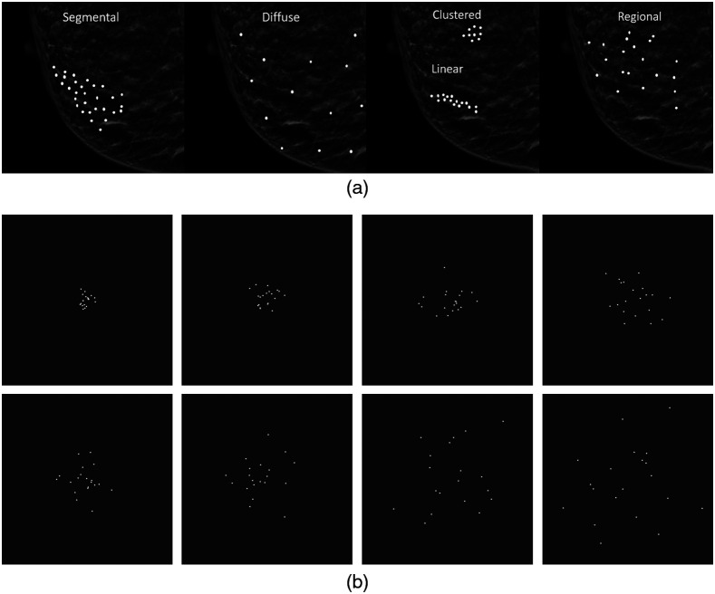
Identifying and classifying calcifications is challenging for various reasons such as the size of suspicious calcifications can be small ($<0.1\mathrm{mm}$⁷) making them difficult to perceive, differences in their distribution pattern can be extremely subtle, and technical factors can obscure their visibility. Once visualized, the crux of the radiologists’ visual task is to determine the calcifications’ morphology, distribution [see Fig 1(a)], location, and associated findings and then assign them a level of suspicion for malignancy, or a Breast Imagining-Reporting and Data System (BI-RADS) category. The BI-RADS is a method used to reduce inconsistencies in mammographic reports when classifying breast tissue density based on specific categories.⁸ The BI-RADS categories include category 0 (incomplete, additional imaging recommended), category 1 (negative), category 2 (benign lesions), category 3 (probably benign lesion, follow-up recommended), category 4 (suspicious lesions), and category 5 (highly suspicious lesion). The distribution of calcifications is a key component of the final BI-RADS category assessment and can lead to accurate, early breast cancer diagnosis or, conversely, missed diagnoses or unnecessary biopsy. At its root, this task is akin to determining the spread and elongation of a distribution of white dots. This exact visual task has been shown to lead to a considerable bias in perception: clusters of white dots [see Fig 1(b)] are judged to be more diffuse, or spread out, than their true distribution.⁹

Fig. 1.

Simulated examples of the five categories of calcification distributions on a background of (a) normal heterogeneously dense fibroglandular breast tissue and (b) examples of our experimental stimuli. In (b), the panels progress from the lowest level of spread (top left) to the highest level of spread (bottom right).

Characterizing a distribution of calcifications relies on visual processes known as ensemble perception. Ensemble perception refers to the processes by which the visual system quickly and efficiently integrates over a group of objects to compress information into one or more summary statistics, such as the mean or variability. For example, ensemble perception can detect the mean location, mean color, and mean size of a group of objects.^10–12 Most of the research on ensemble perception has focused on perception of the mean of the group (for review, see Ref. 13), but the perception of the variability or spread of the group is particularly relevant for the classification task faced by radiologists given that the visual system can detect the variability of a group of objects.¹⁴

Previously, we found that the perception of variability is considerably biased, with untrained individuals tending to overestimate the variability of items in a display by as much as 50% and more in displays with low variability.^15–17 In these experiments, student volunteers from a university introductory psychology course viewed a group of objects that varied along a single dimension (e.g., line orientation) and were required to judge the variability of this dimension in the display. In one study, the stimuli were sets of nine lines. Each line in the set differed in its orientation, and the sets differed from one another in the degree of their spread. The total spread across the lines was 9 deg for the lowest level of spread and 72 deg at the highest level of spread. At the lowest level of spread, the lines varied in orientation from each other by 1 deg for a total set variability of 9 deg, whereas at the highest level of spread, lines varied in orientation from each other by 8 deg for a total set variability of 72 deg (see Sec. 2). Each line in a set was presented sequentially, and for each set of lines, participants made a perceptual estimate of the spread. These judgments were transformed into bias scores that indicated the percent of overestimation in the spread of the lines. The bias scores were surprisingly large ($\sim 50\%$). In other words, participants perceived sets of lines with little spread as having considerably more spread. This visual bias found with lines is also present with a variety of other kinds of displays. Follow-up experiments revealed that the bias to overestimate the spread of a distribution was also found when judging items that varied in either color or size.^16,17 We will refer to the bias to overestimate the variability of a group of objects as the variability overestimation effect.

Breast cancer diagnoses require accurately classifying the distribution of calcifications, so the variability overestimation effect has the potential to negatively impact diagnostic accuracy. The presence of the effect would mean that distributions of calcifications that are more clustered (potentially suspicious) would be perceived as more regional or diffuse. Regional and diffuse distributions typically portend a benign diagnosis, so the variability overestimation effect could lead to an increased number of false-negative diagnoses. It is unclear, however, whether radiologists may be less prone to this bias given their expertise and enhanced training in identifying calcification distributions. The purpose of the present study is to test whether radiologists are also prone to the variability overestimation effect when making judgments about stimuli that resembled calcifications.

Given the possible outcome that radiologists do not show the variability overestimation effect with stimuli that are similar to calcifications, we also tested whether radiologists would show the effect in the context of stimuli that are unlike calcifications. The outcomes could be informative regarding whether expertise protects against the bias in general or only for previously trained stimuli. We choose to use the aforementioned line orientation task because the bias has already been demonstrated with this effect in university students and because the stimuli are unlike calcifications. The line orientation task and the dot task differ in many ways such as sequential versus simultaneous presentation and the number of objects in the set. These differences may be irrelevant: to preface our results, radiologists exhibited a bias to overestimate variability on both tasks, and the magnitude of the bias was similar to that found with untrained observers.

2. Method

We assessed variability perception in both expert radiologists and untrained observers in two tasks. One task required an assessment of the spread of white dots presented simultaneously on a dark background. The other task required assessing the variability of the orientation of lines presented sequentially. Whereas dot spread is relevant for diagnosing breast cancer, line orientation is irrelevant. We tested both tasks to assess whether expertise in one dimension had differential effects on the variability overestimation effect for relevant versus irrelevant dimensions.

2.1. Participants

We recruited 20 expert radiologists while they were attending the annual meeting of the Radiological Society of North America (RSNA). This conference hosts the Medical Image Perception Lab, which invites vision scientists to conduct research on expert radiologists who are willing to participate. On average, they had 11.25 years (median = 4, range = 0 to 52 years) of experience working as radiologists, with five identifying as female and 15 identifying as male. Only one did their fellowship training on the area of the breast, and 18 indicated that they read <200 mammograms per year. The percent of clinical time spent in breast imaging ranged from 0% to 35%, with over half the sample indicating that they spend at least some of their clinical time in breast imaging (see Table 1).

Table 1.

Overview of clinical time spent on breast imaging for radiologists in our study.

Percent of time	Number of radiologists
35%	1
20%	1
10%	2
5%	5
2%	1
6 ha	1
0%	7
No response	2

^aThis radiologist did not specify their answer in terms of a percentage.

For the untrained observers, 19 participants were recruited and completed the study through a crowdsourcing platform (Amazon’s Mechanical Turk; MTurk). It is worth noting that 34 started the study, but 11 incorrectly answered the catch question (see below) and did not finish the study, and four participants did not complete the experiment. These 15 participants were excluded.

Both groups of participants completed an online task to assess the variability overestimation effect with dots and with lines. The radiologists completed the task on iPads handed to them at the conference, and the untrained observers completed the survey on their own devices after signing up through MTurk. The protocol was deemed exempt by the Colorado State University Institutional Review Board given that no identifying information was collected, and the research involved an internet survey. With exempt protocols, informed consent is waived.

2.2. Stimuli

The stimuli were created in R.¹⁸ For the dot task, images of white dots presented at various levels of spread were presented one at a time [see Fig 1(b)]. The spread of the dots was manipulated across eight levels ranging from low spread to high spread. Dot placement was determined by randomly obtaining 10 or 20 samples from a normal distribution with a mean of zero and the standard deviation (SD) set to one of eight levels ranging from 0.25 to 2. The dots were placed on a $10\times 10$ (arbitrary units) space, corresponding to $600\times 600\text{pixels}$. The eight levels of spread were repeated for nine mean locations based on three lateral positions (left by 1 unit, center, and right by 1 unit) by three vertical positions (up by 1 unit, middle, and down by 1 unit). Vertical and lateral deviations were implemented to get participants to focus on spread, rather than a proxy for spread such as maximum height. There were 144 dot displays (eight levels of spread × two number of dots × nine mean locations).

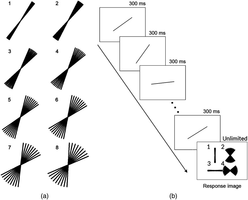
For the line task, the stimuli and materials were modeled after prior work.¹⁵ Animated GIFs that showed a sequence of nine lines, presented one at a time, were created. Each set consisted of nine lines that differed in orientation such that the mean orientation was either 35 deg or 55 deg and the spread among individual lines ranged from 1 deg to 8 deg. For the 1 deg spread, the consecutive line orientations differed by 1 deg; for the 2 deg range, the orientations differed by 2 deg, and so on [see Fig 2(a)]. Each set was presented as an animated GIF. The GIF started with a blank image for 300 ms, then showed each line one at a time for 300 ms each. The presentation order of the lines was randomized. After the presentation of the lines, another blank image was presented for 300 ms followed by the response image [see Fig 2(b)]. The response image remained visible until participants made their response. For each combination of mean angle and range, we created eight different animated GIFs, so each had a unique presentation order of the lines. There were a total of 128 animated GIFs (two mean angles × eight levels of spread × eight repetitions). All stimuli can be 186 freely viewed and downloaded at https://osf.io/gdth2/.

Fig. 2.

(a) Illustration of the eight line orientation ranges used in the line task. (b) Illustration of the sequence of presentation for the line orientation task. Each of the nine lines in the set was shown one at a time followed by the response image. The response image remained visible until the participant made their response.

2.3. Procedure

The experiment started with a welcome screen and then a question about the device being used (phone, tablet, or computer). Radiologists were then asked demographic questions and questions about whether their fellowship was in breast cancer, how many mammograms they read per year, and how much of their time is spent in breast imaging. Untrained observers were asked to select the fourth option as a simple catch trial. All 19 untrained observers who finished the experiment answered this question correctly.

Participants were randomly assigned to start with the dot task or start with the lines task. For the dot task, participants were told that they would see a display of dots and would have to make a judgment about their spread as being less or more spread out. They completed four practice trials, which consisted of one example of the lowest and highest levels of spread for each of the two sample sizes. Feedback was not provided. On each trial, including practice and test trials, the stimulus display remained until the participant indicated their response by selecting “less spread” or “more spread.” This kind of task is known as a bisection task for which participants compare what they see with an implicit mid-point, having first been trained on two anchor stimuli at the far extremes. Bisection tasks like this have been used to measure time perception in pigeons, mice, humans, and rats^19,20 and speed perception in humans.²¹ Participants completed 144 trials of the dot task. The trial order was randomized.

The line task was the same as in previous studies.¹⁵ Participants were told that they would see a set of lines that would be presented in the same location one at a time and presented at different orientations. They were told that they would then see four response options that varied in spread and would have to select the response image that looked most like what the lines would have looked like had they all been presented at once. This was also a bisection task with an implicit mid-point. In this task, the anchor levels of spread were presented on each trial as the response image. On each trial, they viewed one set of lines and selected one of the four options. These four choices allowed us to assess the perceived spread of the lines as well as the perceived mean, although we only analyzed the perceived spread given our research question. Participants completed 128 trials of the line task. The trial order was randomized.

3. Results

Bias in estimating spread was calculated for the dot task and the lines task. To calculate bias, we computed the points of subjective equality (PSE) for each task from the coefficients from general linear mixed models (GLMM) using the lme4 and lmerTest packages in R.^22,23 The PSE corresponds to the value of spread at which participants are equally likely to select more spread versus less spread. PSEs were transformed into bias scores to assess the extent to which spread was overestimated, underestimated, or accurately estimated. Participants with PSE scores beyond three times the interquartile range (IQR) were excluded from the analysis.

3.1. Dot Task

For the dot task, the positions of the dots were randomly sampled from normal distributions, so the sample SD and the population SD were highly correlated, $r=0.96$. We used the sample SD as the fixed effect in our analyses.

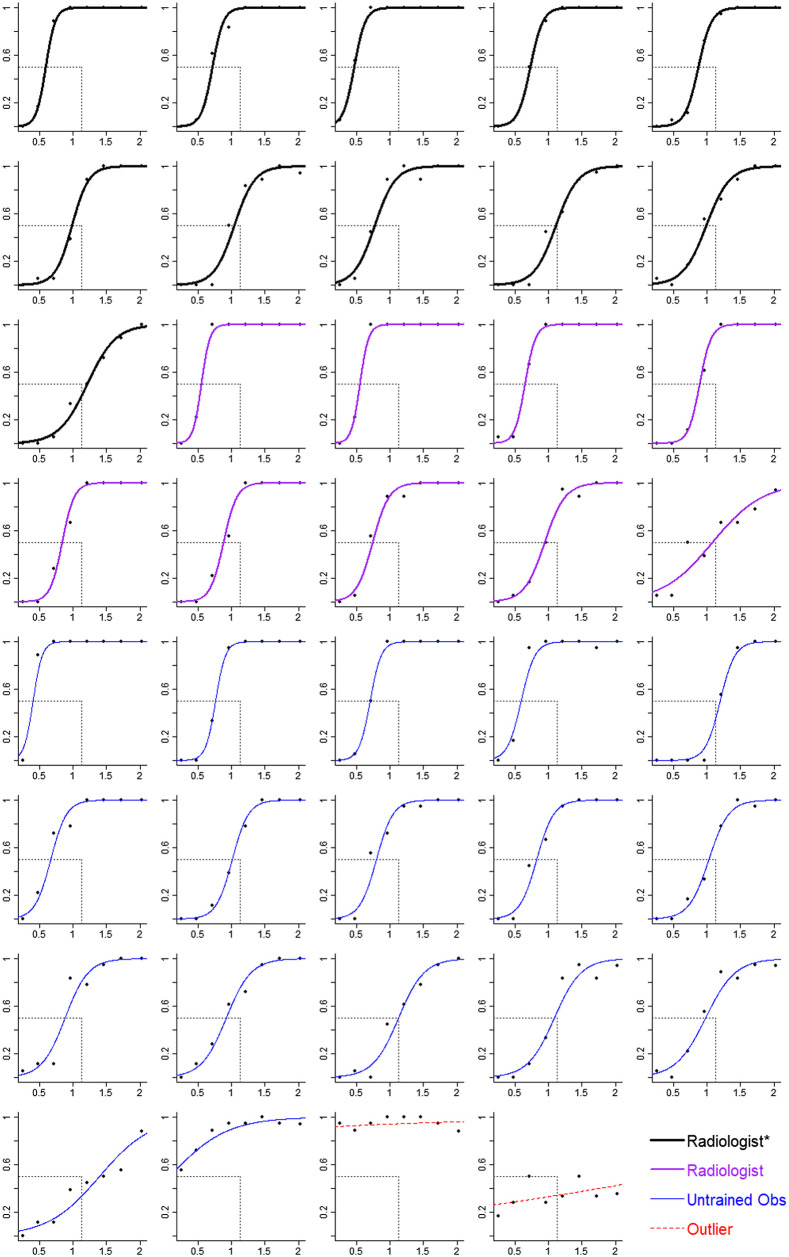
The data from the dot task were first assessed for outliers: two untrained observers had PSEs beyond three times the IQR (see Fig. 3) and were excluded from the analysis. The remaining data from the dot task were analyzed with a GLMM. The dependent measure was the response (coded as 0 for less spread and 1 for more spread). The fixed effects were the spread of the dots (SD, which was mean-centered), the number of dots (10, 20), and their interaction. Random effects including intercepts and slopes for dot spread were included for participants.

Fig. 3.

Estimated spread in the dot task as a function of SD of the dots for each participant. The $y$ axis is the proportion of trials for which the participant said the dots were more spread. The $x$ axis is the SD of the dots. Symbols correspond to mean estimates. Curves are logistic regressions based on the random effect coefficients from a GLMM. Participants are grouped by expertise. Thick black lines correspond to radiologists who spend at least some of their clinical time in breast imaging (radiologist*). Medium purple lines correspond to radiologists who spend no clinical time in breast imaging (radiologist). Thin blue lines correspond to untrained observers (untrained obs), and red dashed lines correspond to participants identified as outliers. The value of the SD of the dots at the point where the curve intersects the horizontal gray dashed line corresponds to the participant’s PSE. The vertical gray dashed line corresponds to the point of objective equality (POE), which is the SD of the dots that is equally less and more spread. Curves that intersect the horizontal line to the left of the vertical line indicate a bias to overestimate spread (top-left panel is one example). Curves that intersect the horizontal line at the vertical line indicate no bias (second row, fourth panel is one example).

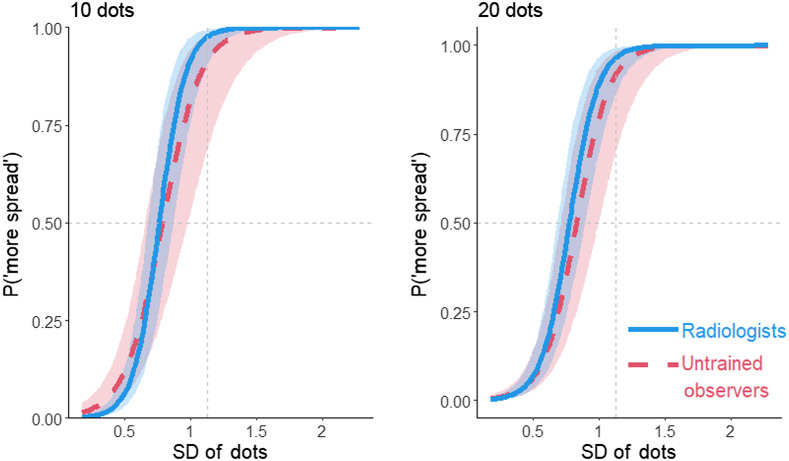
The model outcomes from the dot task are shown in Fig. 4. From the model, we then computed PSEs using the MixedPsy package.²⁴ This package provides 95% confidence intervals (CIs) via the bootstrap method, rather than calculating $p$-values. This is appropriate given that our focus is on estimating the magnitude of the bias and the uncertainty around this estimate. PSE scores were transformed into bias scores, which corresponded to the percent of overestimation.

Fig. 4.

The proportion of more spread responses in the dot task as a function of the SD of the dots, participant group, and number of dots (10,20). The vertical gray dashed line indicates the POE. Curves that intersect the horizontal gray dashed line to the left of the vertical dashed line show a bias to overestimate spread. Shading represents 95% CIs calculated from the model.

The bias score showed a 30% bias to overestimate the spread of the dots, 95% CI [21, 37%]. Out of the 37 participants, 33 (89%) overestimated the spread (see Fig. 5). The variability overestimation effect did not significantly differ between the radiologists and the untrained observers, $M_{\text{difference}}=-4\%$, 95% CI [−20%, 11%]. The bias was slightly larger when there were only 10 dots than when there were 20 dots for untrained observers, $M_{\text{difference}}=3\%$, 95% CI [0.2%, 6%], and for radiologists, $M_{\text{difference}}=2\%$, 95% CI [0.2%, 5%] (Fig. 6). The data indicate that perceptual processes exaggerate the amount of spread seen in the display.

Fig. 5.

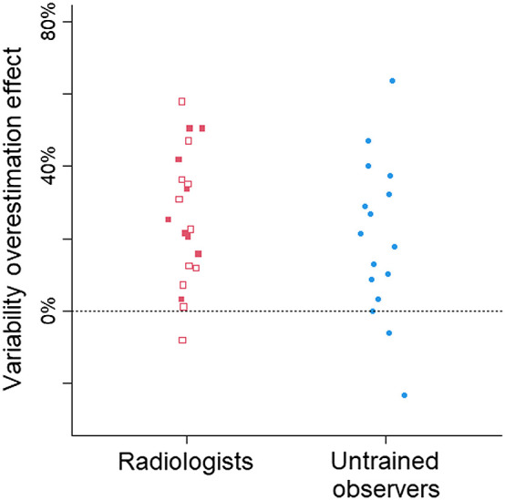
The variability overestimation effect in the dot task, collapsed across number of dots and grouped by participant group. Each symbol corresponds to the bias in one participant. Open symbols correspond to radiologists who spend at least some of their clinical time on mammograms. The horizontal dashed line at 0 indicates no bias. Positive scores indicate a bias to overestimate the spread of the dots, and negative scores indicate a bias to underestimate.

Fig. 6.

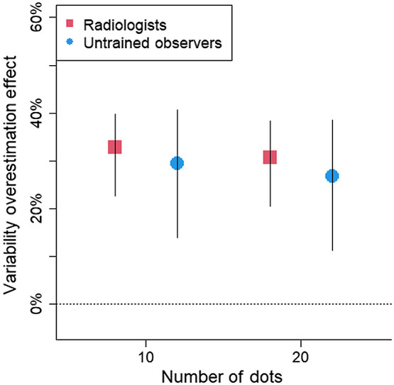
Estimated variability overestimation effect (as % overestimation) in the dot task as a function of participant group and number of dots. The horizontal dashed line at 0 indicates no bias. Positive scores indicate a bias to overestimate the spread of the dots. Error bars represents 95% CIs.

Another outcome is the extent to which participants were sensitive to the spread of the dots. Sensitivity and bias are separate ways to describe performance. Sensitivity refers to the ability to discriminate between different levels of spread, whereas bias refers to their tendency to see or judge the dots as being more spread out. Sensitivity can be quantified as the slopes from the model, with steeper slopes indicating better sensitivity to the spread of the dots whereas flat slopes indicate no sensitivity (see Fig. 4). In psychophysics, it is more typical to quantify sensitivity as the just-noticeable difference (JND). The JND is the amount of change needed in the spread of the dots for that difference in spread to be noticeable, which is defined as shifting responses from 50% (chance) to 75%.

The JNDs were smaller, indicating better sensitivity to the spread of the dots, for the radiologists than for the untrained observers, $M_{\text{radiologist}}=0.11$, 95% CI [0.10, 0.15], $M_{\text{untrained observers}}=0.15$, 95% CI [0.12, 0.22], $M_{\text{difference}}=0.03$, 95% CI [−0.01, 0.10]. Although the 95% CI of the difference overlapped zero, the radiologists showed 31% greater sensitivity compared with the untrained observers. Perhaps with larger samples sizes, this difference would have been statistically significant; however, we cannot determine whether the better performance by radiologists was due to their expertise versus an alternative explanation such as motivation when completing the task. Of note, even though radiologists showed greater sensitivity to the spread of the dots, they were still prone to the variability overestimation effect.

3.2. Line Task

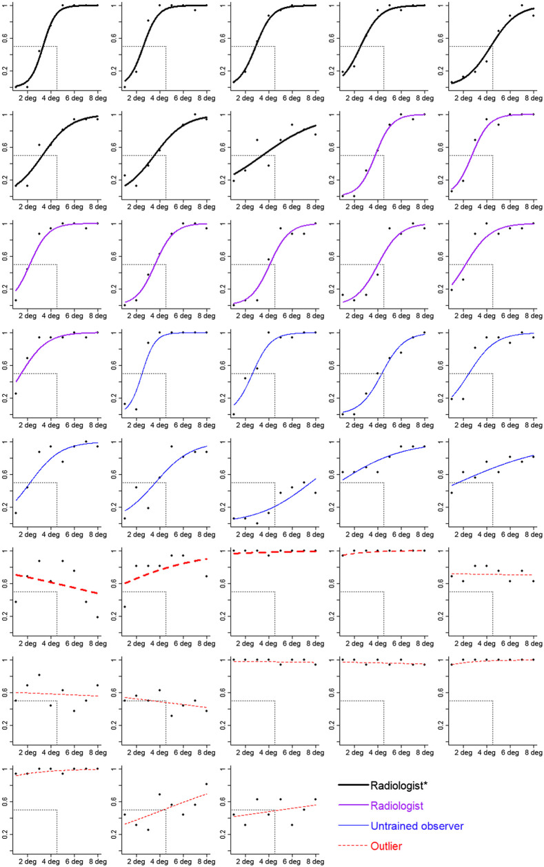
Responses were re-coded with selections of the less spread choices being coded as 0 and selections of the more spread choices coded as 1. A GLMM with the spread of the line orientations as the fixed effect was run to identify outliers. Outliers were identified as participants who had a PSE beyond 3 times the IQR, had flat slopes, or whose data did not appear to be well fit by the model (assessed visually). Together, 13 participants were identified as outliers (nine untrained observers, four radiologists; see Fig. 7). Although this is a high number of outliers, previous research with this task has also shown high rates of outliers.¹⁵ Data loss is not a concern for statistical power because the variability overestimation effect with line orientation is quite large. The effect size is estimated to be $d>1.20$.¹⁵ A power analysis indicates that, to achieve 80% power to detect the variability overestimation effect estimated at $d=1.20$, only eight participants are needed. We analyzed the data from 16 radiologists and nine novices.

Fig. 7.

Estimated spread in the line task as a function of spread of the lines for each participant. The $y$ axis is the proportion of trials for which the participant said the dots were more spread. The $x$ axis is the spread of the lines (in units of degrees between closest lines). Symbols correspond to mean estimates. Curves are logistic regressions based on the random effect coefficients from a GLMM. Participants are grouped by expertise. Thick black lines correspond to radiologists who spend at least some of their clinical time in breast imaging (radiologist*). Medium purple lines correspond to radiologists who spend no clinical time in breast imaging (radiologist). Thin blue lines correspond to untrained observers (untrained obs), and red dashed lines correspond to participants identified as outliers (with thickness corresponding to expertise). The value of the spread of the lines at the point where the curve intersects the horizontal gray dashed line corresponds to the participant’s PSE. The vertical gray dashed line corresponds to the POE, which is the spread of the lines that is equally less and more spread. Curves that intersect the horizontal line to the left of the vertical line indicate a bias to overestimate spread (top-left panel is one example). Curves that intersect the horizontal line at the vertical line indicate no bias (first row, last panel is one example).

To calculate bias scores for the line task, we ran a GLMM with estimated spread (coded as 0 for less spread and 1 for more spread) as the dependent measure. The fixed effects were the spread of the line orientations, group (radiologists or untrained observers), and their interaction. Random effects for participant included intercepts and slopes for the main effect of the spread. The model outcomes are shown in Fig. 8. The model coefficients were used to calculate bias scores and JNDs.

Fig. 8.

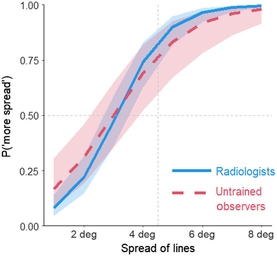
Estimated spread in the line task as a function of the spread of the lines (in degrees) and participant group. Shading represents 95% CIs calculated from the model.

Overall, participants overestimated the spread of the line orientations by 31%, 95% CI [22%, 41%]. Out of 27 participants, 26 (96%) overestimated the spread of the lines. Both radiologists and untrained observers overestimated the spread of the line orientations by 31% and 33%, respectively; 95% CI for radiologists [21%, 41%]; 95% CI for untrained observers [15%, 49%]. The difference in the bias between the two participant groups was 2%, 95% CI of the difference $[-17\%,2\%]$.

As with the dots, radiologists were more sensitive to the variability in the orientation of the lines compared with untrained observers. The mean JND for line orientation spread for the radiologists was 0.95 deg, 95% CI [0.82 deg, 1.23 deg]. This means that the spread of the lines had to increase by nearly 1 deg for the radiologists to notice the difference in spread. The mean JND for the untrained observers was 1.37 deg, 95% CI [1.02 deg, 2.16 deg]. Although the difference in JNDs was notable with radiologists being 44% more sensitive compared with untrained observers, the 95% CIs for the difference overlapped 0, $M_{\text{difference}}=0.42$, 95% CI $[-0.02,1.46]$. Even with the radiologists potentially being more sensitive to the spread of the lines, they showed a similar magnitude of the variability overestimation effect compared with the untrained observers.

4. Discussion

Correctly categorizing the distribution of calcifications is a crucial visual task in the early detection of breast cancer. Because it is a visual task, performance may be susceptible to errors due to visual biases. Potentially relevant is the bias to overestimate the variability of a set of objects such as the positions of a set of dots or orientations of a set of lines.^9,15 This bias is called the variability overestimation effect. The current research validates the possibility that this visual bias could impede diagnostic accuracy by demonstrating that expert radiologists are also prone to this bias. They overestimated the distributions of dots that resembled calcifications by 32%. This validates the concern that the variability overestimation effect could impede diagnostic accuracy when reading breast mammography by leading radiologists to perceive a distribution of dots as more spread, resulting in more false-negative results.

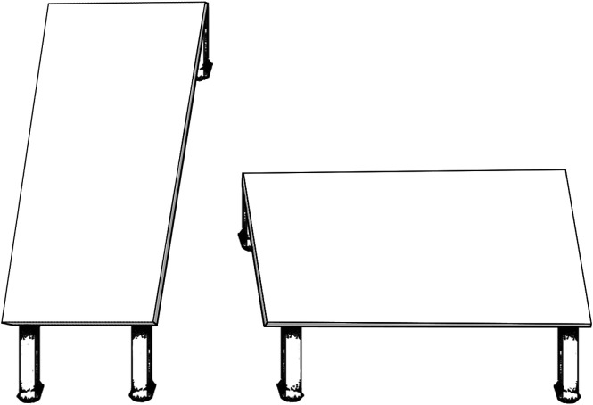
The variability overestimation effect was present and of similar magnitudes for radiologists and untrained observers. The lack of difference across levels of expertise suggests a universal visual bias, rather than something that can be eliminated via training. Visual biases such as classic visual illusions such as the Shepard’s table illusion²⁵ (see Fig. 9) have the property of being cognitively impenetrable. This means that, once you know the tabletop shapes are the same as each other (measure for yourself!), this knowledge does not eliminate or even lessen the illusion. Visual biases can be robust and difficult to eradicate.

Fig. 9.

Shepard’s table illusion.

4.1. Limitations and Future Directions

We highlight a few limitations with the current experiments. Although the dots bore some resemblance to calcifications, the task was not presented as a breast cancer screening task nor a simulation. Future work could assess whether this same bias would occur in a more realistic breast cancer screening task. Another limitation is the lack of radiologists in the study who primarily focus on breast imaging. Future studies could determine whether radiologists with more expertise in breast imaging are also susceptible to the bias. Finally, future work could explore the impact that providing explicit feedback on variability judgments has on the magnitude of the bias. This would indicate whether training programs could help mitigate or lessen the variability overestimation effect and its potential role in misdiagnoses.

5. Summary

The variability overestimation effect is a potential problem for classifying distributions of calcifications when diagnosing breast cancer (see Fig. 1). Calcifications with more clustered distributions may be misperceived as being more regional or diffuse. The errors produced by the variability overestimation effect could lead to false-negative diagnoses, and a breast cancer may go undetected.

Biographies

Jessica K. Witt is a professor of psychology at Colorado State University. She received her BA degree in computer science and psychology from Smith College and her MA degree and PhD in psychology from the University of Virginia. She is the recipient of early career awards from the Association for Psychological Science, the American Psychological Association, and the Psychonomic Society. Her research interests include visual biases and assessing sensitivity and bias in visual displays of quantitative information.

Amelia C. Warden is a graduate student in the Department of Psychology at Colorado State University. She received her BS degree in cognitive science from the University of Kansas, her MS degree in experimental psychology from the University of Idaho, and her MFA from Washington State University. Her research specialty is in human factors.

Michael D. Dodd is a professor of psychology at the University of Nebraska—Lincoln. He received his BSc degree in psychology from Trent University and his MA degree and PhD in psychology from the University of Toronto. His research specialty is in visual attention.

Elizabeth E. Edney is an assistant professor of radiology at the University of Nebraska Medical Center. She received her BA degree in history from Creighton University and her MD degree from Creighton University School of Medicine. Her specialty is in abdominal imaging and breast imaging.

Disclosures

The authors have no relevant financial interests in the manuscript and no other potential conflicts of interest to disclose.

Code, Data, and Materials Availability

Stimuli, data, and analysis scripts are freely available at https://osf.io/gdth2/.

References

- 1.Chaudhury S., et al. , “Breast cancer calcifications: identification using a novel segmentation approach,” Comput. Math. Methods Med. 2021, 9905808 (2021). 10.1155/2021/9905808 [DOI] [PMC free article] [PubMed] [Google Scholar] [Retracted]
- 2.Durand M. A., et al. , “False-negative rates of breast cancer screening with and without digital breast tomosynthesis,” Radiology 298(2), 296–305 (2021). 10.1148/radiol.2020202858 [DOI] [PubMed] [Google Scholar]
- 3.Huynh P. T., Jarolimek A. M., Daye S., “The false-negative mammogram,” Radiographics 18(5), 1137–1154 (1998). 10.1148/radiographics.18.5.9747612 [DOI] [PubMed] [Google Scholar]
- 4.Ekpo E. U., Alakhras M., Brennan P., “Errors in mammography cannot be solved through technology alone,” Asian Pac. J. Cancer Prevent. 19(2), 291 (2018). 10.22034/APJCP.2018.19.2.291 [DOI] [PMC free article] [PubMed] [Google Scholar]
- 5.Bent C. K., et al. , “The positive predictive value of BI-RADS microcalcification descriptors and final assessment categories,” Am. J. Roentgenol. 194(5), 1378–1383 (2010). 10.2214/AJR.09.3423 [DOI] [PubMed] [Google Scholar]
- 6.Horvat J. V., et al. , “Calcifications at digital breast tomosynthesis: imaging features and biopsy techniques,” Radiographics 39(2), 307–318 (2019). 10.1148/rg.2019180124 [DOI] [PMC free article] [PubMed] [Google Scholar]
- 7.Wilkinson L., Thomas V., Sharma N., “Microcalcification on mammography: approaches to interpretation and biopsy,” Br. J. Radiol. 90(1069), 20160594 (2017). 10.1259/bjr.20160594 [DOI] [PMC free article] [PubMed] [Google Scholar]
- 8.Orel S. G., et al. , “BI-RADS categorization as a predictor of malignancy,” Radiology 211(3), 845–850 (1999). 10.1148/radiology.211.3.r99jn31845 [DOI] [PubMed] [Google Scholar]
- 9.Witt J. K., Fu M., Dodd M. D. (under review), Variability of object locations is overestimated.
- 10.Ariely D., “Seeing sets: representation by statistical properties,” Psychol. Sci. 12(2), 157–162 (2001). 10.1111/1467-9280.00327 [DOI] [PubMed] [Google Scholar]
- 11.Sun P., et al. , “Human attention filters for single colors,” Proc. Natl. Acad. Sci. U. S. A. 113(43), E6712–E6720 (2016). 10.1073/pnas.1614062113 [DOI] [PMC free article] [PubMed] [Google Scholar]
- 12.Maule J., Witzel C., Franklin A., “Getting the gist of multiple hues: metric and categorical effects on ensemble perception of hue,” J. Opt. Soc. Am. A 31(4), A93–A102 (2014). 10.1364/JOSAA.31.000A93 [DOI] [PubMed] [Google Scholar]
- 13.Whitney D., Yamanashi Leib A., “Ensemble perception,” Annu. Rev. Psychol. 69, 105–129 (2018). 10.1146/annurev-psych-010416-044232 [DOI] [PubMed] [Google Scholar]
- 14.Morgan M. J., Chubb C., Solomon J. A., “A “dipper” function for texture discrimination based on orientation variance,” J. Vision 8(11), 9 (2008). 10.1167/8.11.9 [DOI] [PMC free article] [PubMed] [Google Scholar]
- 15.Witt J. K., “The perceptual experience of variability in line orientation is greatly exaggerated,” J. Exp. Psychol. Hum. Percept. Perform. 45(8), 1083–1103 (2019). 10.1037/xhp0000648 [DOI] [PubMed] [Google Scholar]
- 16.Witt J. K., Dodd M. D., Edney E., “The perceptual experience of orientation variability,” J. Vision 19(10), 193a (2019). 10.1167/19.10.193a [DOI] [Google Scholar]
- 17.Warden A. C., et al. , “Overestimation of variability in ensembles of line orientation, size and color,” J. Vision 20(11), 1240 (2020). 10.1167/jov.20.11.1240 [DOI] [Google Scholar]
- 18.R Core Team, R: A Language and Environment for Statistical Computing, R Foundation for Statistical Computing; (2019). [Google Scholar]
- 19.Penney T. B., Gibbon J., Meck W. H., “Categorical scaling of duration bisection in pigeons (Columba livia), mice (Mus musculus), and humans (Homo sapiens),” Psychol. Sci. 19(11), 1103–1109 (2008). 10.1111/j.1467-9280.2008.02210.x [DOI] [PubMed] [Google Scholar]
- 20.Raslear T. G., “Perceptual bias and response bias in temporal bisection,” Percept. Psychophys. 38(3), 261–268 (1985). 10.3758/BF03207153 [DOI] [PubMed] [Google Scholar]
- 21.Witt J. K., Sugovic M., “Performance and ease influence perceived speed,” Perception 39(10), 1341–1353 (2010). 10.1068/p6699 [DOI] [PubMed] [Google Scholar]
- 22.Bates D., et al. , “Fitting linear mixed-effects models using lme4,” J. Stat. Software 67(1), 1–48 (2015). 10.18637/jss.v067.i01 [DOI] [Google Scholar]
- 23.Kuznetsova A., Brockhoff P. B., Christensen R. H. B., “lmerTest package: tests in linear mixed effects models,” J. Stat. Software 82(13), 1–26 (2017). 10.18637/jss.v082.i13 [DOI] [Google Scholar]
- 24.Moscatelli A., Mezzetti M., Lacquaniti F., “Modeling psychophysical data at the population-level: the generalized linear mixed model,” J. Vision 12(11), 26 (2012). 10.1167/12.11.26 [DOI] [PubMed] [Google Scholar]
- 25.Shepard R. N., Mind Sights: Original Visual Illusions, Ambiguities, and Other Anomalies, with a Commentary on the Play of Mind in Perception and Art, WH Freeman/Times Books/Henry Holt & Co; (1990). [Google Scholar]