Decomposition of Two-Component Ultrasound Pulses in Cancellous Bone Using Modified Least Squares Prony’s Method – Phantom Experiment and Simulation

Abstract

Porous media such as cancellous bone often support the simultaneous propagation of two compressional waves. When small bone samples are interrogated in through-transmission with broadband sources, these two waves often overlap in time. The Modified Least-Squares Prony’s (MLSP) method was tested for decomposing a 500 kHz-center-frequency signal containing two overlapping components: one passing through a polycarbonate plate (to produce the “fast” wave) and another passing through a cancellous-bone-mimicking phantom (to produce the “slow” wave). The MLSP method yielded estimates of attenuation slopes accurate to within 7% (polycarbonate plate) and 2% (cancellous bone phantom). The MLSP method yielded estimates of phase velocities accurate to within 1.5% (both media). The MLSP method was also tested on simulated data generated using attenuation slopes and phase velocities corresponding to bovine cancellous bone. Throughout broad ranges of signal-to-noise ratio (SNR) and fast-slow-wave-velocity differential, the MLSP method yielded estimates of attenuation slope that were accurate to within 10% and estimates of phase velocity that were accurate to within 5% (fast wave) and 2% (slow wave).

INTRODUCTION

Ultrasound devices are increasingly used to characterize cancellous bone (Laugier, 2008). Most cancellous bone devices target the calcaneus. Recent developments include increased portability (Kaufman et al., 2007), expansion to new sites such as the radius (Le Floch et al., 2008), and a dual-frequency pulse-echo method for removing effects of soft tissues (Riekkinen et al., 2006, 2008). A greater understanding of the mechanisms underlying the interaction between ultrasound and bone could lead to improved diagnostic devices. Cancellous bone consists of a porous mineralized trabecular network with a fluid filler (marrow in vivo or water in vitro). Many investigators have reported experimental evidence that compressional waves incident upon cancellous bone samples in vitro can produce two compressional waves propagating in the sample (Hosokawa and Otani 1997, 1998; Hughes et al. 1999; Kaczmarek et al. 2002; Cardoso et al. 2003; Mizuno et al., 2008). The existence of two compressional waves in porous media is predicted by Biot theory (Biot 1956a, 1956b, 1956c, 1962, 1963), which has been applied to bone by many investigators (McKelvie and Palmer 1991; Williams 1992; Hosokawa and Otani 1997, 1998; Haire and Langton 1999; Hughes et al. 2003; Lee et al. 2003; Mohamed et al. 2003; Cardoso et al. 2003; Fellah et al. 2004; Wear et al. 2005; Lee and Yoon 2006; Hughes et al. 2007; Pakula et al. 2008; Fellah et al. 2008; Sebaa et al. 2008). Within the Biot theory, two compressional waves correspond to the fluid and solid moving in-phase (fast wave) and out-of-phase (slow wave) with each other.

Several reports suggest that separation of composite pulses into their two compressional components provides useful information regarding the interaction of ultrasound with cancellous bone samples:

1. Measurements on cancellous bone samples in vitro suggest that the fast wave exhibits a different dependence of attenuation coefficient on frequency than the slow wave (Hosokawa and Otani 1997; Kaczmarek et al. 2002; Cardoso et al. 2003).

2. An extension of Biot theory suggests that the relative amplitudes of fast and slow waves are sensitive to bone volume fraction, sample thickness, tortuosity, and viscous characteristic length (Fellah et al. 2004).

3. Three-dimensional finite-difference time-domain simulations suggest that fast wave velocity is much more sensitive to bone volume fraction than slow wave velocity (Haïat et al. 2008; Hosokawa 2008) and that fast and slow wave attenuation coefficients exhibit markedly different dependencies on bone volume fraction (Hosokawa 2008).

In addition, fast wave speed in bovine cancellous bone has been shown to depend on structural anisotropy and to be maximum when propagation is parallel to the trabecular orientation (Mizuno et al., 2008).

Unfortunately, separate analysis of fast and slow waves is complicated by the fact that the two pulses often overlap in time due to a combination of 1) insufficient contrast between fast and slow wave velocities and 2) insufficient sample thickness. The contrast between fast and slow velocities is lower when the ultrasound propagation direction is perpendicular (compared with parallel) to the predominant trabecular orientation (Hosokawa and Otani 1997, 1998). In addition, the degree of structural anisotropy influences the temporal separability of fast and slow waves (Haïat et al. 2008). Situations when pulses contain overlapping fast and slow wave components may be identified by assessing the correlation coefficient of a least-squares linear fit between transmission signal loss and frequency. A low correlation coefficient may be an indication of interference between fast and slow waves (Haïat et al. 2008). Moreover, low correlations can result from multi-mode signals that may not be the result of Biot-type phenomena, for example, signals containing multi-path effects. In addition, detection of two waves becomes more difficult when the amplitude of one wave is significantly larger than the amplitude of the other wave.

A Bayesian method has been shown to be effective for separation of overlapping time-domain pulses for simulated signals mimicking measurements from cancellous bone (Marutyan et al. 2006). This method involves calculations using Markov chain Monte Carlo with simulated annealing. It may not be practical for many researchers since the computer code is extremely complicated and the processing time can be lengthy (100 minutes on a Sun Enterprise 250 dual 400-MHz workstation) unless a cluster of processors is used (3 minutes using 32 processors on an SGI Altix 3000 with Itanium2 processors running at 900 MHz) (Marutyan et al. 2007).

In the present paper, the Modified Least-Squares Prony (MLSP) method is applied in frequency domain to the transfer function of the two-wave-generating experiment. The MLSP method models a signal as a sum of exponentially-damped sinusoids and recovers four parameters for each component (amplitude, decay rate, oscillation rate, and initial phase). It may be applied to cancellous bone because the transfer function that describes transmission through cancellous bone may be represented as a sum of exponentially-damped sinusoids.

THEORY

Two-wave model

The model used here is adapted from a previous model (Marutyan et al., 2006) for composite media such as cancellous bone that exhibit two waves propagating simultaneously through a linear-with-frequency attenuating medium:

$$output(\omega )=input(\omega )\lfloor H_{fast}(\omega )+H_{slow}(\omega )\rfloor$$ (1)

where

$$H_j(\omega )=A_j\exp [-{\alpha }_j(\omega )d]\exp \left[i\omega \frac{d}{v_j(\omega )}\right]\exp \left[-i\omega \frac{d}{c}\right],$$ (2)

ω = 2πf	and f is the ultrasound frequency,
Aj	includes the effects of transmission through boundaries,
αj(ω) =	attenuation coefficient = βj ω / 2π,
βj =	attenuation slope
vj(ω) =	phase velocity,
d =	sample thickness,
c =	speed of sound in water,

and j stands for either fast or slow.

One difference between this model and the previous model (Marutyan et al., 2006) is the inclusion of the last exponential factor, exp[-i ωd/c], which explicitly accounts for the fact that, in a substitution experiment, the attenuating sample replaces an equivalent length of water in the acoustic beam path. Both models neglect diffraction effects in the substitution experiment that can be significant when the thickness and sound speed contrast between the reference and experimental media are sufficiently great (Kaufman et al., 1995), but are typically small for cancellous bone samples (Kaufman et al., 1995; Droin et al., 1998).

Prony’s Method and Variants

Prony’s method and its variants model a digitized complex signal, x[1], x[2], x[3], …, x[N], as the sum of p exponentially-damped sinusoids as follows (Marple 1987):

$$x[n]=\sum _{j=1}^p{A}_j\exp [(s_j+i2\pi q_j)(n-1)\text{Δ}\omega +i{\theta }_j]$$ (3)

where A_j is an amplitude, s_j is a damping rate, q_j is an oscillation rate, and θ_j is an initial phase of the j^th complex exponential. Δω is the sample interval. In Equation 3, Marple’s notation has been modified in order to reduce confusion that may arise from the fact that while the most common application of Prony’s method and its variants is modeling a time domain signal, the present application is modeling a frequency domain signal.

By comparing Equation 3 with Equations 1 and 2, the following correspondences can be made:

p = 2,

ω = (n-1) Δω,

s_j = - β_j d / 2π,

$q_j=\frac{d}{2\pi }\left[\frac{1}{v_j({\omega }_0)}-\frac{1}{c}\right]$, and

θ_j = 0 (with no loss in generality if A_j are allowed to be complex).

In Equation 3, the frequency-dependence of phase velocity, v_j(ω), has been ignored so that v_j(ω) ≈ v_j(ω₀) where ω₀ = 2πf₀ and f₀ is a reference frequency such as the transducer center frequency. In other words, dispersion of the fast and slow wave components has been ignored. The experiment and simulation described below will test this approximation for examples relevant to cancellous bone. Apparent dispersion of the composite signal, which can result from the interference between the fast and slow waves (Bauer et al., 2008), will not necessarily be zero in this model. Moreover, as explained in the Discussion section, frequency-dependent phase velocity of fast and slow waves may be computed from MLSP-method-based estimates of attenuation slopes and phase velocities at the reference frequency.

Prony’s method and its variants have been described in great detail elsewhere (Marple, 1987). Prony’s original method was designed for cases when the number of data points equals the number of parameters to be estimated. In this case, an exact fit of the model to the data may be performed. When the number of data points exceeds the number of parameters to be estimated, the MLSP method may be used to generate an approximate fit of the model to the data. Prony’s method and its variants consist of three steps. First, the data are fit to a linear prediction model. Then, estimates for damping rates and oscillation rates are obtained from the roots of a polynomial formed from the linear prediction coefficients obtained in step 1. Finally, estimates for amplitudes and initial phases are obtained from the solution of a set of linear equations. For more detail, see (Marple 1987).

MATERIALS AND METHODS

Data Acquisition

The MLSP method to estimate parameter values in Equations (1) and (2) may be tested on experimental data acquired from composite specimens, such as cancellous bone samples, with known parameter values (i.e. attenuation slope and phase velocity) for both fast and slow waves. However, it can be difficult to find or produce composite specimens in which these parameter values are known with great certainty. Therefore, in the present study, a simplified but mathematically equivalent experiment was performed as follows. First, a through-transmission measurement was performed through a 2.5-cm-thick polycarbonate plate. Second, a through-transmission measurement was performed through a 3.6-cm-thick cancellous bone phantom (Model 063 CIRS Inc., Norfolk, VA, USA). The phantom consisted of a block of homogeneous proprietary urethane material that mimicked the frequency-dependent attenuation and sound speed, but not the micro-architecture, of cancellous bone. Third, the digitized radio-frequency (RF) signals from the two measurements were added in software in order to simulate a measurement that would be obtained from a composite medium. Finally, a through-transmission calibration measurement through a water-only path was measured.

A pulser/receiver (5077PR, Panametrics, Waltham, MA, USA) and a pair of coaxially-aligned, 500 kHz, broadband, 1” (2.5 cm) diameter, 1.5” (3.8 cm) focal length transducers (Panametrics, V301, Waltham, MA, USA) were used to interrogate samples in a water tank. The propagation path between transducers was twice the focal length. Received RF signals were digitized (8 bit, 25 MHz) using an oscilloscope (LeCroy, 9310C, Chestnut Ridge, NY, USA) and stored on computer (via general purpose interface bus) for off-line analysis.

Data Analysis

Spectra for each of the four signals (i.e. 1: polycarbonate plate signal, 2: cancellous bone phantom signal, 3: sum of polycarbonate plate signal plus cancellous bone phantom signal, and 4: pure water signal) were computed using Fast Fourier Transforms (FFT’s). The ratio of the spectrum from the polycarbonate plate to the spectrum from a water-only path yielded H_fast(ω) (see Equation 1). The ratio of the spectrum from the cancellous bone phantom to the spectrum from a water-only path yielded H_slow(ω). The ratio of the spectrum from the summed signal (polycarbonate signal plus cancellous bone phantom signal) to the spectrum from a pure water path yielded H_total(ω).

Values for attenuation slopes and phase velocities were obtained by applying the MLSP method directly to H_total(ω). In order to assess the accuracy of the MLSP method, these values were compared to values for attenuation slopes and phase velocities obtained directly from H_fast(ω) and H_slow(ω) using the following conventional methods.

Attenuation coefficients, α_j(ω), were estimated using a log spectral difference technique (Kuc and Schwartz 1979).

$${\alpha }_j(\omega )=\frac{1}{d}\left[10\log S_w(\omega )-10\log S_j(\omega )\right]$$ (4)

where S_w(ω) is the spectrum from a water-only path and S_j(ω) is the spectrum from either the polycarbonate plate or the cancellous bone phantom. Since the attenuation coefficients for both the polycarbonate plate and the cancellous bone phantom were very nearly linear with frequency, they could be accurately characterized by the slope of a least-squares linear fit of attenuation coefficient (dB/cm) vs. frequency over the range from 0.20 to 0.65 MHz.

Frequency-dependent phase velocities, v_j(ω), were computed using

$$v_j(\omega )=\frac{c}{1+\frac{c\text{Δ}\varphi (\omega )}{\omega d}}$$ (5)

where Δϕ(ω) is the difference in unwrapped phases (see next paragraph) of the received signals with and without the sample in the water path, d is the sample thickness, and c is the temperature-dependent speed of sound in distilled water given by (Kaye and Laby, 1973)

$$c=1402.9+4.835T-0.047016T^2+0.00012725T^{3}m/s$$ (6)

and T is the temperature in degrees Celsius. The equation for phase velocity (Equation 5) is often reported with a minus sign instead of a plus sign in the denominator. The ambiguity arises from ambiguity in Δϕ(ω), which may be computed as ϕ(ω) - ϕ_w(ω) or ϕ_w(ω) - ϕ(ω). Temperature, measured with a digital thermometer, was 19.9° for these measurements, which meant that c was about 1482 m/s.

The unwrapped phase difference, Δϕ(ω), was computed as follows. FFT’s of the digitized received signals were taken. The phase of the signal at each frequency was taken to be the inverse tangent of the ratio of the imaginary to real parts of the FFT at that frequency. Since the inverse tangent function yields principal values between -π and π, the phase had to be unwrapped by adding an integer multiple of 2π to all frequencies above each frequency where a discontinuity appeared.

Simulation

A simulation was performed in order to evaluate the MLSP method for fast and slow wave parameters reported for bovine cancellous bone. Simulated waveforms were generated using Equations (1) and (2). The parameters of the waveforms were d = 1 cm, A_fast = 0.75, A_slow = 0.25, β_fast = 20 dB/cmMHz, β_slow = 6.9 dB/cmMHz, v_fast(ω₀) = 1550, 1600, 1700, 1800, 1900, 2000, and 2100 m/s, and v_slow(ω₀) = 1500 m/s (Hosokawa and Otani 1997; Waters and Hoffmeister 2005; Anderson et al. 2008) where ω₀ = 2πf₀ and f₀ = 1 MHz. The sample thickness and fast wave velocities were restricted to relatively small values in order to ensure temporal overlap between fast and slow waves. (If fast and slow waves do not overlap, then the task of measuring separate fast and slow wave properties is trivial.) Frequency-dependent fast and slow wave velocities were generated from (Anderson et al. 2008)

$$v_j(\omega )=v_j({\omega }_0)+v_j{({\omega }_0)}^2\frac{{\beta }_j}{{\pi }^2}\ln \left(\frac{\omega }{{\omega }_0}\right).$$ (7)

Gaussian white noise was added to the RF waveforms to generate signals with signal-to-noise ratios (SNR’s) ranging from 20 to 60 dB. SNR was defined as the ratio of the amplitude of the signal pulse to the amplitude of the Gaussian white noise. The input signal, input(ω) in Equation 1, was a Gaussian function, exp[-(f-f₀)² / 2σ²] with f₀ = 1 MHz and σ = 0.2 MHz. Simulated RF signals and spectra were analyzed in a manner similar to that described above for experimental data. The MLSP method was applied to the ratio of output to input spectra over the range from 0.5 to 1.5 MHz. Six hundred trials were generated for each value of SNR. Previous investigators have shown that in the presence of noise, biases in parameter estimates may be reduced by selecting model orders higher than the number of exponentials actually in the signal (Van Blaricum and Mittra, 1975; Kumaresan and Tufts, 1982; Marple, 1987). This is reasonable because the model should be able to accommodate not only the energy in the signal but also the energy in the noise as well. Model orders for values of p = 2, 3, 4, 5, and 6 were applied to each waveform. For p > 2, the two waves with maximum total energy were designated as the two signal waves. The wave with the faster velocity was designated as the fast wave, H_fast(ω), and the wave with the slower velocity was designated as the slow wave, H_slow(ω). The model estimate was the sum of the two highest energy waves, H_fast(ω) + H_slow(ω). The order (p) that produced the minimum final prediction error (FPE) between the model and the simulated H(ω) was designated as the optimum order, where

$$FPE={\rho }_p\left(\frac{N+(p+1)}{N-(p+1)}\right),$$ (8)

ρ_p is the prediction error power, and N is the number of samples in the estimate for H(ω) (Marple, 1987). The means and standard deviations for the parameter (amplitude, attenuation slope, and phase velocity) estimates were computed for each value of SNR.

RESULTS

Figure 1 shows RF signals (left column), transfer functions (middle and right columns), and MLSP fits (middle and right columns) from the polycarbonate plate (top row), the cancellous bone phantom (middle row), and the combined signal (bottom row). The MLSP models agree very well with the experimental transfer functions. The lower left graph shows the combined RF signal, from which the two components are not easily separated in time domain. The lower middle and lower right graphs show the result of applying the MLSP method directly to the combined transfer function H_total(ω)—without access to the individual transfer functions H_fast(ω) and H_slow(ω). The processing time for these signals and all other signals investigated here was 0.2 sec on an IBM Think Centre personal computer with a 3.19 GHz Pentium 4 CPU and 1 GB of RAM. The SNR of the experimental data was measured to be 40 ± 1 dB.

1.

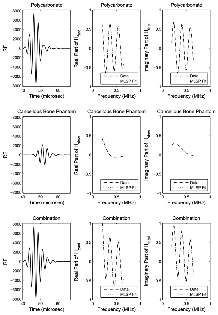
RF signals (left column), transfer functions (right column), and MLSP fits (right column) for experimental data from polycarbonate plate (top row), cancellous bone phantom (middle row), and composite signal (bottom row).

Table 1 shows a comparison of estimates of fast and slow wave attenuation slopes and phase velocities in the polycarbonate plate and in the cancellous bone phantom obtained 1) by applying the MLSP method on the combined transfer function, H_total(ω), and 2) by applying log spectral difference (Equation 4) and spectral phase velocity (Equation 5) methods on the individual transfer functions, H_fast(ω) and H_slow(ω). The MLSP method yielded estimates of attenuation slope accurate to within 7% (polycarbonate plate) and 2% (cancellous bone phantom) and estimates of phase velocity accurate to within 1.5% for both media.

Table 1.

A comparison of estimates of fast and slow wave attenuation slopes and phase velocities in the polycarbonate plate and in the cancellous bone phantom obtained 1) by applying the MLSP method on the combined transfer function, H_total(ω), and 2) by applying log spectral difference (Equation 4) and spectral phase velocity (Equation 5) methods on the individual transfer functions, H_fast(ω) and H_slow(ω).

Material	Source Signal	Method	wave	βj (dB/cmMHz)	vj(ω0) (m/s)
Composite	Htotal(ω)	MLSP	fast slow	1.97 ± 0.18 14.48 ± 0.18	2238 ± 4 1561 ± 3
Polycarbonate Plate	Hfast(ω)	Log Spectral Difference	fast	2.11 ± 0.15	-
Polycarbonate Plate	Hfast(ω)	Spectral Phase Velocity	fast	-	2212 ± 1
Cancellous Bone Phantom	Hslow(ω)	Log Spectral Difference	slow	14.78 ± 0.17	-
Cancellous Bone Phantom	Hslow(ω)	Spectral Phase Velocity	slow	-	1538 ± 2

Figure 2 shows RF signals (left column), transfer functions (middle and right columns), and MLSP fits (middle and right columns) for simulated data for the fast wave (top row), the slow wave (middle row), and the combined signal (bottom row) with v_fast(ω₀) = 2100 m/s and SNR = 20 dB. The MLSP models agree very well with the simulated transfer functions. The lower left graph shows the combined RF signal, from which the two components are not easily separated in time domain. The lower middle and lower right graphs show the result of applying the MLSP method directly to the combined transfer function H_total(ω)—without access to the individual transfer functions H_fast(ω) and H_slow(ω).

2.

RF signals (left column), transfer functions (right column), and MLSP fits (right column) for simulated data with v_fast(ω₀) = 2100 m/s and SNR = 20 dB. The lower right graph shows the result of applying the MLSP method to the combined transfer function, H_total(ω), not merely the sum of the results of applying the MLSP method to H_fast(ω) and H_slow(ω).

Figure 3 is similar to Figure 2 except with v_fast(ω₀) = 1600 m/s and SNR = 25 dB. In this case, v_fast(ω₀) is much closer than before to v_slow(ω₀), which is 1500 m/s. Therefore, the degree of overlap in the time domain is greater (see lower left graph), and the transfer functions are more similar. These conditions make the wave separation task more challenging than the conditions for Figure 2. Nevertheless, the MLSP models agree very well with the simulated transfer functions (see lower middle and lower right graphs).

3.

RF signals (left column), transfer functions (right column), and MLSP fits (right column) for simulated data with v_fast(ω₀) = 1600 m/s and SNR = 25 dB. The lower right graph shows the result of applying the MLSP method to the combined transfer function, H_total(ω), not merely the sum of the results of applying the MLSP method to H_fast(ω) and H_slow(ω).

Figure 4 shows estimates of fast and slow wave amplitudes as functions of SNR for v_fast(ω₀) = 2100 m/s. The biases in the estimates are quite small, but the variances become substantial as SNR approaches 20 dB.

4.

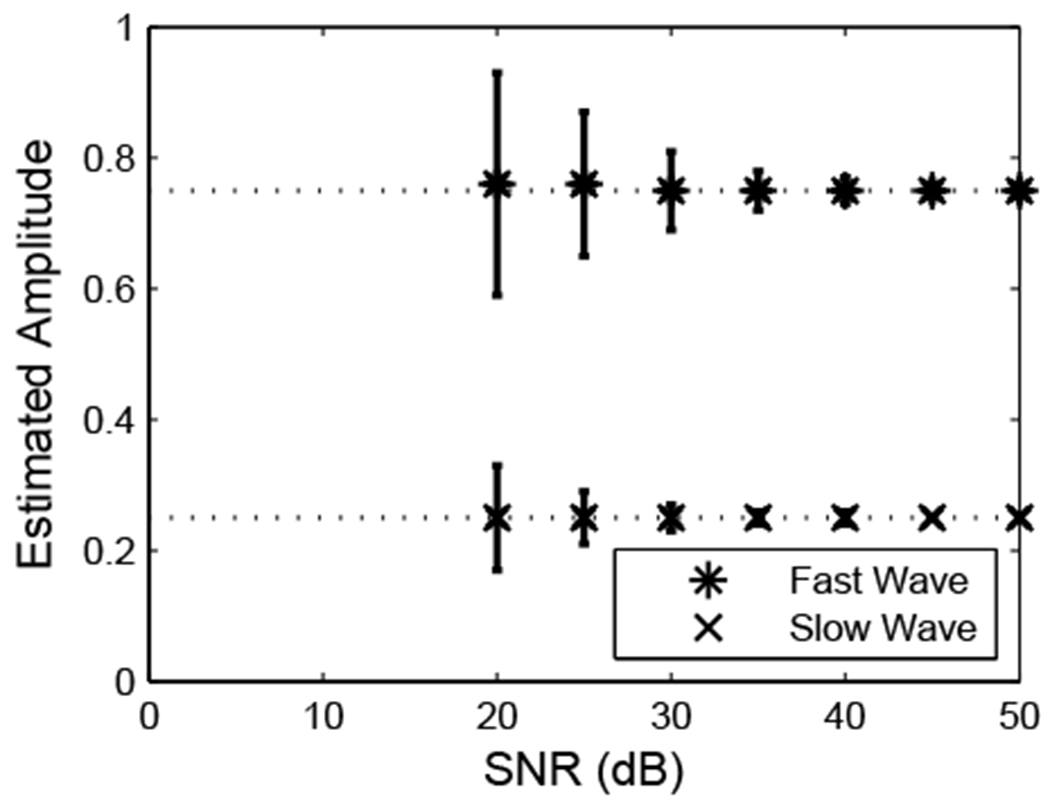
Estimates of fast and slow wave amplitudes computed using the MLSP method on the simulated data for v_fast(ω₀) = 2100 m/s.

Figure 5 shows estimates of fast and slow wave attenuation slopes as functions of SNR for v_fast(ω₀) = 2100 m/s. Again, the biases in the estimates are quite small, but the variances become substantial as SNR approaches 20 dB.

5.

Estimates of fast and slow wave attenuation slopes computed using the MLSP method on the simulated data for v_fast(ω₀) = 2100 m/s.

Figures 6 and 7 show estimates of fast and slow wave phase velocities at 1 MHz as functions of SNR for v_fast(ω₀) = 2100 m/s. The phase velocities have biases of about 90 m/s (fast wave) and 20 m/s (slow wave). These biases may be due to the assumption of zero dispersion inherent in the MLSP algorithm.

6.

Estimate of fast wave phase velocity computed using the MLSP method on the simulated data for v_fast(ω₀) = 2100 m/s.

7.

Estimate of slow wave phase velocity computed using the MLSP method on the simulated data for v_fast(ω₀) = 2100 m/s.

Figure 8 shows optimal model order as a function of SNR. Optimal model order decreases with SNR. This is reasonable because additional terms in the Prony model are required at lower SNR in order to accommodate higher noise levels.

8.

Optimum model order as a function of SNR for the simulated data for v_fast(ω₀) = 2100 m/s.

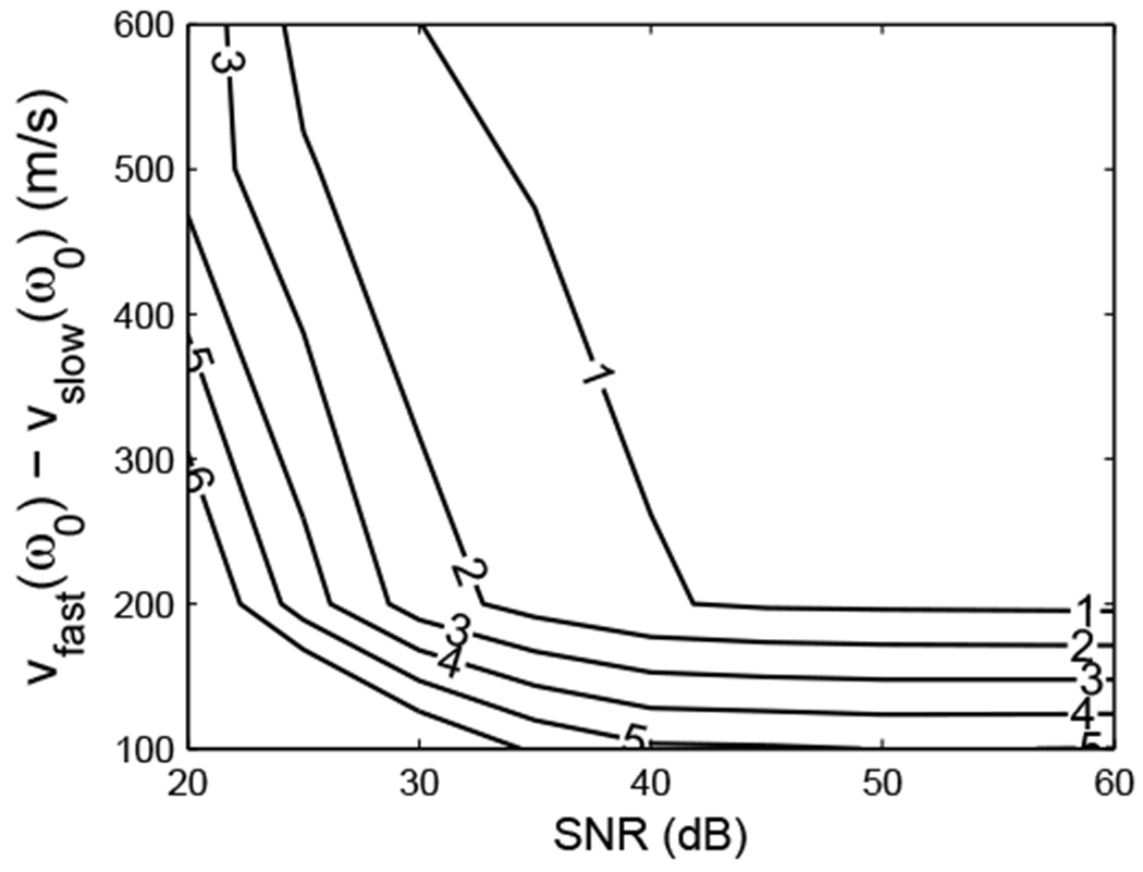
Figures 9 and 10 show contour plots of root mean square error (RMSE) in the estimates of fast (Figure 9) and slow (Figure 10) wave attenuation slopes as functions of SNR and velocity difference v_fast(ω₀) - v_slow(ω₀). Clearly, the RMSE’s of estimates decrease as SNR and velocity difference increase. The increased density of contour lines for velocity differences below 100 m/s suggests that the separation task becomes considerably more challenging when the fast and slow wave velocities approach each other.

9.

Contour plot of RMSE of the estimates of fast wave attenuation slope (dB/cmMHz) as a function of SNR and velocity difference v_fast(ω₀) - v_slow(ω₀).

10.

Contour plot of RMSE of the estimates of slow wave attenuation slope (dB/cmMHz) as a function of SNR and velocity difference v_fast(ω₀) - v_slow(ω₀).

Figures 11 and 12 show contour plots of RMSE in the estimates of fast (Figure 11) and slow (Figure 12) wave velocities as functions of SNR and velocity difference v_fast(ω₀) - v_slow(ω₀).

11.

Contour plot of RMSE of the estimates of fast wave velocity (m/s) as a function of SNR and velocity difference v_fast(ω₀) - v_slow(ω₀).

12.

Contour plot of RMSE of the estimates of slow wave velocity (m/s) as a function of SNR and velocity difference v_fast(ω₀) - v_slow(ω₀).

DISCUSSION

Pulses transmitted through cancellous bone samples contain important information regarding material and structural properties. This information can be enhanced when pulses are decomposed into fast and slow wave components. This decomposition is often challenging, however, due to temporal overlap between the two components. In this paper, the MLSP method has been shown to be effective for separating fast and slow wave components from composite pulses.

The MLSP method produces an estimate of phase velocity only at the reference frequency rather than across the entire frequency band of analysis. Full frequency-dependent phase velocity, if required, may be estimated using Equation 7 and the MLSP-based estimates of attenuation slope and phase velocities at the reference frequency (ω₀).

For values of attenuation slope and wave velocity relevant for cancellous bone samples, the MLSP method became challenged as SNR approached 25 dB or so. However, it is common to acquire laboratory data with SNR much higher than 25 dB. For example, the experimental data shown Figure 1 had an SNR of 40 dB, which is far superior to the 20 - 25 dB simulations shown in Figures 2 and 3. SNR for in vivo data is typically much lower than SNR for in vitro data. In challenging measurement conditions, SNR may be improved by averaging repeated measurements in time domain.

Decomposition of multicomponent pulses would be far more challenging in vivo (e.g., in calcaneus) than in vitro because of added signal distortion due to (1) refraction effects (primarily from cortical layers surrounding the cancellous bone), (2) beam defocusing (from phase aberration associated with tissue inhomogeneities), (3) multipath interference, (4) reverberations and (5) phase cancellation at the receiver. In addition, when the calcaneus is interrogated in the mediolateral orientation (as is the case with clinical bone sonometers), trabeculae are aligned roughly perpendicular to the beam propagation path, which results in diminished contrast in speed between fast and slow waves. Therefore, the primary application for Prony’s method (in the context of ultrasonic characterization of bone) may be to help elucidate mechanisms underlying the interaction between ultrasound and cancellous bone in experiments in vitro.

REFERENCES

- Anderson CC, Marutyan KR, Holland MR, Wear KA, and Miller JG. Interference between wave modes may contribute to the apparent negative dispersion observed in cancellous bone, J Acoust Soc Am, 2008;124:1781–1789. [DOI] [PMC free article] [PubMed] [Google Scholar]
- Bauer AQ, Marutyan KR, Holland MR, and Miller JG, Negative dispersion in bone: The role of interference in measurements of the apparent phase velocity of two temporally overlapping signals. J. Acoust. Soc. Am, 2008;123:2407–2414. [DOI] [PMC free article] [PubMed] [Google Scholar]
- Biot MA. Theory of propagation of elastic waves in a fluid saturated porous solid I. Low frequency range, J Acoust Soc Am 1956a;28:168–178. [Google Scholar]
- Biot MA. Theory of propagation of elastic waves in a fluid saturated porous solid II. High frequency range, J Acoust Soc Am 1956b;28:179–191. [Google Scholar]
- Biot MA. Theory of deformation of a porous viscoelastic anisotropic solid. J Appl Phys, 1956c;27:459–467. [Google Scholar]
- Biot MA, Generalized theory of acoustic propagation in porous dissipative media, J Acoust Soc A, 1962;34:1254–1264. [Google Scholar]
- Biot MA. Mechanics of deformation and acoustic propagation inporous media, J Appl Phys, 1963;33:1482–1498. [Google Scholar]
- Cardoso L, Teboul F, Sedel L, Oddou C, and Meunier A In vitro acoustic waves propagation in human and bovine cancellous bone, J Bone Miner Res, 2003;18:1803–1812. [DOI] [PubMed] [Google Scholar]
- Droin P, Berger G and Laugier P Velocity dispersion of acoustic waves in cancellous bone. IEEE Trans Ultrason Ferro Freq Cont 1998;45:581–592. [DOI] [PubMed] [Google Scholar]
- Fellah ZEA, Chapelon JY, Berger S, Lauriks W, and Depollier C, Ultrasonic wave propagation in human cancellous bone: Application of Biot theory, J Acoust Soc Am, 2004;116:61–73. [DOI] [PubMed] [Google Scholar]
- Fellah ZEA, Sebaa N, Fellah M, Mitri FG, Ogam E, Lauriks W, and Depollier C, Application of the Biot model to ultrasound in bone: direct problem, IEEE Trans Ultrason, Ferro, and Freq Cont, 2008;55:1508–1515. [DOI] [PubMed] [Google Scholar]
- Haïat G, Padilla F, Peyrin F, and Laugier P, Fast wave ultrasonic propagation in trabecular bone: numerical study of the influence of porosity and structural anisotropy, J Acoust Soc Am, 2008;123:1694–1705. [DOI] [PubMed] [Google Scholar]
- Haire TJ, and Langton CM. Biot Theory: A review of its application to ultrasound propagation through cancellous bone, Bone, 1999;24:291–295. [DOI] [PubMed] [Google Scholar]
- Hosokawa A and Otani T Ultrasonic wave propagation in bovine cancellous bone, J Acoust Soc Am, 1997;101:558–562. [DOI] [PubMed] [Google Scholar]
- Hosokawa A and Otani T Acoustic anisotropy in bovine cancellous bone, J Acoust Soc Am, 1998;103:2718–2722. [DOI] [PubMed] [Google Scholar]
- Hosokawa A Simulation of ultrasound propagation through bovine cancellous bone using elastic and Biot’s finite-difference time-domain methods, J Acoust Soc Am, 2005;118,:1782–1789. [DOI] [PubMed] [Google Scholar]
- Hosokawa A, Development of a numerical cancellous bone model for finite-difference time-domain simulations of ultrasound propagation, IEEE Trans Ultrason, Ferro, Freq Cont, 2008;55:1219–1233. [DOI] [PubMed] [Google Scholar]
- Hughes ER, Leighton TG, Petley GW, White PR, and Chivers RC. Estimation of critical and viscous frequencies for Biot theory in cancellous bone, Ultrasonics, 2003;41,:365–368. [DOI] [PubMed] [Google Scholar]
- Hughes ER, Leighton TG, White PR, and Petley GW, Investigation of an anisotropic tortuosity in a Biot model of ultrasonic propagation in cancellous bone, J Acoust Soc Am, 2007;121:568–574. [DOI] [PubMed] [Google Scholar]
- Kaczmarek M, Kubik J and Pakula M Short ultrasonic waves in cancellous bone, Ultrasonics, 2002;40:95–100. [DOI] [PubMed] [Google Scholar]
- Kaufman JJ, Xu W, Chiabrera AE, and Siffert RS Diffraction effects in insertion mode estimation of ultrasonic group velocity. IEEE Trans. Ultrason. Ferro., Freq. Contr, 1995;42;232–242. [Google Scholar]
- Kaufman JJ, Luo G, and Siffert RS. A portable real-time ultrasonic bone densitometer. Ultrasound Med. Biol, 2007;33:1445–1452. [DOI] [PMC free article] [PubMed] [Google Scholar]
- Kaye GWC, and Laby TH. Table of Physical and Chemical Constants. London, UK, Longman, 1973. [Google Scholar]
- Kumaresan R, and Tufts DW. Estimating the parameters of exponentially damped sinusoids and pole-zero modeling in noise, IEEE Trans. Acoust. Speech Signal Process, 1982;ASSP-30:833–840. [Google Scholar]
- Kuc R and Schwartz M. Estimating the acoustic attenuation coefficient slope for liver from reflected ultrasound signals. IEEE Trans Son Ultrason 1979;SU-26:353–362. [Google Scholar]
- Laugier P, Instrumentation for In vivo Ultrasonic Characterization of Bone Strength, IEEE Trans Ultrason Ferro, Freq Cont, 2008;55:1179–1196. [DOI] [PubMed] [Google Scholar]
- Le Floch V, McMahon DJ, Luo G, Coeh A, Kaufman JJ, Shane E, and Siffert RS. Ultrasound simulation in the distal radius using clinical high-resolution peripheral CT images. Ultrasound Med. Biol, 2008;34:1317–1326. [DOI] [PMC free article] [PubMed] [Google Scholar]
- Lee KI, Roh H, and Yoon SW. Acoustic wave propagation in bovine cancellous bone: Application of the modified Biot-Attenborough model, J Acoust Soc Am, 2003;114:2284–2293. [DOI] [PubMed] [Google Scholar]
- Lee KI, and Yoon SW. Comparison of acoustic characteristics predicted by Biot’s theory and the modified Biot-Attenborough model in cancellous bone, J Biomech, 2006;39:364–368. [DOI] [PubMed] [Google Scholar]
- Marple SL. Digital Spectral Analysis with Applications, Englewood Cliffs, NJ, Prentice-Hall Inc., 1987. [Google Scholar]
- Marutyan KR, Holland MR, and Miller JG. Anomalous negative dispersion in bone can result from the interference of fast and slow waves, J. Acoust. Soc. Am, 2006;120:EL55–EL61. [DOI] [PubMed] [Google Scholar]
- Marutyan KR, Bretthorst GL, and Miller JG. Bayesian estimation of the underlying bone properties from mixed fast and slow mode ultrasonic signals, J. Acoust. Soc. Am, 2007;121:EL8–EL15. [DOI] [PubMed] [Google Scholar]
- McKelvie ML, and Palmer SB The interaction of ultrasound with cancellous bone, Phys Med Biol, 1991;36:1331–1340. [DOI] [PubMed] [Google Scholar]
- Mizuno K, Matsukawa M, Otani T, Takada M, Mano I, and Tsujimoto T Effects of structural anisotropy of cancellous bone on speed of ultrasonic fast waves in the bovine femur, IEEE Trans Ultrason Ferro, Freq Cont, 2008;55:1480–1487. [DOI] [PubMed] [Google Scholar]
- Mohamed MM, Shaat LT, and Mahmoud AN. Propagation of ultrasonic waves through demineralized cancellous bone, IEEE Trans Ultrason, Ferro, and Freq Cont., 2003;50:279–288. [DOI] [PubMed] [Google Scholar]
- Nicholson PHF, Lowet G, Langton CM, Dequeker J, and Van der Perre G. Comparison of time-domain and frequency-domain approaches to ultrasonic velocity measurements in trabecular bone, Phys Med Biol, 1996;41:2421–2435. [DOI] [PubMed] [Google Scholar]
- Pakula M, Padilla F, Laugier P, and Kaczmarek M, Application of Biot’s theory to ultrasonic characterization of human cancellous bones: Determination of structural, material, and mechanical properties, J Acoust Soc Am, 2008;123:2415–2423. [DOI] [PubMed] [Google Scholar]
- Riekkinen O, Hakulinen MA, Timonen M, Töyräs J, and Jurvelin JS. Influence of overlying soft tissues on trabecular bone acoustic measurement at various ultrasound frequencies, Ultrasound Med. Biol, 2006;32:1073–1083. [DOI] [PubMed] [Google Scholar]
- Riekkinen O, Hakulinen MA, Töyräs J, and Jurvelin JS. Dual-frequency ultrasound—new pulse-echo technique for bone densitometry, Ultrasound Med. Biol, 2008;34:1703–1708. [DOI] [PubMed] [Google Scholar]
- Sebaa N, Fellah ZEA, Fellah M, Ogam E, Mitri FG, Depollier C, and Lauriks W Application of the Biot model to ultrasound in bone: inverse problem, IEEE Trans Ultrason, Ferro, and Freq Cont, 2008;55:1516–1523. [DOI] [PubMed] [Google Scholar]
- Strelitzki R, and Evans JA. On the measurement of the velocity of ultrasound in the os calcis using short pulses, Eur J Ultrasound, 1996;4:205–213. [Google Scholar]
- Van Blaricum ML and Mittra R A technique for extracting the poles and residues of a system directly from its transient response, IEEE Trans. Antennas Propag, 1975;AP-23:777–781. [Google Scholar]
- Waters KR and Hoffmeister BK, Kramers-Kronig analysis of attenuation and dispersion in trabecular bone, J Acoust Soc Am, 2005;118:3912–3920. [DOI] [PubMed] [Google Scholar]
- Wear KA. Measurements of phase velocity and group velocity in human calcaneus, Ultrason Med Biol, 2000;26:641–646. [DOI] [PMC free article] [PubMed] [Google Scholar]
- Wear KA, Laib A, Stuber AP, and Reynolds JC, Comparison of measurements of phase velocity in human calcaneus to Biot theory, J Acoust Soc Am, 2005;117:3319–3324. [DOI] [PMC free article] [PubMed] [Google Scholar]
- Wear KA, Group velocity, phase velocity, and dispersion in human calcaneus in vivo, J Acoust. Soc Am, 2007;121:2431–2437. [DOI] [PMC free article] [PubMed] [Google Scholar]
- Williams JL. Ultrasonic wave propagation in cancellous and cortical bone: predictions of some experimental results by Biot’s theory, J Acoust Soc Am, 1992;92:1106–1112. [DOI] [PubMed] [Google Scholar]
Associated Data
This section collects any data citations, data availability statements, or supplementary materials included in this article.