Nonlinear impact of COVID-19 on pollutions – Evidence from Wuhan, New York, Milan, Madrid, Bandra, London, Tokyo and Mexico City

Graphical abstract

Abstract

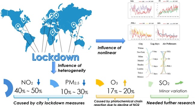
The majority of existing COVID-19 and pollution research are from a linear perspective, ignoring the nonlinear relationship between COVID-19 and pollution. This work is aimed to systematically investigate the nonlinear impact of COVID-19 lockdown on four typical pollutants (NO_2, PM2.5, O₃ and SO₂) in the selected eight cities (Wuhan of China, New York of the United States, Milan of Italy, Madrid of Spain, Bandra of India, London of United Kingdom, Tokyo of Japan and Mexico City of Mexico) using the updated data and spearman correlation function model. To a certain extent, the global lockdown caused by the coronavirus only reduces nitrogen dioxide and particles, but does not reduce ozone . Specifically, compared with the average concentration in the same period from 2017 to 2019, NO₂ in 2020 decreased by 40–50 %, PM_2.5 in 2020 decreased by 10–30 %, O₃ in 2020 increased by 17–20 % and SO₂ in 2020 increased slightly. In addition, the changes of new confirmed cases of COVID-19 and change of pollutants were not synchronized. On the contrary, there was a 0–7 days lag between the new confirmed cases and changes of pollutants.

1. Introduction

The COVID-19 has become a global pandemic, affecting more than 200 countries and territories around the world (World Health Organization, 2020). Many countries are aware that suspending public transportation, closing entertainment venues and prohibiting public gatherings are the most effective ways to stop the spread of the virus (Atalan, 2020). Of the 50 states in the United States, New York has the worst epidemic and imposed a ban on staying at home on March 22 (Ng, 2020). As the most severe country in Europe, the Italian government announced a city blockade on March 8 (Menut et al., 2020). After Italy, Spain became Europe's second closed country (March 14) (Aldaco et al., 2020). Subsequently, the British Prime Minister also announced a nationwide lockdown on March 23 (Madan, 2020). In addition to this, the Indian Prime Minister announced a nationwide curfew on March 22, canceling all domestic and international flights and other transportation. India’s four measures to extend the lockdown of the city were also of concern. The date of the closure of the city has been extended to June 30 (Sharma, Zhang, Anshika Gao, Zhang, & Kota, 2020). Following this, Mexico City and Tokyo were blocked at the end of March and early April (Masako, 2020).

The lockdown and social isolation not only shutted down some factories, but also greatly reduced the flow of traffic (Bai et al., 2020; Wang & Wang, 2020). Due to this, significant changes of air pollutions have taken place (Bashir et al., 2020; Mahato, Pal, & Ghosh, 2020). Existing studies (Chen, Kuschner, Gokhale, & Shofer, 2007; Nuvolone, Petri, & Voller, 2018) have shown that particulate matter with aerodynamic diameter less than 2.5 μm (PM_2.5), nitrogen dioxide (NO₂), sulfur dioxide (SO₂) and tropospheric ozone (O₃) are the most serious air pollutants threatening human health. Exposure to air pollutants not only threatens the human respiratory system, but can also cause potential lung diseases (Wang & Su, 2020). Taking various regions as examples to study the relationship between air pollutants and human health has always been the focus of scholars. Long-term exposure to air pollution not only promotes the spread of the virus, but also leads to high rates of respiratory and heart disease (Fattorini & Regoli, 2020). Scholars (Venter, Aunan, Chowdhury, & Lelieveld, 2020) found that in China and India alone, the number of PM_2.5 related premature deaths was 1,400 and 5,300, respectively. Older adults with comorbidities are more responsive to the environment and tend to have more severe symptoms (Wang et al., 2020).

Focused on the eight cities of Wuhan, New York, Milan, Madrid, Bandra, London, Tokyo and Mexico City, this study aims to explore the relationship between the lockdown and air pollutants (NO_2, SO_2, O_3, PM_2.5) from the perspective of nonlinearity and heterogeneity. Compared with other studies, innovations include the following two aspects. First, the moving average function and Spearman correlation function model will be used to determine the nonlinear influence of the hysteresis (0 day, 3 days, 5 days and 7 days) of newly confirmed COVID-19 cases on the changes of four environmental pollutants. Secondly, through the investigation of the urban lockdown period in 2020 and the same period from 2017 to 2019, the heterogeneous impact of each city's lockdown on its air pollutants will be investigated from the angle of intensity distribution and statistics in bubble diagram and boxplot respectively. Comparisons are made between quartiles, medians, and 95 % confidence intervals. The practice of this study aims to reveal how the lockdown caused by COVID-19 will affect the air quality of eight cities.

2. Methods

2.1. Area and indicator selection

Areas most affected by the epidemic impose more obvious significance for air quality (Zhu, Xie, Huang, & Cao, 2020). The cities of Wuhan, New York, Milan, Madrid, Bandra, London, Tokyo and Mexico City have a very high number of confirmed cases during the New Coronary Pneumonia epidemic (Onder, Rezza, & Brusaferro, 2020). More notably, these eight cities have all adopted the measures of city lockdown in response to the epidemic. Leaders of various countries have also announced specific city lockdown dates through media. Except for Wuhan's lockdown of the city on January 23, the other seven cities have all implemented lockdown in March and April (Milan on March 8, Madrid on March 14, New York on March 22, Bandra on March 25, London on March 23, Tokyo on April 7 and Mexico City on March 30).

NO₂, O₃, SO₂ and PM_2.5 are common indicators of measuring air quality (Chauhan & Singh, 2020; He, Pan, & Tanaka, 2020; Ogen, 2020). In this study, these pollutants are selected for analysis. The data source of each pollution indicator varies from country to country. Specifically: (1) New York’s air pollutants daily data period 2017–2019 was obtained from the United States Environmental Protection Agency (EPA) (Environmental Protection Agency, 2020). NO₂ (unit: ppb) is measured by daily max 1 -h NO₂ concentration; O₃ (unit: ppb) is measured by daily max 8-h O₃ concentration; SO₂ (unit: ppb) is represented by daily max 1 -h SO₂ concentration; PM_2.5 (unit: ug/m³ LC) is represented by daily mean PM_2.5 concentration. (2) The air pollutants daily data of Wuhan, New York, Milan, Madrid, Bandra, London, Tokyo and Mexico City are selected from World Air Quality Index (AQI, 2020), which has been investigating with the most relevant international institutions. This is an open data platform providing free access the world historical and real-time Air Quality data from the 100+ countries. The pollutant data of several cities derived from this database are all daily average values. The unit of each pollutant is the same as that of New York.

Considering that the impact of the epidemic on air pollutants is mainly achieved through the lockdown of the city, selected period for observation is from the beginning of the lockdown to October 30. For example, daily data for pollution indicators in Wuhan ranges from January 23 to October 30, while that of New York selected from March 22 to October 30. Comparing the content of pollutants in 2020 and the historical period is the key to analyze the impact of the epidemic on air pollutants. To set up a control groups, all air quality indicators during observation date in 2017–2019 years were used for obversion. Obtained comparison results could uncover the true relationship and influence between the lockdown and air pollutants.

2.2. Data processing by box-plot

Box plot is a statistical chart used to display the distribution pattern of a set of dispersion data. On the one hand, it can reflect the characteristics of the original data distribution; on the other hand, it can compare the distribution characteristics of multiple sets of data. Generally speaking, a box plot consists of the upper edge, lower edge, median, and two quartiles of a set of data (Hintze & Nelson, 1998). A more specific box plot will also indicate the data range within the 95 % confidence interval. The drawing of the box plot does not impose any restrictive requirements. This method relies on actual data and does not require that the data follow a specific distribution form in advance (Williamson, Parker, & Kendrick, 1989). Therefore, this is a statistical analysis method that can truly and intuitively express the original appearance of the data shape.

In practice, the quartile value is the key calculated point. The upper and lower quartiles are usually represented by Q₁ and Q₃ (calculated following equation $Q_i=\frac{n-1}{4}$). In the determination process, the data needs to be rearranged according to the size of the value (Mirzargar, Whitaker, & Kirby, 2014). The data at Q₁ and Q₃ represent the lower quartile and upper quartile, respectively. The quartile has a certain stability, as much as 25 % of the data can be arbitrarily varied without greatly disturbing the quartile. Therefore, the outliers cannot exert influence on this standard (Dawson, 2011), which makes the result of identifying abnormal values in the box plot more objective (Large, Gemmell, Paulick, & Huston, 2001).

In addition to quartiles, the median is also the key drawn point in the box plot. Median refers to the data in the middle of a series of data. Besides, the distribution of data within the 95 % confidence interval is also the focus of describing statistical characteristics. The data in this interval can often represent the distribution of the array. This has become an important reference standard other than quartiles. On the same number axis, box plots of each group of data are arranged in parallel. Shape information such as the median, tail length, outliers, and distribution interval of several batches of data is clear at a glance. This will provide a simple and direct way to compare and analyze the differences between the data of each group.

2.3. Spearman correlation function model

Spearman correlation coefficient, also commonly called Spearman rank correlation coefficient (Croux & Dehon, 2010). Rank can be understood as a sort or order, then it is solved according to the sort position of the original data. It abandons the traditional Pearson method's requirement for data, that is, the data must be in a normal distribution and linearly related. Since the rank of outliers usually does not change significantly (for example, if it is too large or too small, it will be ranked first or last) (Bonett & Wright, 2000), so the influence on Spearman's correlation coefficient is also very small. This has become the advantage of this correlation coefficient calculation method.

The calculation of the correlation coefficient follows the following steps.

Step 1: Define two sets of data sequences: $\text{X}=\left\{x_1,x_2,\cdots ,x_n\right\}$ and $\text{Y}=\left\{y_1,y_2,\cdots ,y_n\right\}$. Sort the data by size, and define the sorted data sequence as $X^{\text{'}}=\left\{x_i^{\text{'}},x_i^{\text{'}},\cdots ,x_i^{\text{'}}\right\}$ and $Y^{\text{'}}=\left\{y_i^{\text{'}},y_i^{\text{'}},\cdots ,y_i^{\text{'}}\right\}$.

Step 2: Rank as the position of the $x_i$ in the $X^{\text{'}}$ sequence, and the position of the $y_i$ in the $Y^{\text{'}}$ sequence and record the rank of $\left[\left(x_1,y_1\right),\left(x_2,y_2\right),\cdots \left(x_n,y_n\right)\right]$ as $\left[\left(T_1,S_1\right),\left(T_2,S_2\right),\cdots \left(T_n,S_n\right)\right]$.

Step 3: Calculate the estimated value of the overall correlation coefficient “R”:

$$\text{R}=1-\frac{6\sum _{i=1}^n{\left(T_i-S_i\right)}^2}{n(n^2-1)}$$

Step 4: Perform a two-tailed significance test on the obtained significance results to compare whether ‘A ’ and ‘B’ are significantly different. When p < 0.05, it is considered statistically significant (Myers & Sirois, 2006).

3. Hysteresis effects of COVID-19 on air pollutants

To verify the correlation between the COVID-19 and air quality, the correlation between new coronavirus infection cases and air pollutants emissions will be tested through Spearman correlation function model. In addition, the daily content of pollutants in 2020 will be compared with the daily averaged content in 2017–2019. These yearly comparison helps to measure the overall air quality under the epidemic.

3.1. Pollutant emission curve in 2020 and 2017–2019

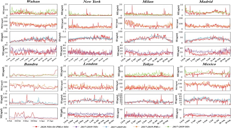
With reference to the database mentioned above, Fig. 1 plots the time-series trend of four pollutants period 2017–2020. We set the pollutant emissions in 2020 as observation sample and the averaged pollutant emissions from 2017 to 2019 as control sample. As we all know, the emission of air pollutants is affected by many factors. In this case, choosing the air pollution data of the past three years as the comparison for 2020 can basically eliminate the impact of specific years/events on the current pollutants. In below figure, the red line represents the emissions of various pollutants from January 1, 2020 to October 30, 2020. The other colored lines in Fig. 1 mean the historical averaged level of air pollutants from January 1 to October 30 over the 2017–2019.

Fig. 1.

Comparison chart of 2017–2019 and 2020 in four pollutants.

According to existed studies, the amount of pollutants in the air will be affected by weather and other factors (Pei, Han, Ma, Su, & Gong, 2020). When pollutants enter the lower atmosphere through pollution sources, they flow downstream with the dominant wind direction on the one hand and diffuse around with atmospheric turbulence on the other hand (Higham, Green, & Ramirez, 2020). Therefore, pollutants in the atmosphere are closely related to wind, temperature inversion, diffusion conditions and other meteorological factors. In order to eliminate the interference of exclusion factors, we set the date of the observation sample and the control sample to the comparison of daily emissions in the same time period. According to the latest data source provided by the database, the content of each pollutant during the period from January 1 to October 30 was selected and plotted as shown in Fig. 1. First, the graph plots the NO₂ air content in eight cities. The curve shows that compared with 2017–2019 (purple line), the NO₂ level in 2020 (red line) is lower. Through further comparison, this phenomenon is more obvious in 6 cities except Bandra and Tokyo. Secondly, the chart compares the dynamic trends of O₃ in 2020 (red line) and 2017–2019 (blue line). Many cities show that the ozone content is not much different from previous years. In addition, there are also significant differences in the annual emissions of PM2.5 and SO₂ between 2017–2019 and 2020 (both pollutants show that emissions in 2020 are lower than in previous years). Based on the above points, we can conclude that: In the observed city, the amount of pollutant emissions in 2020 show varying degrees of change from historical levels. The specific link between pollutants and urban blockades needs further study.

3.2. Correlation between confirmed cases and pollutants

Since the outbreak of Corona Virus Disease, the number of confirmed cases is increasing every day. The confirmed number of cases per day has become an indicator judging the severity of the epidemic. We input the number of confirmed cases and air pollutants on one day into the correlation test model. Notably, considering that there is a lag in the response of the society to the epidemic, the data was processed with a lag of five days before the correlation was measured. Calculated correlation coefficients could quantify the relationship between the two.

Table 1 lists the correlation coefficient between the number of illnesses and pollutants in each city. It can be seen that NO₂ is negatively correlated with the number of COVID-19 cases in eight cities. In addition, the emissions of SO₂ and PM_2.5 are negatively correlated with cases of Corona Virus Disease in five cities. The relationship between O₃ and the epidemic are positively correlated in five cities. It can be seen from this that, regardless of the number of lag days, the correlation between NO₂ and the epidemic is consistent in all cities. However, O₃, PM_2.5 and SO₂ are consistent in part of cities. In other words, the reasons for the difference between cities are related to the consideration of the number of lag days.

Table 1.

Correlation between COVID-19 and air pollutants.

Note: ** indicates that the correlation is significant at the 0.01 level (two-tailed).

* indicates that the correlation is significant at the 0.05 level (two-tailed).

The strength of the correlation between the Corona Virus Disease epidemic and pollutants is mainly achieved through response measures. Judging from the significant level of related impact, the number of confirmed cases in Madrid has a significant impact on all four pollutants. Bandra, London and Tokyo have a significant impact on the three pollutants. New York, Milan and Mexico have significant effects on the two pollutants. The impact of confirmed cases in New York on pollutants is not significant.

3.3. Hysteresis effects of confirmed cases on pollutants

The delayed response of air pollutants to the epidemic determines that the impact of city blockade on pollutants tends to be non-linear. In fact, environmental pollutants do not necessarily change immediately after the outbreak of the Corona Virus Disease. The correlation between the epidemic and pollutants usually reaches its maximum after 0–7 days. To find out how many lag days behind the pollutants are the most relevant to the Corona Virus Disease, this section uses the moving mean function and spearman correlation function model to calculate the statistical significance and influence coefficient of the new cases of Lag 0, Lag 3, Lag 5, and Lag 7 on the four pollutants.

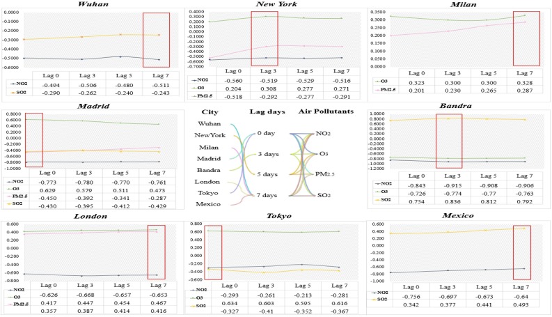
In Fig. 2 , pollutants that have significant correlation with each city are listed in the form of influence coefficient curves under different lag days. Only the correlation indicators that have passed the standard inspection are shown. The abscissa in the curve is 0 days, 3 days, 5 days and 7 days lag, and the ordinate represents the correlation coefficient value. It can be seen from the ordinate of the curve that the correlation coefficient has positive and negative numbers. When the correlation coefficient is positive, the larger the value, the stronger the correlation; when the correlation coefficient is negative, the smaller the value, the stronger the correlation.

Fig. 2.

Hysteresis of COVID-19 and environmental pollutants.

On the one hand, we find the lag days corresponding to the maximum correlation coefficient to figure out the best response time of each city to the Corona Virus Disease. The most intuitive thing from the whole, the correlation between pollutants and coronavirus disease reaches its maximum after a certain number of lag days. The number of lag days in different cities is heterogeneous. For Wuhan, London and Mexico, new cases with a lag of 7 days had the greatest impact coefficient on pollutants. During the epidemic, there is a 7-day lag in the change of pollutants in Wuhan. For New York, the effect of new cases on pollutants was greatest at a 3-day lag, compared with a 0-day lag of 5 and 7 days. During the epidemic, there is a 3-day lag in the change of pollutants in New York. For Milan, new cases with a lag of 7 days had the greatest impact on the pollutant. That is to say, during the pandemic, there was a seven-day lag in the change of pollutants in the city of Milan. For Bandra, new cases with a lag of 3 days had the greatest impact coefficient: -0.915 in NO₂, -0.774 in O₃, 0.836 in SO₂. These three coefficients are larger than the absolute values of the coefficients for the remaining 0, 5, 7 lag days. So, we have reason to believe that there is a 3-day lag in the change of pollutants in the city of Bandra during the outbreak. Only Madrid and Tokyo had a response time of zero days to COVID-19. This means that Madrid's air pollutants did not lag the outbreak.

On the other hand, the types of pollutants related to each city are different. Among the pollutants to be studied, only the number of cases in Madrid is related to the four pollutants. The new crown epidemic in the remaining cities is only related to 2–3 pollutants. Specifically, the epidemic in Wuhan and Mexico has a significant impact on NO₂ and SO₂. Milan has a significant influence on PM_2.5 and O₃ changes. NO₂, O₃, and PM_2.5 reflect the epidemic situation in New York and London. NO₂, O₃ and SO₂ were significantly affected by Bandra and Tokyo. Madrid had a significant effect on all four selected pollutants.

The above analysis illustrates the fact that the impact of the epidemic on pollutants is often non-linear. For most cities, pollutants usually change after a few days after the outbreak. Different cities have different lag days. Judging from the lag effect of pollutants after the outbreak, the lag days of pollutant changes in Wuhan, Milan, London and Mexico are both 7 days, and the reaction time is the longest. The lag days in New York and Bandra are both 3 days, and the reaction time is centered. The response of the pollutants in Madrid and Tokyo is more immediate.

4. Heterogeneous effects of lockdown on air pollutants

Taking the start date of the lockdown to October 30 as the sample interval, the analysis of four types of pollutant emissions in eight cities from 2017 to 2020 will be analyzed and discussed in this chapter. Among the selected years, 2020 is the observation year, and 2017–2019 is the control year. The reason for choosing the three years 2017–2019 for comparison is to reduce the impact of the particularity of a single historical year. By comparing the pollutant content in 2020 with the pollutant content in 2017, 2018 and 2019, we can clearly understand the macroscopic impact of urban lockdown on pollutants.

The display of the bubble diagram and box plot will be displayed at the same time. It is important to distinguish the different functions of the two forms of graphs. The bubble diagram is only a macro view of the overall emission of pollutants over the years. The boxplot is a statistical analysis of the process of the specific numerical analysis. In this part of the content, Section 4.1 will analyze the bubble chart of pollutants of eight cities one by one. Sections 4.2–4.5 respectively introduce the statistical variables of the four pollutants in each city. These will help to visually compare the inter-city changes of pollutants.

4.1. Pollutant intensity in eight typical cities

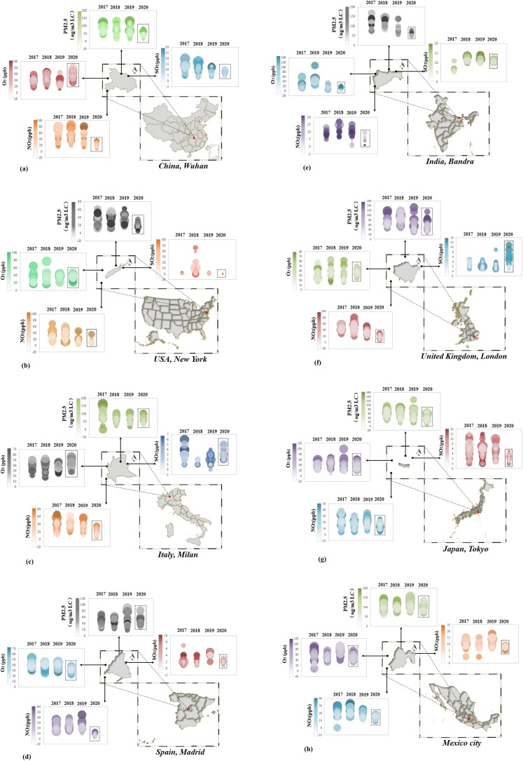
Fig. 3(a–h) shows the emission intensity of four pollutants in eight typical cities in the form of bubble diagram. On the one hand, the location of the bubble diagram represents the size of the pollutant content. On the other hand, the depth of bubble color represents the density at this content. Some findings in the emission intensity of each city since 2017 are revealed.

Fig. 3.

(a). Comparison chart of Wuhan in four pollutants. (b). Comparison chart of New York in four pollutants. (c). Comparison chart of Milan in four pollutants. (d). Comparison chart of Madrid in four pollutants. (e). Comparison chart of Bandra in four pollutants. (f). Comparison chart of London in four pollutants. (g). Comparison chart of Tokyo in four pollutants. (h). Comparison chart of Mexico city in four pollutants.

The first is the comparison of the intensity of pollutants in Wuhan (as shown in Figure (a)). The emission charts of four pollutants in Wuhan are shown in yellow, red, green and blue. After comparison with previous years, NO₂, PM_2.5 and SO₂ showed significant decreases in the observation period in 2020. The decline of NO₂ is more obvious. The pollutant rising during the observation period is O₃. In New York City, NO₂, O₃, PM_2.5 and SO₂ are shown in yellow, green, black and red. As can be seen from the figure, only the intensity of NO₂ and PM_2.5 showed sudden changes in 2020, and both presented a downward trend. The other two pollutants did not differ significantly by 2020 (as shown in Figure (b)). In Milan, the two most variable pollutants are NO₂ and O₃. Where, the strength of NO₂ decreases while that of O₃ increases. Although SO₂ is also different from previous years, the degree of change is not obvious (as shown in Figure (c)). In Madrid, there were significant decreases in NO₂ and O₃ in 2020. The decrease of NO₂ is more drastic than that of O₃. There was no significant change in PM_2.5 and SO₂ (as shown in Figure (d)). In Bandra, NO₂, O₃ and PM_2.5 showed a significant decrease in 2020, while SO₂ showed no difference from previous years (as shown in Figure (e)). In London, the concentrations of NO₂, O₃ and PM_2.5 have all declined significantly in 2020. Although the concentration of SO₂ has increased, the absolute increase is small (as shown in Figure (f)). In Tokyo, the emissions of the four pollutants in 2020 have all reduced to varying degrees. Compared with historical years, the decline of NO₂ and SO₂ is the most obvious, while that of O₃ and PM_2.5 is relatively slight (as shown in Figure (g)). In Mexico City, the content of NO₂ and SO₂ has shown a significant decline in 2020. The changes in O₃ and PM_2.5 in 2020 are not obvious from a macro perspective (as shown in Figure (h)).

Bubble diagrams show only general differences, and the exact magnitude needs to be calculated statistically. According to the above analysis, NO₂ showed a uniform decline in 2020 in all the eight cities. The decline was widespread in the selected cities. In addition, PM_2.5 intensity dropped significantly in the five cities. It's worth noting that, there was little change in SO₂ in almost all the cities observed. The variation of O₃ intensity in 2020 is unstable. Three cities went down, four cities went up. Further analysis is needed.

4.2. Nitrogen dioxide

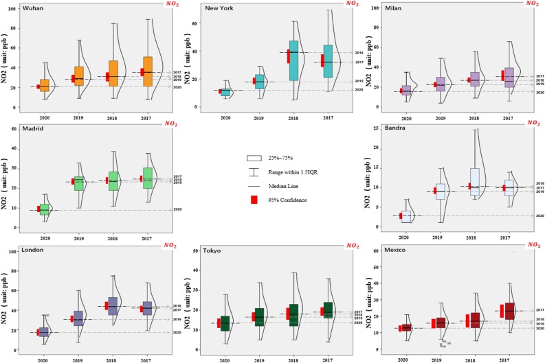
Nitrogen dioxide (NO₂) floating in the atmosphere can cause acid rain and respiratory infections. This study selected the NO₂ content in the air of eight major cities since its lockdown in 2020 as observation samples. In addition, NO₂ from the same date and in 2017–2019 years were also used as a control group. From the analysis given in Fig. 4 , The quartile range, median range of NO₂ emissions in each city and year are clearly displayed. To judge scientifically, this study uses the upper and lower values of the data distribution within the 95 % confidence interval as the standard for comparison.

Fig. 4.

Daily average concentration of NO₂ during 2017–2020 periods.

The average concentrations of NO₂ in Wuhan from 2017 to 2019 are 38 ppb, 36 ppb, 34 ppb, respectively. And in 2020 this value changes to 22 ppb, with the drop rate of 35 %–42 %. Like Wuhan, other cities all experienced significant declines in 2020 during the observation period. Specifically, Bandra has the highest NO₂ decline (70%–72%), followed by Madrid (61%–64%). London's NO₂ content was 42 ppb, 44 ppb, and 31.5 ppb in the order of 2017–2019, and it plummeted in 2020, reaching 17.8 ppb (45%–61%). The pollutants in New York fell from 19 ppb in 2019 to 12 ppb in 2020, with a decline of 37 %. Milan and Mexico City's NO₂ change rate are second only to New York, with 30 %–43 % and 18%–46% respectively. Tokyo has the smallest decline, at 23%–32%. From this data analysis, the NO₂ emissions of all cities have decreased during the lockdown period.

NO₂ produced by human activities are mostly concentrated in cities, industrial areas and densely populated areas (Zoran, Savastru, Dan, & Tautan, 2020). According to existing research statistics (Maria Cristina Collivignarelli et al., 2020), the amounts produced by high-temperature fuel combustion and city car exhaust accounts for more than 90%, and the remaining 10% mainly comes from chemical production (Otmani, Benchrif, Tahri, Bounakhla, & Krombi, 2020). For all eight cities, the reason for the consistent decline in NO₂ is related to both. On the one hand, the lockdown has greatly reduced the frequency of motor vehicle travel. The reduction of exhaust gas plays a vital role in the reduction of NO₂. On the other hand, some factories were closed during the lockdown, which also curbed production of NO₂.

Of all the cities, Bandra saw the largest decline. The reason for this phenomenon is closely related to the historical pollution performance of this city. Mumbai, to which Bandera belongs, is shrouded in haze all year round and is one of the most polluted cities in the world. Since the lockdown began on March 25, all factories, shops and religious sites have been closed, public transportation and construction activities have been suspended, and people across the country have been asked to stay at home and maintain social distance. This kind of high-strength blockade measures has made a lot of efforts for the improvement of air quality. This resulted in significant differences in NO₂ content compared with the historical period. Madrid has also seen significant declines due to historical pollution. In the past few years, Madrid has repeatedly used the Agreement on High Nitrogen Dioxide Pollution and has even been sued by the European Union for excessive NO₂ pollution. Except for these two cities, the concentration of nitrogen dioxide in the remaining cities has shown a general decline of 30%–40%, which is a normal level caused by the lockdown.

4.3. Particulate matter

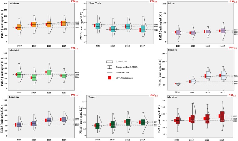
Particulate matter refers to particles with an aerodynamic equivalent diameter of 2.5 microns or less in ambient air. It can be suspended in the air for a long time. The higher the concentration in the air, the more serious the air pollution (Yao et al., 2002). Fig. 5 compares the content of PM_2.5 in the air during the observation period in various cities. Wuhan, Milan, Bandra, London, Tokyo and Mexico City all experienced a drop in PM_2.5 concentration during the 2020. However, the PM_2.5 concentration in two cities (New York and Madrid) in 2020 did not show anomalies with the past.

Fig. 5.

Daily average concentration of PM_2.5 during 2017–2020 periods.

Specifically, among the six cities that experienced a decline in PM_2.5 during the lockdown, Bandra had the largest decline, followed by London, Wuhan and Tokyo. The decline rate in these three cities ranges from 10% to 32%. Bandra fell from 75 μg/m in 2019 to 58 μg/m in 2020. The content of PM_2.5 in London fell from 50 μg/m in 2019 to 45 μg/m in 2020. Wuhan fell from 135 μg/m in 2019 to 114 μg/m in 2020. The rate of decline in Tokyo is a minimum of 12% to a maximum of 27%. Although the PM_2.5 in Milan and Mexico City have fallen from previous years, the decline is not significant enough. The reduction in PM_2.5 is inextricably linked to the traffic control imposed by the lockdown (Chauhan & Singh, 2020). In fact, the lockdown of the city limits local traffic and the burning of building fuel, which inhibits the production of PM_2.5. In addition, it is worth noting that the nitrogen oxide emissions of these cities have decreased significantly, which also restricts the indirect conversion of nitrogen oxides to PM_2.5.

For New York and Madrid, the PM_2.5 content during the closure period is basically the same as that of 2017–2019. This phenomenon in the New York area has a necessary relationship with the rebound of sulfides during the closure of the city. And for Madrid, the PM_2.5 reduction caused by the closure of the city is offset by the increase in PM_2.5 generated by family activities (such as home heating and biomass burning).

4.4. Ozone

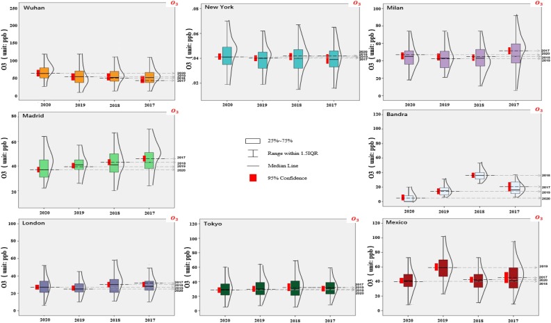
O₃ is a colorless gas with a special smell. In the near-surface layer, O₃ is produced by automobile exhaust, forest fires, volcanic eruptions, and nuclear explosions. Fig. 6 plots the O₃ emissions of the eight cities during the lockdown. In the sample surveyed, O₃ levels in the five cities in 2020 were not significantly different from those in 2017–2019. In a few cities, the O₃ content appears to increase.

Fig. 6.

Daily average concentration of O₃ during 2017–2020 periods.

Wuhan is the city that has seen an upward trend during the survey period. In Wuhan, O₃ underwent a 17 % ascent rate compared to 2017–2019. During the epidemic, the O₃ concentration increased is not a new discovery in the academic world. Existed studies have confirmed that, part of the O₃ emission is related to the concentration of NO₂ (Sicard, Marco, Agathokleous, Feng, & Calatayud, 2020). As a photochemical product, due to the non-linear characteristics of the ‘chain reaction’ of photochemical reactions, the O₃ concentration will often be opposite to the changes in nitrogen oxide emissions. Specifically, nitrogen oxides have the effect of consuming free radicals. When the concentration of nitrogen oxides in the air drops, free radicals in the atmosphere are forced to react with other contents, and under the action of photochemical reactions, the production of ozone is increased. Thus, the decrease in the content of NO₂ in the air will increase the titer of O₃ in the air. Due to the reduction of local NO₂ by road transportation, the titer of O₃ in the atmosphere is also reduced (Li et al., 2017). This became the main reason for the increase in O₃ content during the lockdown period.

Overall, it remained constant concentration in London, Milan, New York, Mexico and Tokyo. In the other samples surveyed, O₃ levels have decreased significantly. In fact, a 10% drop rate appears in Madrid (from 42 ppm in the 2019 period to 38 ppm in the 2020 period). According to some investigations, the lockdown period has increased the intensity of home activities. O₃ emissions from household and garden activities are the main reason.

4.5. Sulfur dioxide

Sulfur dioxide (SO₂), as one of the main pollutants in the atmosphere, is the most common, simple, and irritating gas (Savard, Bégin, & Parent, 2002). Sources of SO₂ pollution include the combustion of coal and petroleum, the discharge of hydrogen sulfide in oil and gas well operations, and production processes such as chemical, oil refining, and sulfuric acid plants (Otmani et al., 2020). Due to the single source of production, the atmospheric content of SO₂ is the least relative to several other pollutants (Nirel & Dayan, 2001). It is for this reason that there was no significant fluctuation in atmospheric SO₂ emissions during the closure of the city (compared to the same period in history).

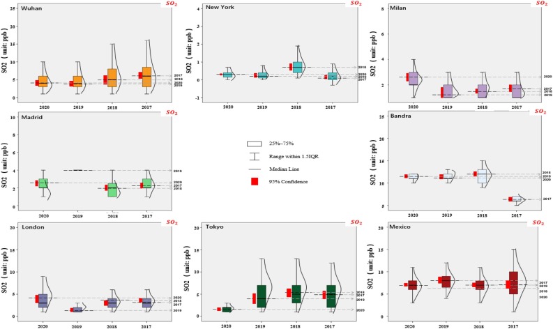
Fig. 7 shows the SO₂ content in eight cities during the observation period. Except for Wuhan, London, Milan and Tokyo, the SO₂ content of the remaining five cities are stable with the historical content value, indicating that SO₂ has not been affected by the closure of the city. Tokyo and Wuhan have a significant decline in SO₂ content in 2020, with a decrease of 57%–63% and 6%–33% respectively. Sulfur dioxide in London and Milan increased slightly. The cause of this situation may be related to continuous heating. To cope with the cold, the heating equipment in some cities has not been shut down due to the lockdown of the city. This also makes the SO₂ emissions caused by fuel combustion basically the same as in previous years.

Fig. 7.

Daily average concentration of SO₂ during 2017–2020 periods.

5. Conclusion

The outbreak of the new coronavirus has forced major cities around the world to adopt lockdown measures to respond, which indirectly affected the content of air pollutants. Through the historical data survey of eight cities and four air pollutants, two following findings were made.

First, the city lockdown had a non-linear impact on air pollutants, specifically manifested in hysteresis. Air pollutants in different cities usually different lag days after an outbreak occurs. By comparing the maximum correlation coefficient, the response time of pollutants in Wuhan, Milan, London and Mexico to the pandemic was seven days, with the longest response time. In Both New York City and Bandra, there were 3 lag days, with middle response time. The response time of pollutants in Madrid and Tokyo was more immediate. Second, the impact of the lockdown on different pollutants was heterogeneous, rather than a single increase or decrease. From the general law, NO₂ showed the largest decline during 2020 lockdown, followed by PM_2.5. O₃ was inclined to increase at a slow rate, because of the photochemical chain reaction caused by the decline of NO₂. The change of SO₂ was the least obvious among four pollutants.

The investigation of this study had enriched the link between the Corona Virus Disease and pollutants. It clearly demonstrated that the reduction of traffic volume would significantly reduce the emissions of NO₂ and PM_2.5. To a certain extent, the lockdown caused by the coronavirus only reduces nitrogen dioxide and particles but does not solve the ozone problem. In the absence of other stimuli, O₃ would indirectly affected and increases in this process. This suggested that reducing traffic pollution and limiting other anthropogenic activities were the most effective way to help improve air quality. At the same time, additional work needs to be done to reduce O₃ and SO₂.

Declaration of Competing Interest

The authors declare that they have no known competing financial interests or personal relationships that could have appeared to influence the work reported in this paper.

References

- Aldaco R., Hoehn D., Laso J., Margallo M., Salmón R., Cristobal J.…Bayer B. Environmental and nutritional impacts of dietary changes in Spain during the COVID-19 lockdown. Ence of the Total Environment. 2020 doi: 10.1016/j.scitotenv.2020.141410. [DOI] [PMC free article] [PubMed] [Google Scholar]
- AQI . 2020. Air quality historical data platform.https://aqicn.org/data-platform/register/ Retrieved from. [Google Scholar]
- Atalan A. Is the lockdown important to prevent the COVID-19 pandemic? Effects on psychology, environment and economy-perspective. Annals of Medicine and Surgery. 2020;56:38–42. doi: 10.1016/j.amsu.2020.06.010. [DOI] [PMC free article] [PubMed] [Google Scholar]
- Bai Y., Yao L., Wei T., Tian F., Jin D.-Y., Chen L.…Wang M. Presumed asymptomatic carrier transmission of COVID-19. JAMA. 2020;323(14):1406–1407. doi: 10.1001/jama.2020.2565. [DOI] [PMC free article] [PubMed] [Google Scholar]
- Bashir M.F., Ma B., Bilal Komal B., Bashir M.A., Tan D., Bashir M. Correlation between climate indicators and COVID-19 pandemic in New York, USA. The Science of the Total Environment. 2020;728 doi: 10.1016/j.scitotenv.2020.138835. [DOI] [PMC free article] [PubMed] [Google Scholar]
- Bonett D.G., Wright T.A. Sample size requirements for estimating pearson, kendall and spearman correlations. Psychometrika. 2000;65(1):23–28. doi: 10.1007/BF02294183. [DOI] [Google Scholar]
- Chauhan A., Singh R.P. Decline in PM2.5 concentrations over major cities around the world associated with COVID-19. Environmental Research. 2020;187 doi: 10.1016/j.envres.2020.109634. [DOI] [PMC free article] [PubMed] [Google Scholar]
- Chen T.-M., Kuschner W.G., Gokhale J., Shofer S. Outdoor air pollution: Nitrogen dioxide, sulfur dioxide, and carbon monoxide health effects. The American Journal of the Medical Sciences. 2007;333(4):249–256. doi: 10.1097/MAJ.0b013e31803b900f. [DOI] [PubMed] [Google Scholar]
- Croux C., Dehon C. Influence functions of the Spearman and Kendall correlation measures. Statistical Methods & Applications. 2010;19(4):497–515. doi: 10.1007/s10260-010-0142-z. [DOI] [Google Scholar]
- Dawson R. How significant is a Boxplot Outlier? Journal of Statistics Education. 2011;19(2) doi: 10.1080/10691898.2011.11889610. null-null. [DOI] [Google Scholar]
- Environmental Protection Agency . 2020. Outdoor air quality data.https://www.epa.gov/outdoor-air-quality-data/download-daily-data Retrieved from. [Google Scholar]
- Fattorini D., Regoli F. Role of the chronic air pollution levels in the Covid-19 outbreak risk in Italy. Environmental Pollution. 2020;264 doi: 10.1016/j.envpol.2020.114732. [DOI] [PMC free article] [PubMed] [Google Scholar]
- He G., Pan Y., Tanaka T. medRxiv; 2020. COVID-19, city lockdowns, and air pollution: Evidence from China. 2020.2003.2029.20046649. [DOI] [Google Scholar]
- Higham J.E., Green M.A., Ramirez C.A. 2020. UK COVID-19 Lockdown: What are the impacts on air pollution. [Google Scholar]
- Hintze J.L., Nelson R.D. Violin plots: A Box plot-density trace synergism. The American Statistician. 1998;52(2):181–184. doi: 10.1080/00031305.1998.10480559. [DOI] [Google Scholar]
- Large R.R., Gemmell J.B., Paulick H., Huston D.L. The alteration Box plot: A simple approach to understanding the relationship between alteration mineralogy and lithogeochemistry associated with volcanic-hosted massive sulfide deposits. Economic Geology. 2001;96(5):957–971. doi: 10.2113/gsecongeo.96.5.957. [DOI] [Google Scholar]
- Li G., Bei N., Cao J., Wu J., Long X., Feng T.…Tie X. Widespread and persistent ozone pollution in eastern China during the non-winter season of 2015: observations and source attributions. Atmospheric Chemistry and Physics. 2017;17(4):1–39. [Google Scholar]
- Madan V. Resumption of laser/IPL skin services post COVID-19 lockdown—British Medical Laser Association (BMLA) guidance document. Lasers in Medical Ence. 2020;(5):1–5. doi: 10.1007/s10103-020-03086-z. [DOI] [PMC free article] [PubMed] [Google Scholar]
- Mahato S., Pal S., Ghosh K.G. Effect of lockdown amid COVID-19 pandemic on air quality of the megacity Delhi, India. The Science of the Total Environment. 2020;730 doi: 10.1016/j.scitotenv.2020.139086. [DOI] [PMC free article] [PubMed] [Google Scholar]
- Maria Cristina Collivignarelli A., Abbà A., Bertanza G., Pedrazzani R., Ricciardi P., Miino M.C. Lockdown for CoViD-2019 in Milan: What are the effects on air quality? Ence of the Total Environment. 2020;732 doi: 10.1016/j.scitotenv.2020.139280. [DOI] [PMC free article] [PubMed] [Google Scholar]
- Masako W. Free market versus state or something else? Civic sector and competition law’s roles during the COVID-19 pandemic in Japan. Journal of Antitrust Enforcement. 2020;2(2) [Google Scholar]
- Menut L., Bessagnet B., Siour G., Mailler S., Pennel R., Cholakian A. Impact of lockdown measures to combat Covid-19 on air quality over western Europe. The Science of the Total Environment. 2020;741 doi: 10.1016/j.scitotenv.2020.140426. [DOI] [PMC free article] [PubMed] [Google Scholar]
- Mirzargar M., Whitaker R.T., Kirby R.M. Curve boxplot: Generalization of Boxplot for ensembles of curves. IEEE Transactions on Visualization and Computer Graphics. 2014;20(12):2654–2663. doi: 10.1109/TVCG.2014.2346455. [DOI] [PubMed] [Google Scholar]
- Myers L., Sirois M.J. Encyclopedia of statistical sciences. 2006. Spearman correlation coefficients, differences between. [Google Scholar]
- Ng W.L. To lockdown? When to peak? Will there be an end? A macroeconomic analysis on COVID-19 epidemic in the United States. Journal of Macroeconomics. 2020;65 doi: 10.1016/j.jmacro.2020.103230. [DOI] [PMC free article] [PubMed] [Google Scholar]
- Nirel R., Dayan U. On the ratio of Sulfur Dioxide to nitrogen oxides as an Indicator of air pollution sources. Journal of Applied Meteorology. 2001;40(7):1209–1222. [Google Scholar]
- Nuvolone D., Petri D., Voller F. The effects of ozone on human health. Environmental Science and Pollution Research - International. 2018;25(9):8074–8088. doi: 10.1007/s11356-017-9239-3. [DOI] [PubMed] [Google Scholar]
- Ogen Y. Assessing nitrogen dioxide (NO2) levels as a contributing factor to coronavirus (COVID-19) fatality. The Science of the Total Environment. 2020;726 doi: 10.1016/j.scitotenv.2020.138605. [DOI] [PMC free article] [PubMed] [Google Scholar]
- Onder G., Rezza G., Brusaferro S. Case-fatality rate and characteristics of patients dying in relation to COVID-19 in Italy. JAMA. 2020;323(18):1775–1776. doi: 10.1001/jama.2020.4683. [DOI] [PubMed] [Google Scholar]
- Otmani A., Benchrif A., Tahri M., Bounakhla M., Krombi M.H. Impact of Covid-19 lockdown on PM10, SO2 and NO2 concentrations in Salé City (Morocco) The Science of the Total Environment. 2020;735 doi: 10.1016/j.scitotenv.2020.139541. [DOI] [PMC free article] [PubMed] [Google Scholar]
- Pei Z., Han G., Ma X., Su H., Gong W. Response of major air pollutants to COVID-19 lockdowns in China. Ence of the Total Environment. 2020 doi: 10.1016/j.scitotenv.2020.140879. [DOI] [PMC free article] [PubMed] [Google Scholar]
- Savard M.M., Bégin C., Parent M. Are industrial SO2 emissions reducing CO2 uptake by the boreal forest? Geology. 2002;30(5):403–406. [Google Scholar]
- Sharma S., Zhang M., Anshika Gao J., Zhang H., Kota S.H. Effect of restricted emissions during COVID-19 on air quality in India. The Science of the Total Environment. 2020;728 doi: 10.1016/j.scitotenv.2020.138878. [DOI] [PMC free article] [PubMed] [Google Scholar]
- Sicard P., Marco A.D., Agathokleous E., Feng Z., Calatayud V. Amplified ozone pollution in cities during the COVID-19 lockdown. Ence of the Total Environment. 2020;735 doi: 10.1016/j.scitotenv.2020.139542. [DOI] [PMC free article] [PubMed] [Google Scholar]
- Venter Z.S., Aunan K., Chowdhury S., Lelieveld J. medRxiv; 2020. COVID-19 lockdowns cause global air pollution declines with implications for public health risk. 2020.2004.2010.20060673. [DOI] [PMC free article] [PubMed] [Google Scholar]
- Wang Q., Su M. A preliminary assessment of the impact of COVID-19 on environment – A case study of China. The Science of the Total Environment. 2020;728 doi: 10.1016/j.scitotenv.2020.138915. [DOI] [PMC free article] [PubMed] [Google Scholar]
- Wang Q., Wang S. Preventing carbon emission retaliatory rebound post-COVID-19 requires expanding free trade and improving energy efficiency. The Science of the Total Environment. 2020;746 doi: 10.1016/j.scitotenv.2020.141158. [DOI] [PMC free article] [PubMed] [Google Scholar]
- Wang D., Hu B., Hu C., Zhu F., Liu X., Zhang J.…Peng Z. Clinical characteristics of 138 hospitalized patients with 2019 novel coronavirus–infected pneumonia in Wuhan, China. JAMA. 2020;323(11):1061–1069. doi: 10.1001/jama.2020.1585. [DOI] [PMC free article] [PubMed] [Google Scholar]
- Williamson D.F., Parker R.A., Kendrick J.S. The Box plot: A simple visual method to interpret data. Annals of Internal Medicine. 1989;110(11):916–921. doi: 10.7326/0003-4819-110-11-916. [DOI] [PubMed] [Google Scholar]
- World Health Organization . 2020. Coronavirus disease (COVID-19) pandemic.https://www.who.int/zh Retrieved from. [Google Scholar]
- Yao X., Chan C.K., Fang M., Cadle S., Chan T., Mulawa P.…Ye B. The water-soluble ionic composition of PM2.5 in Shanghai and Beijing, China. Atmospheric Environment. 2002;36(26):4223–4234. [Google Scholar]
- Zhu Y., Xie J., Huang F., Cao L. Association between short-term exposure to air pollution and COVID-19 infection: Evidence from China. The Science of the Total Environment. 2020;727 doi: 10.1016/j.scitotenv.2020.138704. [DOI] [PMC free article] [PubMed] [Google Scholar]
- Zoran M.A., Savastru R.S., Dan M.S., Tautan M.N. Assessing the relationship between ground levels of ozone (O3) and nitrogen dioxide (NO2) with coronavirus (COVID-19) in Milan, Italy. The Science of the Total Environment. 2020 doi: 10.1016/j.scitotenv.2020.140005. [DOI] [PMC free article] [PubMed] [Google Scholar]