Bike sharing usage prediction with deep learning: a survey

Abstract

As a representative of shared mobility, bike sharing has become a green and convenient way to travel in cities in recent years. Bike usage prediction becomes more important for supporting efficient operation and management in bike share systems as the basis of inventory management and bike rebalancing. The essential of usage prediction in bike sharing systems is to model the spatial interactions of nearby stations, the temporal dependence of demands, and the impacts of environmental and societal factors. Deep learning has shown a great advantage of making a precise prediction for bike sharing usage. Recurrent neural networks capture the temporal dependence with the memory cell and gate mechanisms. Convolutional neural networks and graph neural networks learn spatial interactions of nearby stations with local convolutional operations defined for the grid-format and graph-format inputs respectively. In this survey, the latest studies about bike sharing usage prediction with deep learning are reviewed, with a classification for the prediction problems and models. Different applications based on bike usage prediction are discussed, both within and beyond bike share systems. Some research directions are pointed out to encourage future research. To the best of our knowledge, this paper is the first comprehensive survey that focuses on bike sharing usage prediction with deep learning techniques.

Introduction

Bike share systems are widely used in many cities as a green and convenient travel method. Without the burden of keeping a private vehicle, shared mobility has been widely accepted, including bike-sharing, ride-sharing, and carpooling. Many city governors have supported the establishment of bike share systems to ease traffic congestion on roads, e.g., in New York City, Washington D.C., Chicago, Beijing, Shanghai, Hangzhou, etc. These bike share systems are operated in docked mode, in which the bikes are borrowed and returned from physical docking stations. This mode has several disadvantages. First, stations with docks inevitably occupy some land resources. Second, it would be inconvenient for the users if there are no stations nearby. Third, the available bikes are dynamic, and it would be disappointing for the user to find that no bikes are available after arriving at a station.

Powered by a series of IoT and communication technologies, the dockless (or free-floating) bike share system is proposed as an improvement over the docked mode, which is promoted and operated by commercial companies instead of governments. In a dockless bike share system, there are no stations, and each bike is equipped with a smart lock that supports GPS, 5G and Bluetooth. Users can use their smartphone application to check nearby bike availability, rent and return a bike, and finish the payment. This mode has achieved great success in the past five years and is currently deployed in more than 300 cities in China.

Even though it is successful, there are still many challenges in the dockless bike share mode. The biggest challenge is the profit issue. The cost of producing a dockless bike is much higher than that of a docked bike, and the battery life is only one or two years. Without efficient management, it is harder to make a profit for running a dockless bike share system. The second challenge is the appropriate number of bikes actually needed in a city. Even though stations are not built in a dockless bike share system, these bikes still occupy the road space to be parked. A large number of bikes gathered in some hotspots would become a new issue of blocking pedestrian lanes and pavements. It is a common practice in China that the upper bound of the total number of dockless bikes is regulated by the government.

Both machine learning and IoT techniques have been proposed as potential solutions for intelligent management of bike sharing, to overcome the above challenges [61]. With the GPS location service, it is much easier for the users to identify the precise location of dockless bikes. With the 5G connection service, it is easier for the operation team to monitor the bike state and recycle the damaged ones. With the Bluetooth connection, dockless bikes can be used even in a 5G-denied environment. All these IoT techniques help to improve the efficiency of a bike share system, which can be further enhanced with precise bike usage prediction. A smart recommendation system can be built to guide users to rent a bike in a nearby station or region. New docking stations can be built in the place with the largest potential demand. A better bike rebalancing plan can help to improve the bike utilization rate and increase the revenue of the operator.

There have been many relevant surveys for traffic forecasting with deep learning in recent years [36, 59]. However, none of them focus on bike share systems. Another recent survey [1] is concerned about the machine learning approaches used in bike share systems, but the focus is not usage prediction problems. Earlier studies applying deep learning techniques for bike sharing usage prediction were based only on docked bike share systems and did not incorporate dockless bike share systems [39]. To the best of our knowledge, this paper is the first comprehensive survey that focuses on bike sharing usage prediction with both docked and dockless bike share systems covered.

A thorough literature search process is adopted to collect relevant studies, with keywords including bike usage prediction, bike demand prediction, deep learning, deep neural networks 1. Only those published between 2018 and 2021 are included. To reflect the latest progress, some preprints are also included in this survey. In total, 55 papers are selected and discussed in this survey. The year and type statistics of the covered studies are shown in Fig. 1. Compared with conference papers, more journal papers are published in 2021 for this research topic.

Fig. 1.

The year and type statistics of the covered studies in this survey (updated to October 1, 2021)

The framework of this survey is shown in Fig. 2. Both docked and dockless bike share systems are considered and the trip records are united in the same format. Three levels of data aggregation are used to build the prediction input features and targets. Then, three data formats are defined and categorized, namely time-series format, graph format, and grid format. Different deep learning models are further classified with these three types of input features. External factors used in the studies reviewed are also incorporated. Furthermore, the applications based on bike usage prediction are summarized, both within and beyond bike share systems. Some research directions are pointed out to encourage future research.

Fig. 2.

The framework of this survey

The major contributions of this survey are summarized as follows:

• A classification for bike sharing usage prediction problems is proposed based on the different data formats collected and aggregated from both docked and dockless bike sharing systems.

• A collection of deep learning models for bike sharing usage prediction is presented, with an emphasis on the latest progress.

• Prediction-based applications and future research directions are identified as a reference for relevant studies.

The rest of this survey is organized as follows. Different types of bike sharing usage prediction problems are categorized in Sect. 2. The latest deep learning prediction models used in the studies reviewed are discussed and summarized in Sect. 3. Prediction-based applications are introduced in Sect. 4. Several challenges and future research directions are given in Sect. 5. Section 6 draws the conclusion.

Prediction problems

In this section, we first discuss different data aggregation types based on the bike sharing datasets described in “Appendix A”. The different input and output formats are given next. Then different prediction problems are categorized into three types. Different evaluation metrics are listed for bike sharing usage prediction problems, too. Finally, the core challenges are discussed together with the potential benefits of deep learning models for addressing these challenges.

Data aggregation types

Aggregated statistics with different spatial and temporal scales are used in the prediction problems, instead of the raw trip records. As shown in Fig. 2, three data aggregation methods are used in the reviewed studies, which correspond to three different spatial ranges, namely physical stations, virtual stations, and regions. Physical stations are those already used in docked bike share systems. The total trip number from a single station within a fixed time period (e.g., every 5 min) is aggregated as a data sample. Virtual stations logically share the same function as physical stations without a physical facility. A virtual station can be a set of selected physical stations in a docked bike system or a region in a dockless bike system 2. Based on historical usage patterns in different stations/locations, clustering-based algorithms are often used for defining virtual stations, e.g., the fuzzy c-means clustering algorithm [66] and the distance-based clustering algorithm [32]. All trips with a start station/location belonging to the same virtual station are counted as a data sample.

For dockless bike systems, the bikes can stop anywhere and it would be easier to aggregate the trips by dividing the map into non-overlap regions, e.g., grids. Then all the trips with a start location within the same region are counted as a data sample. In most cases, only the start station/location is used to aggregate the bike usage (or demand). The end station/location can be used to aggregate the trips for destination prediction [27] or origin-destination prediction [38, 48].

Input and output formats

Based on the different data aggregation methods, three different data formats can be further defined as the input features and output target used by the prediction problems, namely, time series format, graph format, and grid format. Without considering the spatial dependency, the aggregated bike usage can be represented as a univariate/multivariate time series, in which each data sample has a timestamp. The data sample can be a single value for a station or a vector for multiple physical or virtual stations. This basic format is named as time series-format.

There are usually two approaches for modeling the spatial dependency, i.e., grids and graphs. In the grid format, the map is regularly divided into grids and the data sample in a time slot is represented as a two-dimensional matrix. The spatial relationship of neighborhood regions is kept. In the graph format, the nodes are defined as the stations or regions and the bike usage is counted for each node. An adjacency matrix is defined to model the spatial relationship of different nodes in different approaches, i.e., spatial distance matrix or usage correlation matrix [41]. In most cases, static graphs are used, which are fixed in the training and inference processes, while dynamic graphs can also be used [44, 52].

Prediction problem types

In this survey, three types of prediction problems are defined according to the input and output data format, namely time series-input prediction, graph-input prediction and grid-input prediction. In a deep learning paradigm, the prediction problem is modeled as a supervised learning problem by using moving windows along the time axis. Specifically, the bike usage historical data $\mathcal{X}=\{{\mathit{X}}_{t-(T-1)},\cdots ,{\mathit{X}}_{t-1},{\mathit{X}}_t\}$ in a lookback window with length T is used as the model input feature at time slot t. For the single-step prediction, only the usage in the next time slot, i.e., time $t+1$, is used as the model output $\mathcal{Y}={\mathit{X}}_{t+1}$. For the multi-step prediction, the future usage in the next H time slots (i.e., the prediction horizon) is used as the model output $\mathcal{Y}=\{{\mathit{X}}_{t+1},{\mathit{X}}_{t+2},\cdots ,{\mathit{X}}_{t+H}\}$.

In the time series-input prediction problem, the data sample ${\mathit{X}}_t$ in time slot t is an input feature matrix with size $N\times F$, where N is the number of physical or virtual stations and F is the number of input features for each station, e.g., the usage and other features. In the graph-input prediction problem, the data sample ${\mathit{X}}_t$ in time slot t is an input feature matrix with size $N\times F$ and an adjacency matrix A with size $N\times N$, where N is the node number of graph G and F is the number of input features for each node. In the grid-input prediction problem, the data sample ${\mathit{X}}_t$ in time slot t is an input feature matrix with size $M\times N\times F$, where $M\times N$ is the number of grids and F is the number of input features in each grid.

Under this unified representation, the prediction problem is defined as finding a function f that predicts $\widehat{\mathcal{Y}}=f(\mathcal{X})$, with the objective of minimizing the error between $\widehat{\mathcal{Y}}$ and $\mathcal{Y}$. When external factors $\varphi$ at time slot t are used, the function f becomes $\widehat{\mathcal{Y}}=f(\mathcal{X};\varphi )$.

While usage prediction is the focus of most studies, some exceptions exist with other prediction targets. For example, free dock prediction in the docked bike system is considered in [53], in which accurate real-time free dock prediction can help guide users to choose a proper station to rent or return a bike and spatial proximity may not be the only criterion. Another example is the travel distance and OD distribution of shared bicycles in [38].

Prediction evaluation metrics

Different evaluation metrics can be used to quantify the prediction error, in which root-mean-square error (RMSE), mean absolute error (MAE) and mean absolute percentage error (MAPE) are most often used. These evaluation metrics can be defined as follows:

$$\begin{array}{cc}\hfill RMSE(\mathcal{Y},\widehat{\mathcal{Y}})& =\sqrt{\frac{1}{n}\sum _{i=1}^n{(y_i-{\widehat{y}}_i)}^2}\hfill \end{array}$$ 1

$$\begin{array}{cc}\hfill MAE(\mathcal{Y},\widehat{\mathcal{Y}})& =\frac{1}{n}\sum _{i=1}^n\Vert y_i-{\widehat{y}}_i\Vert \hfill \end{array}$$ 2

$$\begin{array}{cc}\hfill MAPE(\mathcal{Y},\widehat{\mathcal{Y}})& =\frac{1}{n}\sum _{i=1}^n\Vert \frac{y_i-{\widehat{y}}_i}{y_i}\Vert \times 100\hfill \end{array}$$ 3

where n is the total number of data samples used for evaluation. Other evaluation metrics that are often used include the correlation coefficient (R), the determination coefficient ($R^2$) and symmetric mean absolute percentage error (SMAPE).

Different prediction models can also be evaluated from the computational perspective, which would be significant when deployed in a real-world system. For the model complexity, the total parameter number is often counted [35, 85, 86]. Another approach is to measure and compare the training or inference time, when different models are running in the same machine [85, 86].

Prediction challenges

The core challenges of the bike sharing prediction problem are the modeling of the complex spatial and temporal dependencies. Firstly, or the complex spatial dependencies, the bike sharing usage data distribution is highly imbalanced with varying demands and supplies in different locations of a city. For example, those famous spots are usually accompanied with a much higher demand for various transportation modes including shared bikes than other locations. Secondly, for the complex temporal dependencies, the bike sharing usage demand may burst in morning evening peak hours because of commuters. But such patterns would not appear in weekends or holidays. Other external factors also make the bike sharing usage patterns complex, e.g., social events or weather. For example, the bike sharing usage decreases in a rainy day, which is not suitable for riding. Thirdly, the complex spatial and temporal dependencies are vulnerable to the changes of bike share systems or nearby environments, for example, the addition of a new bike station or a new shopping mall.

Deep learning models have several potential benefits for addressing these challenges. The first benefit would be the strong learning ability to capture the nonlinear, irregular and complex spatial and temporal dependencies, which may be beyond the abilities of those linear and machine learning models. The second benefit would be the flexible input format, which is helpful for incorporating both numerical and textual external factors, e.g., social events and weather data. The third benefit would be the continuous update ability of deep learning models when trained in an online approach with new data, so that the changed hidden bike sharing usage patterns can be learned correspondingly.

Prediction models

In this section, the prediction models are summarized for the three types of prediction problems defined in Sect. 2. While the proposed or adopted models and the baselines of all the studies reviewed are listed in this section, it is beyond the scope of this survey to present all the details of these prediction models. Thus only those important ones are further introduced in this section. As a reference, the abbreviations of the prediction models used in this survey are listed in Table 1.

Table 1.

The abbreviations of different prediction models used in Sect. 3

Abbreviation	Full name	Abbreviation	Full name
AGSTN [46]	Attention-adjusted graph spatio-temporal network	kNN	k-nearest neighbors
AR	Auto-regression	LASSO	Least absolute shrinkage and selection operator
ARIMA	Auto-regressive integrated moving average	LR	Linear regression
ASTCN [23]	Attentive spatial temporal convolutional network	LSGC-LSTM [47]	Local spectral graph convolution-LSTM
ATFM [44]	Attentive traffic flow machine	LSTM [26]	Long short-term memory
Bi-LSTM	Bidirectional LSTM	MA	Moving average
CEST [17]	Co-evolving spatial temporal neural network	MLP	Multi-layer perceptron
CGC [80]	Coupled layer-wise graph convolution	MT-ASTN [71]	Multi-task adversarial spatial-temporal network
CNN	Convolutional neural network	MVGCN [58]	Multi-view graph convolutional network
CQRNN [51]	Censored quantile regression neural network	OLR	Ordinary linear regression
CSCNet [20]	Convolution based sequential and cross network	RF	Random forest
DCRNN	Diffusion convolutional recurrent neural network	RNN	Recurrent neural network
DNN	Deep neural network	SARIMA	Seasonal ARIMA
DTCNN [18]	Dynamic transition convolutional neural network	SCEG [69]	Spatial community-informed evolving graphs
DeFlow-Net [84]	Deformable convolutional residual network	ST-CGA [88]	Spatial-temporal convolutional graph attention network
FFNN	Feedforward neural networks	ST-GDN [89]	Spatial-temporal graph diffusion network
FGST [82]	Fine-grained graph-based spatiotemporal network	STCL [45]	Spatial-temporal conv-sequence learning
GAT [64]	Graph attention network	STFNet [9]	Spatial-temporal fusion network
GBRT	Gradient boosting regression tree	STGCN	Spatio-temporal graph convolutional network
GCN [34]	Graph convolutional network	STMN [37]	Spatial-temporal memory network
GCNN-DDGF [41]	Graph convolutional neural network with data-driven graph filter	STPWNet [85]	Spatiotemporal part-whole convolutional neural network
GL-TCN [54]	Global-local temporal convolutional network	STREED-Net [21]	Spatio temporal residual encoder-decoder network
GN	Graph network	SVR	Support vector regression
GNN	Graph neural network	TCN	Temporal convolutional network
GP	Gaussian process	TGNet [35]	Temporal-Guided network
GRU [13]	Gated Recurrent Unit	VAR	Vector Autoregression
HA	Historical average	VP-RNN [22]	Variational Poisson recurrent neural network
HW	Holts-Winters	WADC [92]	Wide-attention and deep-composite model

Deep learning basics

Feedforward neural networks

Deep learning is a sub-category of machine learning and is represented by various neural networks. The feedforward neural network (FFNN) shown in Fig. 3 is the simplest kind, with a vector as the input feature and a single value (or another vector) as the output target. In the case of more complex input features, a flattening operation is required to transform the input features into a vector format, and both the temporal and spatial dependencies are lost. Other similar structures include deep neural networks, artificial neural networks, and multilayer perceptrons, all of which are built with the feedforward structure shown in Fig. 3. This structure is universally seen in deep learning models, which can be embedded into more complex models as a dense layer or an output layer. It can also be used to fuse the external factors discussed in Sect. A.3 with the historical usage input features.

Fig. 3.

The feedforward neural network structure

The advantages of FFNNs include its simple structure and universal representation with input data as vectors. However, the disadvantages include the potential large number of parameters, which happens with with high-dimensional inputs and requires more computation and computer memory resources, and the inefficient learning abilities for structured input data, e.g., images and graphs.

Recurrent neural networks

For time series data, the recurrent neural network (RNN) shown in Fig. 4 is proposed to capture the temporal dependency by keeping the temporal information in a cell. The vanilla RNN uses a tanh activation function to fuse the hidden state from the previous time slot with the input feature, which is simple but has computational problems (i.e., gradient vanishing and gradient explosion). Different RNN variants have been proposed to solve these problems, in which long short-term memory (LSTM) [26] and gated recurrent unit (GRU) [13] are two widely used options. Gate mechanisms are introduced in these variants to better control and update the historical information, while avoiding computational problems. The attention mechanism [63] can be further applied, which assigns different weights for the hidden states when generating an output. These weights are dynamic and learned from the data.

Fig. 4.

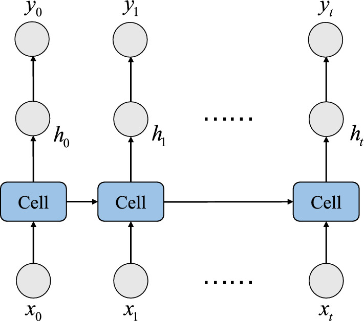
The recurrent neural network structure

The advantages of RNNs include the efficient learning ability of capturing the long-term temporal dependency and the feasibility of being combined with the attention mechanism. However, the disadvantages include the gradient vanishing and gradient explosion problems.

Convolutional neural networks

In addition to RNNs, convolutional neural networks (CNNs) can be used for time series data, e.g., 1D CNN or temporal convolutional network (TCN) shown in Fig. 5. The causal convolution operation is used in TCN, which keeps the causal relationship within time series data and only the earlier data samples would be used in a causal convolution operation as shown in Fig. 5, instead of the whole time sequence. TCNs have been proven to be a competitive alternative for RNNs in a series of prediction problems [28, 29].

Fig. 5.

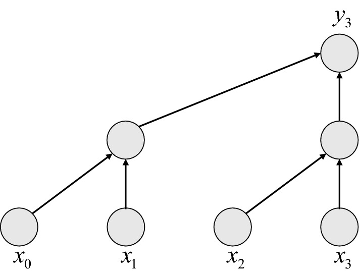
The temporal convolutional network

CNNs are also useful for capturing the spatial dependency for the input features with a grid-input format [31]. A two dimensional CNN structure is shown in Fig. 6, in which the convolution operation is conducted in a local receptive field in the convolutional layer and the neighborhood information is extracted and leveraged. Pooling or batch normalization operations can also be applied after the convolutional layer. A flattening layer is used to transform the matrices into a vector, and several dense layers are used to generate the final output. Alternatively, a global average pooling layer can be used instead of the fully connected layers.

Fig. 6.

The two-dimensional convolutional neural network structure

The advantages of CNNs include the small number of parameters and the parallel training ability with graphics processing units (GPUs). However, the disadvantages include the requirement for the Euclidean data format and the potential information loss with the pooling operation.

Graph neural networks

Since graphs are non-Euclidean data, traditional CNNs do not apply for the graph-input format. Graph neural networks (GNNs) shown in Fig. 7 are thus proposed, which have been proven effective for traffic forecasting [30]. The local convolutional operation is only conducted among the connected neighbor nodes in a graph. There are two approaches of defining the convolution kernel or the filter for GNNs, namely spectral-based and spatial-based. In the spectral-based approach, the filter is defined from graph signal processing, while in the spatial-based approach, the filter is defined with information propagation. Two representatives of GNNs include the graph convolutional network (GCN) [34] and graph attention network (GAT) [64]. GCN introduces an effective first-order approximation of Chebyshev’s spectral CNN (ChebNet) on graphs [16] and GAT further adds the attention mechanism in a graph convolutional network. GCN belongs to the spectral-based convolutional GNNs, while GAT belongs to the spatial-based convolutional GNNs.

Fig. 7.

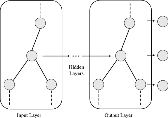
The graph neural network structure

The advantages of GNNs include the support for non-Euclidean data and the support for modeling different spatial relationships with multiple graphs. However, the disadvantages include the over-smoothing problem in training deep GNNs and the high computation requirement for huge graphs.

Time series-format models

The deep learning models used in the studies reviewed with the time series-format input are summarized in Table 2. The model components are shown in parentheses for a quick understanding of the model details. The studies reviewed are ordered by the publication year. The proposed/adopted model(s), baselines, and evaluation metrics are shown in different columns. RNNs seem to be the most suitable solution for the time series-format input case. For the baselines, both time series and machine learning models are used, including auto-regressive integrated moving average (ARIMA) and XGBoost. Historical average (HA) and moving average (MA) are two naive but competitive (at least in some cases) baselines and should be considered in relevant studies.

Table 2.

Summary of deep learning models used in the studies reviewed with the time series-format input

Study	Proposed/adopted model(s)	Baselines	Evaluation metrics
Year 2019
[50]	LSTM	DNN	RMSE
Year 2020
[91]	Memory time-series network	AR, LRidge, LSVR, GP, VAR-MLP, GRU, LSTNet	RSE, R, RMSE, MAE
[32]	TCN	ARIMA, LSTM	MAPE
[11]	LSTM, GRU	RF, FFNN	MAE, RMSE, MAPE, RMSLE
[92]	WADC (CNN+LSTM+Attention)	ARIMA, SVR, Deep Regression, CNN, SAES, LSTM, GRU, LSTM-CNN, Deep&Cross Net	RMSE, MAE, MSLE
Year 2021
[22]	Multi-Output VP-RNN	HA, MA, LR, Poisson-RNN, VP-RNN	RMSE, MAE, $R^2$
[55]	LSTM	HW, kNN	MAE, RMSE
[51]	CQRNN	N/A	RMSE, MAE, $R^2$
[72]	FFNN	N/A	MSE, $R^2$
[15]	Bi-LSTM	RF, XGBoost, DNN, LSTM	MSE, RMSE, MAPE, $R^2$

Graph-format models

The deep learning models used in the studies reviewed with the graph-format input are summarized in Table 3. GCN and GAT are both widely used for capturing spatial dependency. LSTM is more often used than GRU and TCN for capturing the temporal dependency. The attention mechanism has been proven to be an effective add-on and is widely used in the studies reviewed. Self-learned adjacency matrix for GNN-based spatiotemporal prediction is proposed recently [73], which is a promising approach and has not been fully considered for bike sharing usage prediction yet.

Table 3.

Summary of deep learning models used in the studies reviewed with the graph-format input

Study	Proposed/adopted model(s)	Baselines	Evaluation metrics
Year 2018
[7]	GraphCNN-Bike (GCN+LSTM)	HA, ARIMA, SARIMA, GBRT, LSTM	RMSE
[41]	GCNN-DDGF (GCN)	XGBoost, LSTM, MLP, SVR, LASSO, HA	RMSE, MAE, $R^2$
Year 2019
[24]	BikeNet (GCN+GRU)	ARIMA, SVR, FFNN, LSTM	RMSE, MAE, MAPE
[35]	TGNet (GN+Temporal Guided Embedding)	ARIMA, XGBoost, ST-ResNet, DMVST-Net, STDN	RMSE, MAPE, Parameter Number
[2]	STG2Seq (GCN+Attention)	HA, OLR, XGBoost, DeepST, ResST-Net, DMVST-Net, ConvLSTM, FCL-Net, FlowFLexDP, DCRNN, STGCN	RMSE, MAE, MAPE
[40]	STG2Vec+LSTM	HA, LASSO, kNN, RF, GBRT, RNN, GRU	RMSE, MAE
Year 2020
[88]	ST-CGA (GAT+CNN)	ARIMA, SVR, Fuzzy+NN, RNN, LSTM, DeepST, ST-ResNet, DMVST-Net, STDN, UrbanFM, ST-MetaNet, ST-GCN, ST-MGCN	RMSE, MAPE
[69]	SCEG (GCN)	GRU, T-GCN, E-GCN, Multi-graph, CG-GCN	MAPE, RMSPE
[18]	DTCNN (GCN+GRU)	HA, VAR, XGBoost, RNN, LSTM, GRU, DCRNN	RMSE, PCC, MAE
[58]	MVGCN (GCN)	HA, VAR, GBRT, FC-LSTM, GCN, DCRNN, FCCF, ST-MGCN	RMSE, MAE
[25]	GBikes (GAT+GCN+Attention)	HA, SHA, ARIMA, ANN, LSTM, RNN, STCNN, GC, MGN	RMSE
[46]	AGSTN (GCN+Attention+LSTM)	ARIMA, SVR, FC-LSTM, DCRNN, AST-GCN, ST-MGCN	MAE, RMSE, P@5, NDCG
[77]	BikeGAAN (GCN+Attention+LSTM)	SES, MLP, ARIMA, HA, RNN, GRU, LSTM, CNN, CNN-RNN, CNN-LSTM, CNN-GRU, GCN	MSE
[53]	GCN	HA, ARIMA, LSTM, DCRNN, STGCN	RMSE
Year 2021
[80]	GCN+GRU+Attention	XGBoost, FC-LSTM, DCRNN, STGCN, STG2Seq, Graph WaveNet	RMSE, MAE, PCC
[89]	ST-GDN (Attention+GAT+GCN)	ARIMA, SVR, Fuzzy NN, ST-RNN, D-LSTM, DeepST, ST-ResNet, DMVST-Net, STDN, UrbanFM, ST-MetaNet, DCRNN, ST-GCN, ST-MGCN, GMAN	RMSE, MAPE
[52]	GCN+LSTM	ARIMA, SVR, LSTM, DCRNN, STGCN, T-GCN	RMSE, MAE
[82]	FGST (GCN+LSTM)	FNN, LSTM, GRU, GCN	RMSE, MAE
[12]	GCN+TCN	HA, ARIMA, ETS, RF	RMSE, MAE
[47]	LSGC-LSTM (GCN+LSTM)	RNN, LSTM, GRU, GAT-LSTM, AGCRN, DGCNN	SMAPE, RMSE, MAE
[74]	STGCN (GCN+TCN)	RNN, LSTM, GRU	SMAPE, RMSE, MAE

Grid-format models

Deep learning models used in the studies reviewed with the grid-format input are summarized in Table 4. It is not surprising that CNNs are state-of-the-art solutions for capturing the spatial dependency in a grid format, which is similar to an image. It is also worth mentioning that ConvLSTM [56], a variant of LSTM with a two-dimensional input, is also widely used. In addition to ConvLSTM, other CNN-based structures are also used as the famous baselines, e.g., ST-ResNet [87] and DMVST-Net [78]. Besides the various CNN-based models, different partition sizes are also evaluated in [84].

Table 4.

Summary of deep learning models used in the studies reviewed with the grid-format input

Study	Proposed/Adopted Model(s)	Baselines	Evaluation Metrics
Year 2020
[44]	ATFM (ConvLSTM+Attention)	HA, SARIMA, VAR, ARIMA, ST-ANN, DeepST, VPN, ST-ResNet, PredNet, PredRNN	RMSE, MAE
[20]	CSCNet (CNN)	ARIMA, ConvLSTM, Peoridic-CRN, ST-ResNet, DeepSTN+	RMSE, MAE
[54]	GL-TCN (CNN+TCN)	HA, ARIMA, XGBoost, CNN, ConvLSTM, TCN, ST-ResNet, STDN	RMSE, MAE
[38]	CLTFP (CNN+LSTM)	N/A	MAPE, MAE
[76]	MBH (CNN+GRU+ConvGRU)	RNN, LSTM, GRU, ConvLSTM, ConvGRU, XGBoost, ST-ResNet, DMVST-Net	MAPE, RMSE, MAE
[71]	MT-ASTN (CNN+GCN+LSTM+Attention)	ARIMA, ConvLSTM, ST-ResNet, STDN, GEML, MDL	RMSE, MAE
[93]	ST-Attn (CNN+Attention)	ST-ANN, MNNs, ST-ResNet, ST-UNet, ConvLSTM, AttConvLSTM, PCRN	RMSE
Year 2021
[70]	CNN+GRU	HA, LR, GRU, LSTNet, ConvLSTM	RMSE, MAPE
[17]	CEST (GRU+Attention+CNN)	HA, ARIMA, GBRT, ST-ResNet, GeoMAN, CoST-Net, MiST	MAE, RMSE
[37]	STMN (ConvLSTM+CNN)	ARIMA, LSTM, ConvLSTM, STDN	RMSE, MAPE, MAE
[94]	ST-HAttn (Attention+CNN)	ARIMA, Ridge, XGBoost, ST-ANN, ST-UNet, GeoMAN, AttConvLSTM	RMSE
[86]	CNN	HA, ARIMA, SARIMA, VAR, ST-ANN, DeepST, ST-ResNet	RMSE, Training Time, Parameter Number
[67]	CNN	VAR, ARIMA, ST-ResNet, ResNet, SRCN	MAE, MSE, RMSE
[48]	ConvLSTM+LSTM	ARIMA, ConvLSTM, ST-ResNet, GEML, MDL	RMSE, MAE
[62]	ConvLSTM	N/A	MAE, RMSE, MAPE
[85]	CNN	ST-ResNet	Model Parameter, Training Time, MAE, MAPE, RMSE, $R^2$
[45]	STCL (CNN+Attention)	HA, ARIMA, VAR, MLP, FC-GRU, ConvLSTM, ST-ResNet, DMVST-Net, STDN	RMSE, MAE
[21]	STREED-Net (CNN+Attention)	HA, ST-ResNet, MST3D, 3D-CLoST, PredCNN, ST-3DNet, STAR	RMSE, MAPE, APE
[84]	DeFlow-Net (Deformable Convolution)	HA, ARIMA, ST-ResNet, ST-3DNet, T-GCN	RMSE, MASE
[23]	ASTCN (CNN+TCN+Attention)	HA, LASSO, GBDT, RF, DeepST, ST-ResNet, LSTN-PSAM, DCRNN, ST-GDN, STG2Seq	RMSE
[9]	STFNet (CNN+LSTM+Attention)	HA, ARIMA, SVR, RF, LSTM, CN	WMAPE, RMSE, MAE

Open-source projects

For replication of existing studies, open-source projects from the studies reviewed are summarized in Table 5. Two frameworks are widely used for deep learning implementation, namely TensorFlow 3 and PyTorch 4.

Table 5.

Open-source projects from the covered studies

Study	Year	Framework	Link
[7]	2018	TensorFlow	https://github.com/Di-Chai/GraphCNN-Bike
[93]	2019	TensorFlow	https://github.com/zhouyirong09/ST-Attn
[88]	2020	TensorFlow, Keras	https://github.com/jillbetty001/ST-CGA
[35]	2020	TensorFlow, Keras	https://github.com/LeeDoYup/TGGNet-keras
[69]	2020	TensorFlow	https://github.com/RoeyW/Bikes-SCEG
[44]	2020	PyTorch	https://github.com/liulingbo918/ATFM
[46]	2020	TensorFlow, Keras	https://github.com/l852888/AGSTN
[51]	2020	TensorFlow	https://github.com/inon-peled/cqrnn-pub
[92]	2020	TensorFlow, Keras	https://github.com/zhoujunhao/wadc
[80]	2021	PyTorch	https://github.com/Essaim/CGCDemandPrediction
[89]	2021	TensorFlow, Keras	https://github.com/jillbetty001/ST-GDN
[85]	2021	PyTorch	https://github.com/zhu-xm1/STPWNet
[22]	2021	PyTorch	https://github.com/DanieleGammelli/variational-poisson-rnn
[21]	2021	TensorFlow, Keras	https://github.com/UNIMIBInside/Smart-Mobility-Prediction

Auxiliary techniques

Some auxiliary techniques are further used to enhance the prediction performance of deep learning models, e.g., reinforcement learning [52], transfer learning [62], and meta learning [68]. Reinforcement learning can be used in the hyper-parameter search process, which is much better than the traditional grid search process. Transfer learning is often used in the image processing field, when the model parameters trained with a larger dataset are kept and further used in a smaller dataset. The data scarcity problem also exists in bike share systems, e.g., in cities with a new bike share system, and transfer learning techniques can be used to transfer the knowledge learned from multiple cities to this target city. Meta learning is another approach of improving the generalizability of deep learning prediction models, in which multiple meta learners can be trained first and then combined in various circumstances.

As a final word in this section, while deep learning models show a lower prediction error in most studies, a few exceptions exist. For example, a hierarchical prediction model based on a two-level fuzzy c-means clustering algorithm and a multi-similarity reference model proposed in [66] shows a better performance than RNN, LSTM, and GRU for borrow and return predictions of shared bikes.

Application scenarios

In this section, prediction-based application scenarios within and beyond bike share systems are discussed to determine the potential benefits of bike usage prediction.

Applications within bike share systems

The first application is the prediction-based recommendation system. For docked bike share systems, real-time or future bike availability information at different stations may not be provided in the original system. In this case, a prediction-based smart recommendation system can help users find an available bike with a high probability [5]. This problem is not as simple as it seems, since the user needs to make a real-time decision about which station to go, based on the future bike availability predicted, other than the current bike availability information.

The second application is choosing the facility location for new stations. In docked bike share systems, the potential demand in new stations is an important factor when choosing the ideal locations, other than the cost and accessibility considerations. Both potential demand and accessibility are used to determine where new stations should be located using a maximum covering location problem that maximizes the population served in [4] for the city of Glasgow, Scotland. Station-level interactions are further considered in [69] with GCN to capture new interactions in time-evolving station networks and the interaction pattern of new stations would be used as a reference for choosing the ideal location. The hourly bike check-ins and check-outs of functional zones, instead of bike stations, are predicted in [43]. Then the prediction results with new bike stations are used for bike sharing system expansions.

The third and last application is inventory management and bike rebalancing among different stations or regions. The imbalance of supply and demand is ubiquitous in bike share systems, especially in peak hours. The bike rebalancing problem is meaningful in both docked and dockless bike share systems and has been considered in previous studies [8, 14, 24, 42, 75]. With an effective rebalancing strategy, both the bike utilization rate and the revenue of the operator would increase. Predictive rebalancing strategies have been designed. For example, a dynamic scheduling model based on short-term check-in prediction is designed for the Chicago bike share system. A mixed integer nonlinear programming formulation of the bike routing problem is built in [42], based on the bike station pick-up and drop-off demand predictions. The relocation of damaged bikes, instead of those in a functional state, is also considered in [8] for dockless bike share systems. By removing these damaged bikes from the road, the user complaints for finding an unusable bike would decrease.

Applications beyond bike share systems

The first application is the combination with other transportation systems, especially public transit systems, e.g., bus and metro systems. For example, different management strategies for efficient land utilization are proposed in [83] for a better connection between the dockless bicycle-sharing system and the metro system in Shanghai. Another application is land usage planning and management, which is meaningful for the city planner. Bike trips can be seen as mobile and social sensors to extract land usage patterns. It has been proven useful for identifying urban space attractiveness in [3], which is a good reference for improving city land planning and management. From another perspective, different land usage plans would also affect the usage of shared bikes (and other transit systems), and the prediction results should be taken into consideration for making decisions.

Challenges and development directions

In this section, some research challenges and potential development directions are proposed to inspire the follow-up studies for usage prediction in bike share systems.

Challenges

Besides the prediction challenges discussed in Sect. 2.5, more challenges would arise when prediction models are to be used in a real-world bike share system.

The first challenge would be the use range of the prediction models proposed in the surveyed studies. Most of the existing studies evaluate the proposed method with only one or two datasets, without the guarantee the the success of an effective method in one bike share system could be replicated in another one.

The second challenge would be the prediction model deployment. Most of the surveyed studies evaluate the proposed prediction methods with historical data in an offline mode, without a full consideration for being deployed in a real-world bike share system, e.g., the deployed devices, the data collection and update methods, the user interfaces, etc.

The third challenge would be the impact of other transportation modes. As discussed in Sect. A.3, public transit usage affects the demand for shared bikes [12]. This kind of influence is bi-directional and bike sharing systems are tightly connected with other transportation modes.

Development directions

To address the above challenges, some development directions are further proposed.

Prediction with more open datasets

As shown in Table 7, only four datasets are often seen in the literature and all of them are collected from docked bike share systems. One obvious research direction is to collect and use more datasets, especially those from dockless bike share systems. However, it is both time-consuming and costly to collect new datasets. To solve this problem, more open shared bike usage datasets are summarized in Table 6, which can be used in future studies with no cost 5. The temporal ranges of these datasets are also listed for reference. It is worth mentioning that some public dockless bike sharing datasets are available, e.g., Mobike Beijing [6], ValleyBike [65] and DocklessLouisville.

Table 7.

Open datasets used in the studies reviewed

Name	Type	Link	Relevant Studies
BikeNYC	Docked	https://www.citibikenyc.com/system-data	[2, 7, 17, 18, 20–25, 35, 37, 41, 44–46, 48, 52, 54, 58, 62, 67, 69, 70, 77, 80, 82, 84–86, 88, 89, 91, 94]
BikeDC	Docked	https://www.capitalbikeshare.com/system-data	[58, 62, 69, 77, 82]
BikeChicago	Docked	https://www.divvybikes.com/system-data	[7, 17, 25, 37, 62, 77]
BikeBoston	Docked	https://academictorrents.com/details/3e395a74e333156daddcd67d614415fc9e237340	[53, 82]

Table 6.

More open datasets available for future studies

Name	Type	Link	Temporal Range
BikeLondon[61]	Docked	https://cycling.data.tfl.gov.uk/	Since April, 2015
Bike Bay Area [81]	Docked	https://github.com/TwinkleBill/babs_open_data_year_3	September 1, 2015 to August 31, 2016
BikeChattanooga	Docked	https://data.chattlibrary.org/	July 23, 2012 to April 9, 2020
Mobike Beijing [6]	Dockless	https://github.com/SharingBikeNNU/Riding-Modes_Tucker	May 10, 2017 to May 24, 2017
ValleyBike [65]	Dockless	http://traces.cs.umass.edu/index.php/Transportation/Transportation	In 2019
DocklessLouisville	Dockless	https://data.louisvilleky.gov/dataset/dockless-vehicles	Since August, 2018

Prediction for deployment

Most of the previous studies only evaluated the proposed deep learning models with numerical simulations, without deploying them in a real-world bike share system. The evaluation of the model parameter number or the training and inference time is often neglected. However, deep learning models have been criticized for both their computational complexity and the requirement of large-volume training data, both of which limit the deployment of these models in practice. Different ideas have already been proposed for better deploying a prediction model in a bike share system, for example, the idea of deploying the prediction model with cloud or edge computing. However, these early-stage ideas are far from satisfactory, and further exploration is still needed, especially those with real-world deployment experiences.

Joint prediction with other transportation modes

With the complex dynamics in a city environment, it is not sufficient to use a single type of travel demand for prediction, and some shared mobility-aware knowledge does exist in multiple travel demands [70]. For example, it is found that a majority of dockless bike trips in Singapore start from or end at metro stations [90]. Co-evolving patterns are also found between bike sharing and taxi usage in [17]. Co-prediction of taxi and bike sharing demands are further considered in [79], in which CNN is used to decompose a spatial demand into a combination of hidden spatial demand bases and LSTM is used to integrate the states of taxi and bike sharing demands. Thus, a further direction is to consider the joint prediction of bike share systems with other transportation modes. The difficulty is to collect and use heterogeneous data from different systems and data fusion techniques would be helpful in this direction.

Prediction under specific social environments

Bike sharing usage vary a lot under specific social environments, including both short-term and long-term ones. Short-term social events include both human activities and natural disasters, e.g., a flood, earthquake, or hurricane, which could last for several days or weeks. During this time period, abnormal bike sharing bike behaviors appear, making the usage less predicable or existing prediction models less reliable. Long-term social environments instead would bring a fundamental change for bike share systems, e.g., a new regulation policy. This kind of change would usually require new prediction models, instead of the existing ones which are out-of-dated.

The COVID-19 outbreak is a typical long-term social environment and has shown a wider and longer impact in our society. Lockdown and home isolation policies have been proven effective for controlling the epidemic spread, which would highly affect the demand for all kinds of transportation modes, including bike sharing. Both challenges and opportunities exist for various shared transportation modes [57]. Both positive and negative impacts on the usage of bike-sharing systems have been reported in the literature. The demand for bike share usage shows a drastic ridership reduction in New York, but the impact is less severe on the bike share system than on the subway [60]. A possible modal transfer from the subway to the bike share system is also found in the same study [60]. Another study [33] finds that bike rentals for leisure purposes rather than for means of transportation have increased during the COVID-19 pandemic. Based on a questionnaire survey conducted in the city of Thessaloniki, Greece, bike-sharing is more attractive during the COVID-19 period [49]. It would be interesting to explore whether the COVID-19 relevant situations (e.g., confirmed cases) and the lockdown policies would be useful as external factors for bike usage prediction.

Conclusion

In this survey, a comprehensive review of bike sharing usage prediction with deep learning is presented, from data collection approaches to different prediction problem types and deep learning solutions. For time series-format prediction, RNNs are state-of-the-art solutions; for graph-format prediction, GCN and GAT are two state-of-the-art solutions; and for grid-format prediction, CNNs are state-of-the-art solutions. More open datasets, various applications based on bike usage prediction and potential research directions are summarized to encourage future research.

Appendix A: Bike sharing dataset description

In this appendix, we first describe the process of collecting bike sharing data in Sect. A.1. Then some commonly used bike sharing datasets are described in Sect. A.2. The external factors used in bike sharing usage prediction problems are also summarized in Sect. A.3

A.1 Data collection

Different data collection techniques are used for docked and dockless shared bikes, as shown in Fig. 2. In most cities, a physical membership card would be necessary before using docked bikes. The trip fare can be paid once or within a monthly plan. For docked bikes, the trip records can be collected in the docking stations and then transmitted to the data center of the service operator. There are no communication devices installed in the docked bikes.

For dockless bikes, the smart lock is empowered with multiple communication functionalities. The lock is equipped with the GPS location so that the users or the maintenance team can find it easily. The lock is also equipped with the 5G connection, e.g., Massive machine-type communications (mMTC), so that the status and location of the bike is always monitored. Bluetooth can be a backup function for unlocking the bike in the case of a 5G-denied environment, e.g., in a tunnel or under a bridge. The trip record can be transmitted to the data center of the service operator in real time, and the trip fare can be paid with the smartphone application. No physical membership card is needed.

One limitation of the dockless bike is that the smart lock gradually consumes the electricity powered by a battery. The battery has a life lasting for one or two years at most. Solar cells in the basket may alleviate battery consumption but cannot change the fact that the battery must be changed to keep the dockless bike in an operational condition. This shortcoming inevitably increases the operation and maintenance cost of a dockless bike-sharing system.

A.2 Dataset description

While collected in different approaches, the trip records have a similar format for both the docked and dockless bikes. The spatial information is usually recorded as a start station id and an end station id in the docked bike system, while the station locations are generally fixed and searchable. The spatial information in a dockless bike system is usually the start and end GPS coordinates for a single trip. Geo-coding techniques may be applied to transform the precise location to a broader region to protect user privacy. The temporal information is usually the start and end timestamps for a single trip. Other attributes can be collected, but may not be relevant to usage prediction purposes, e.g., bike id, user id, trip fare, etc.

To regulate and support the bike-sharing systems, the relevant government departments are also defining and unifying the trip data format. For example, the General Bikeshare Feed Specification (GBFS) 6 is defined as the open data standard for shared bikes and makes real-time data feeds in a uniform format publicly available online, with an emphasis on findability. The GBFS has been adopted in more than 12 cities in North America.

Many bike-sharing systems release their accumulated trip records regularly, e.g., monthly or yearly. Some famous open datasets are widely used in the studies reviewed. A list of the open datasets used in the reviewed studies is shown in Table 7. The datasets in Table 7 are all collected in docked bike share systems, from four different cities, namely New York, Washington, Chicago, and Boston. All four datasets have been collected for a long time, e.g., BikeNYC, BikeDC and BikeBoston can be dated back to 2011, and BikeChicago can be dated back to 2015. The station numbers also changed as new stations were added and some old stations were removed. For example, the NYC Bike System contains 416 stations and the Washington D.C. Bike System contains 472 stations at the time when this survey is in preparation.

The relevant studies using these open datasets are also listed in Table 7. Since these bike-sharing systems are still in operation and trip records continue to grow, different studies may use these datasets with a different time range, making the prediction results less comparable.

A.3 External factors

Bike usage prediction is mainly based on the temporal and spatial dependencies learned from historical data. Many external factors would also affect the bike-sharing demand and should be considered in building an effective prediction model [19]. The effect of each external factor for prediction is considered in [10] and the combination of different external factors is also considered in [55].

External factors used in the studies reviewed are summarized in Table 8. Bike usage is more affected by the weather factor than other transportation modes, e.g., and it is not suitable for riding a bike on a rainy or windy day. The calendar factor includes the time of day, weekdays, weekends, and holidays. For those who ride the shared bike on weekdays, there are obvious to-work and to-home patterns in morning and evening peak hours. These patterns would be totally different on weekends or holidays. The point of interest (POI) or land usage situation around the station or within a region is also used, which reflects the potential need for bike usage, e.g., riding from a metro station to the places of interest.

Table 8.

External factors used in the studies reviewed

Type	Relevant studies
Weather	[7, 9, 11, 18, 21, 23, 25, 44, 48, 54, 55, 58, 69, 70, 76, 77, 88, 89]
Calendar	[11, 18, 21, 25, 44, 48, 54, 55, 58, 69–71, 76, 88, 89]
PoI	[9, 25, 48, 71, 76, 77]
Air Quality	[9]
Social Event	[77]
Land Usage	[12]
Public Transit Usage	[12]
Traffic Accident	[45]

Other external factors are also used, although in rare cases. Similar to the weather factor, air quality is another factor that affects bike-riding willingness, especially in cities with severe pollution. Social events affect the overall transportation system, including the bike share system. For example, the traffic demand would increase dramatically around a stadium after a match, with the audience going home. Use with other public transit systems would also affect the need for shared bikes with the similar purpose of short-distance trips, e.g., buses and subways. Finally, traffic accidents adversely affect the usage of road vehicles, e.g., buses and taxis, and bikes can be used as a potential alternative in cases of road congestion or emergencies.

The difficulty of obtaining these external factors is totally different. It is easy to find the weather, calendar, air quality or public transit usage data sources that are published by the government or commercial companies, with or without a cost. The PoI data can be obtained from map service providers and there are some non-commercial options, e.g., OpenStreetMap. Land usage data can be extracted from government documents, which usually require more manual processing work than well-formatted PoI data. It is not easy to obtain social event and traffic accident data in real time. Previous studies have used natural language processing and keyword matching techniques to extract relevant event or accident information from social media data, e.g., Twitter or Facebook.

The update frequency of these external factors also varies. The weather, calendar, air quality and public transmit usage data can be updated daily or hourly. The social event and traffic accident data have no regular update frequency. The POI and land usage data would stay the same for a long time period, e.g., months or even years.

Declarations

Conflict of interest

The authors declare that they have no conflict of interest.

References

- 1.Albuquerque V, Sales Dias M, Bacao F. Machine learning approaches to bike-sharing systems: a systematic literature review. ISPRS Int J Geo Inf. 2021;10(2):62. doi: 10.3390/ijgi10020062. [DOI] [Google Scholar]
- 2.Bai L, Yao L, Kanhere SS, et al (2019) Stg2seq: spatial-temporal graph to sequence model for multi-step passenger demand forecasting. In: Proceedings of the 28th international joint conference on artificial intelligence, AAAI Press, pp 1981–1987
- 3.Banet K, Naumov V, Kucharski R (2021) Using city-bike stopovers to reveal spatial patterns of urban attractiveness. Current Issues in Tourism pp 1–18
- 4.Beairsto J, Tian Y, Zheng L, et al (2021) Identifying locations for new bike-sharing stations in Glasgow: an analysis of spatial equity and demand factors. Annals of GIS pp 1–16
- 5.Billhardt H, Fernández A, Ossowski S. Smart recommendations for renting bikes in bike-sharing systems. Appl Sci. 2021;11(20):9654. doi: 10.3390/app11209654. [DOI] [Google Scholar]
- 6.Cao M, Huang M, Ma S, et al. Analysis of the spatiotemporal riding modes of dockless shared bicycles based on tensor decomposition. Int J Geogr Inf Sci. 2020;34(11):2225–2242. doi: 10.1080/13658816.2020.1768259. [DOI] [Google Scholar]
- 7.Chai D, Wang L, Yang Q (2018) Bike flow prediction with multi-graph convolutional networks. In: Proceedings of the 26th ACM SIGSPATIAL international conference on advances in geographic information systems, pp 397–400
- 8.Chang X, Wu J, Sun H, et al. Relocating operational and damaged bikes in free-floating systems: a data-driven modeling framework for level of service enhancement. Transp Res Part A Policy Pract. 2021;153:235–260. doi: 10.1016/j.tra.2021.09.010. [DOI] [Google Scholar]
- 9.Chang X, Wu J, Sun H, et al (2021) Understanding and predicting short-term passenger flow of station-free shared bike: a spatiotemporal deep learning approach. IEEE Intelligent Transportation Systems Magazine
- 10.Chen L, Wang L (2021) Exploring context modeling techniques on the spatiotemporal crowd flow prediction. arXiv preprint arXiv:210616046
- 11.Chen PC, Hsieh HY, Su KW, et al. Predicting station level demand in a bike-sharing system using recurrent neural networks. IET Intell Transp Syst. 2020;14(6):554–561. doi: 10.1049/iet-its.2019.0007. [DOI] [Google Scholar]
- 12.Cho JH, Ham SW, Kim DK (2021) Enhancing the accuracy of peak hourly demand in bike-sharing systems using a graph convolutional network with public transit usage data. Transp Res Record p 03611981211012003
- 13.Cho K, Van Merriënboer B, Gulcehre C, et al (2014) Learning phrase representations using rnn encoder-decoder for statistical machine translation. arXiv preprint arXiv:14061078
- 14.Cipriano M, Colomba L, Garza P. A data-driven based dynamic rebalancing methodology for bike sharing systems. Appl Sci. 2021;11(15):6967. doi: 10.3390/app11156967. [DOI] [Google Scholar]
- 15.Collini E, Nesi P, Pantaleo G. Deep learning for short-term prediction of available bikes on bike-sharing stations. IEEE Access. 2021;9:124-337–124-347. doi: 10.1109/ACCESS.2021.3110794. [DOI] [Google Scholar]
- 16.Defferrard M, Bresson X, Vandergheynst P (2016) Convolutional neural networks on graphs with fast localized spectral filtering. In: Proceedings of the 30th international conference on neural information processing systems, pp 3844–3852
- 17.Deng J, Chen X, Fan Z, et al. The pulse of urban transport: exploring the co-evolving pattern for spatio-temporal forecasting. ACM Trans Knowl Discov Data. 2021;15(6):1–25. doi: 10.1145/3450528. [DOI] [Google Scholar]
- 18.Du B, Hu X, Sun L, et al. Traffic demand prediction based on dynamic transition convolutional neural network. IEEE Trans Intell Transp Syst. 2020;22(2):1237–1247. doi: 10.1109/TITS.2020.2966498. [DOI] [Google Scholar]
- 19.Eren E, Uz VE. A review on bike-sharing: the factors affecting bike-sharing demand. Sustain Cities Soc. 2020;54(101):882. [Google Scholar]
- 20.Feng J, Lin Z, Xia T, et al (2020) A sequential convolution network for population flow prediction with explicitly correlation modelling. In: IJCAI, pp 1331–1337
- 21.Fiorini S, Ciavotta M, Maurino A (2021) Listening to the city, attentively: A spatio-temporal attention boosted autoencoder for the short-term flow prediction problem. arXiv preprint arXiv:210300983
- 22.Gammelli D, Wang Y, Prak D, et al. Predictive and prescriptive performance of bike-sharing demand forecasts for inventory management. Transp Res Part C: Emerg Technol. 2022;138(103):571. [Google Scholar]
- 23.Guo H, Zhang D, Jiang L, et al. Astcn: an attentive spatial temporal convolutional network for flow prediction. IEEE Internet Things J. 2021;9:3215–3225. doi: 10.1109/JIOT.2021.3100068. [DOI] [Google Scholar]
- 24.Guo R, Jiang Z, Huang J et al (2019) Bikenet: accurate bike demand prediction using graph neural networks for station rebalancing. In: 2019 IEEE smartworld, ubiquitous intelligence & computing, advanced & trusted computing, scalable computing & communications. cloud & big data computing, internet of people and smart city innovation (SmartWorld/SCALCOM/UIC/ATC/CBDCom/IOP/SCI), IEEE, pp 686–693
- 25.He S, Shin KG (2020) Towards fine-grained flow forecasting: a graph attention approach for bike sharing systems. In: Proceedings of the web conference 2020. association for computing machinery, New York, NY, USA, WWW ’20, p 88–98. 10.1145/3366423.3380097 [DOI]
- 26.Hochreiter S, Schmidhuber J. Long short-term memory. Neural Comput. 1997;9(8):1735–1780. doi: 10.1162/neco.1997.9.8.1735. [DOI] [PubMed] [Google Scholar]
- 27.Jiang M, Li C, Li K, et al. Destination prediction based on virtual poi docks in dockless bike-sharing system. IEEE Trans Intell Transp Syst. 2021;23:2457–2470. doi: 10.1109/TITS.2021.3099571. [DOI] [Google Scholar]
- 28.Jiang W. Applications of deep learning in stock market prediction: recent progress. Expert Syst Appl. 2021;184:115537. doi: 10.1016/j.eswa.2021.115537. [DOI] [Google Scholar]
- 29.Jiang W. Internet traffic prediction with deep neural networks. Internet Technol Lett. 2021;5:e314. [Google Scholar]
- 30.Jiang W, Luo J (2021) Graph neural network for traffic forecasting: a survey. arXiv preprint arXiv:210111174
- 31.Jiang W, Zhang L. Geospatial data to images: a deep-learning framework for traffic forecasting. Tsinghua Sci Technol. 2018;24(1):52–64. doi: 10.26599/TST.2018.9010033. [DOI] [Google Scholar]
- 32.Jin K, Wang W, Li S, et al. Dockless shared-bike demand prediction with temporal convolutional networks. CICTP. 2020;2020:2851–2863. [Google Scholar]
- 33.Kim K. Impact of covid-19 on usage patterns of a bike-sharing system: case study of seoul. J Transp Eng, Part A: Syst. 2021;147(10):05021006. doi: 10.1061/JTEPBS.0000591. [DOI] [Google Scholar]
- 34.Kipf TN, Welling M (2017) Semi-supervised classification with graph convolutional networks. In: International conference on learning representations (ICLR ’17)
- 35.Lee D, Jung S, Cheon Y, et al (2019) Demand forecasting from spatiotemporal data with graph networks and temporal-guided embedding. arXiv preprint arXiv:190510709
- 36.Lee K, Eo M, Jung E, et al (2021) Short-term traffic prediction with deep neural networks: a survey. IEEE Access 9:54,739–54,756
- 37.Li X, Xu Y, Chen Q, et al (2021) Short-term forecast of bicycle usage in bike sharing systems: a spatial-temporal memory network. IEEE Trans Intell Transp Syst
- 38.Li Y, Shuai B. Origin and destination forecasting on dockless shared bicycle in a hybrid deep-learning algorithms. Multimed Tools Appl. 2020;79(7):5269–5280. doi: 10.1007/s11042-018-6374-x. [DOI] [Google Scholar]
- 39.Li Y, Zheng Y, Zhang H, et al (2015) Traffic prediction in a bike-sharing system. In: Proceedings of the 23rd SIGSPATIAL international conference on advances in geographic information systems, pp 1–10
- 40.Li Y, Zhu Z, Kong D, et al (2019) Learning heterogeneous spatial-temporal representation for bike-sharing demand prediction. In: Proceedings of the AAAI conference on artificial intelligence, pp 1004–1011
- 41.Lin L, He Z, Peeta S. Predicting station-level hourly demand in a large-scale bike-sharing network: a graph convolutional neural network approach. Transp Res Part C Emerging Technol. 2018;97:258–276. doi: 10.1016/j.trc.2018.10.011. [DOI] [Google Scholar]
- 42.Liu J, Sun L, Chen W, et al (2016) Rebalancing bike sharing systems: a multi-source data smart optimization. In: Proceedings of the 22nd ACM SIGKDD international conference on knowledge discovery and data mining, pp 1005–1014
- 43.Liu J, Sun L, Li Q, et al (2017) Functional zone based hierarchical demand prediction for bike system expansion. In: Proceedings of the 23rd ACM SIGKDD international conference on knowledge discovery and data mining, pp 957–966
- 44.Liu L, Zhen J, Li G, et al (2020) Dynamic spatial-temporal representation learning for traffic flow prediction. IEEE Trans Intell Transp Syst
- 45.Liu Z, Zhang R, Wang C, et al (2021) Spatial-temporal conv-sequence learning with accident encoding for traffic flow prediction. arXiv preprint arXiv:210510478
- 46.Lu YJ, Li CT (2020) Agstn: Learning attention-adjusted graph spatio-temporal networks for short-term urban sensor value forecasting. In: 2020 IEEE international conference on data mining (ICDM), IEEE, pp 1148–1153
- 47.Luo J, Zhou D, Han Z, et al. Predicting travel demand of a docked bikesharing system based on LSGC-LSTM networks. IEEE Access. 2021;9:92,189–92,203. doi: 10.1109/ACCESS.2021.3062778. [DOI] [Google Scholar]
- 48.Miao H, Fei Y, Wang S, et al (2021) Deep learning based origin-destination prediction via contextual information fusion. Multimed Tools Appl pp 1–17
- 49.Nikiforiadis A, Ayfantopoulou G, Stamelou A. Assessing the impact of COVID-19 on bike-sharing usage: the case of Thessaloniki, Greece. Sustainability. 2020;12(19):8215. doi: 10.3390/su12198215. [DOI] [Google Scholar]
- 50.Pan Y, Zheng RC, Zhang J, et al. Predicting bike sharing demand using recurrent neural networks. Procedia Comput Sci. 2019;147:562–566. doi: 10.1016/j.procs.2019.01.217. [DOI] [Google Scholar]
- 51.Peled I, Rodrigues F, Pereira FC (2021) Modeling censored mobility demand through quantile regression neural networks. arXiv preprint arXiv:210401214
- 52.Peng H, Du B, Liu M, et al. Dynamic graph convolutional network for long-term traffic flow prediction with reinforcement learning. Inf Sci. 2021;578:401–416. doi: 10.1016/j.ins.2021.07.007. [DOI] [Google Scholar]
- 53.Qin T, Liu T, Wu H, et al (2020) Resgcn: residual graph convolutional network based free dock prediction in bike sharing system. In: 2020 21st IEEE international conference on mobile data management (MDM), IEEE, pp 210–217
- 54.Ren Y, Zhao D, Luo D, et al (2020) Global-local temporal convolutional network for traffic flow prediction. IEEE Trans Intell Transp Syst
- 55.Sardinha C, Finamore AC, Henriques R (2021) Context-aware demand prediction in bike sharing systems: incorporating spatial, meteorological and calendrical context. arXiv preprint arXiv:210501125
- 56.Shi X, Chen Z, Wang H, et al (2015) Convolutional lstm network: A machine learning approach for precipitation nowcasting. Adv Neural Inf Process Syst 28
- 57.Shokouhyar S, Shokoohyar S, Sobhani A, et al. Shared mobility in post-COVID era: New challenges and opportunities. Sustain Cities Soc. 2021;67(102):714. doi: 10.1016/j.scs.2021.102714. [DOI] [PMC free article] [PubMed] [Google Scholar]
- 58.Sun J, Zhang J, Li Q, et al (2020) Predicting citywide crowd flows in irregular regions using multi-view graph convolutional networks. IEEE Tran Knowl Data Eng
- 59.Tedjopurnomo DA, Bao Z, Zheng B, et al. A survey on modern deep neural network for traffic prediction: trends, methods and challenges. IEEE Trans Knowl Data Eng. 2020;34:1544–1561. [Google Scholar]
- 60.Teixeira JF, Lopes M. The link between bike sharing and subway use during the COVID-19 pandemic: the case-study of New York’s Citi Bike. Transp Res Interdiscip Perspect. 2020;6(100):166. doi: 10.1016/j.trip.2020.100166. [DOI] [PMC free article] [PubMed] [Google Scholar]
- 61.Tekouabou SCK, et al. Intelligent management of bike sharing in smart cities using machine learning and internet of things. Sustain Cities Soc. 2021;67(102):702. [Google Scholar]
- 62.Tian C, Zhu X, Hu Z, et al. A transfer approach with attention reptile method and long-term generation mechanism for few-shot traffic prediction. Neurocomputing. 2021;452:15–27. doi: 10.1016/j.neucom.2021.03.068. [DOI] [Google Scholar]
- 63.Vaswani A, Shazeer N, Parmar N, et al (2017) Attention is all you need. arXiv preprint arXiv:170603762
- 64.Veličković P, Cucurull G, Casanova A, et al (2018) Graph attention networks. In: International conference on learning representations
- 65.Wamburu J, Raff C, Irwin D, et al (2020) Greening electric bike sharing using solar charging stations. In: Proceedings of the 7th ACM international conference on systems for energy-efficient buildings, cities, and transportation, pp 180–189
- 66.Wang B, Tan Y, Jia W. Tl-fcm: a hierarchical prediction model based on two-level fuzzy c-means clustering for bike-sharing system. Appl Intell. 2021;52:1–18. [Google Scholar]
- 67.Wang B, Vu HL, Kim I, et al (2021) Short-term traffic flow prediction in bike-sharing networks. J Intell Transp Syst pp 1–18
- 68.Wang L, Chai D, Liu X, et al (2021) Exploring the generalizability of spatio-temporal traffic prediction: meta-modeling and an analytic framework. IEEE Trans Knowl Data Eng
- 69.Wang Q, Guo B, Ouyang Y, et al (2020) Spatial community-informed evolving graphs for demand prediction. In: Proceedings of The European conference on machine learning and principles and practice of knowledge discovery in databases (ECML-PKDD 2020), pp 440–456
- 70.Wang Q, Guo B, Ouyang Y, et al. Learning shared mobility-aware knowledge for multiple urban travel demands. IEEE Internet Things J. 2021;9:7025–7035. doi: 10.1109/JIOT.2021.3115174. [DOI] [Google Scholar]
- 71.Wang S, Miao H, Chen H, et al (2020) Multi-task adversarial spatial-temporal networks for crowd flow prediction. In: Proceedings of the 29th ACM international conference on information & knowledge management, pp 1555–1564
- 72.Wu F, Hong S, Zhao W, et al. Neural networks with improved extreme learning machine for demand prediction of bike-sharing. Mobile Netw Appl. 2021;26:1–11. doi: 10.1007/s11036-021-01737-1. [DOI] [Google Scholar]
- 73.Wu Z, Pan S, Long G, et al (2020) Connecting the dots: Multivariate time series forecasting with graph neural networks. In: Proceedings of the 26th ACM SIGKDD international conference on knowledge discovery & data mining, pp 753–763
- 74.Xiao G, Wang R, Zhang C, et al. Demand prediction for a public bike sharing program based on spatio-temporal graph convolutional networks. Multimed Tools Appl. 2021;80(15):22907–22925. doi: 10.1007/s11042-020-08803-y. [DOI] [Google Scholar]
- 75.Xu H, Duan F, Pu P. Dynamic bicycle scheduling problem based on short-term demand prediction. Appl Intell. 2019;49(5):1968–1981. doi: 10.1007/s10489-018-1360-6. [DOI] [Google Scholar]
- 76.Xu M, Liu H, Yang H. A deep learning based multi-block hybrid model for bike-sharing supply-demand prediction. IEEE Access. 2020;8:85826–85838. doi: 10.1109/ACCESS.2020.2987934. [DOI] [Google Scholar]
- 77.Yang X, He S, Huang H (2020) Station correlation attention learning for data-driven bike sharing system usage prediction. In: 2020 IEEE 17th international conference on mobile ad hoc and sensor systems (MASS), IEEE, pp 640–648
- 78.Yao H, Wu F, Ke J, et al (2018) Deep multi-view spatial-temporal network for taxi demand prediction. In: Proceedings of the AAAI conference on artificial intelligence
- 79.Ye J, Sun L, Du B, et al (2019) Co-prediction of multiple transportation demands based on deep spatio-temporal neural network. In: Proceedings of the 25th ACM SIGKDD international conference on knowledge discovery & data mining, pp 305–313
- 80.Ye J, Sun L, Du B, et al (2021) Coupled layer-wise graph convolution for transportation demand prediction. In: Proceedings of the AAAI conference on artificial intelligence, pp 4617–4625
- 81.Yi P, Huang F, Peng J. A rebalancing strategy for the imbalance problem in bike-sharing systems. Energies. 2019;12(13):2578. doi: 10.3390/en12132578. [DOI] [Google Scholar]
- 82.Yi P, Huang F, Peng J (2021) A fine-grained graph-based spatiotemporal network for bike flow prediction in bike-sharing systems. In: Proceedings of the 2021 SIAM international conference on data mining (SDM), SIAM, pp 513–521
- 83.Yu Q, Li W, Yang D, et al. Policy zoning for efficient land utilization based on spatio-temporal integration between the bicycle-sharing service and the metro transit. Sustainability. 2021;13(1):141. doi: 10.3390/su13010141. [DOI] [Google Scholar]
- 84.Zeng W, Lin C, Liu K, et al (2021) Modeling spatial nonstationarity via deformable convolutions for deep traffic flow prediction. IEEE Trans Knowl Data Eng
- 85.Zhai L, Yang Y, Song S, et al. Self-supervision spatiotemporal part-whole convolutional neural network for traffic prediction. Physica A: Stat Mech Appl. 2021;579:126141. doi: 10.1016/j.physa.2021.126141. [DOI] [Google Scholar]
- 86.Zhai Z, Liu P, Zhao L, et al. An efficiency-enhanced deep learning model for citywide crowd flows prediction. Int J Mach Learn Cybern. 2021;12:1–13. doi: 10.1007/s13042-021-01282-z. [DOI] [Google Scholar]
- 87.Zhang J, Zheng Y, Qi D (2017) Deep spatio-temporal residual networks for citywide crowd flows prediction. In: Proceedings of the AAAI conference on artificial intelligence
- 88.Zhang X, Huang C, Xu Y, et al (2020) Spatial-temporal convolutional graph attention networks for citywide traffic flow forecasting. In: Proceedings of the 29th ACM international conference on information & knowledge management, pp 1853–1862
- 89.Zhang X, Huang C, Xu Y, et al (2021) Traffic flow forecasting with spatial-temporal graph diffusion network. In: Proceedings of the AAAI conference on artificial intelligence, pp 15,008–15,015
- 90.Zhang X, Shen Y, Zhao J. The mobility pattern of dockless bike sharing: A four-month study in Singapore. Transp Res Part D: Transp Environ. 2021;98(102):961. [Google Scholar]
- 91.Zhao S, Lin S, Li Y, et al (2020) Urban traffic flow forecasting based on memory time-series network. In: 2020 IEEE 23rd international conference on intelligent transportation systems (ITSC), IEEE, pp 1–6
- 92.Zhou J, Dai HN, Wang H, et al. Wide-attention and deep-composite model for traffic flow prediction in transportation cyber-physical systems. IEEE Trans Industr Inf. 2020;17(5):3431–3440. doi: 10.1109/TII.2020.3003133. [DOI] [Google Scholar]
- 93.Zhou Y, Li J, Chen H, et al. A spatiotemporal attention mechanism-based model for multi-step citywide passenger demand prediction. Inf Sci. 2020;513:372–385. doi: 10.1016/j.ins.2019.10.071. [DOI] [Google Scholar]
- 94.Zhou Y, Li J, Chen H, et al. A spatiotemporal hierarchical attention mechanism-based model for multi-step station-level crowd flow prediction. Inf Sci. 2021;544:308–324. doi: 10.1016/j.ins.2020.07.049. [DOI] [Google Scholar]