MR Parameter Mapping Using Model-Guided Self-Supervised Deep Learning

Abstract

Purpose:

To develop a model-guided self-supervised deep learning MRI reconstruction framework called REference-free LAtent map eXtraction (RELAX) for rapid quantitative MR parameter mapping.

Methods:

Two physical models are incorporated for network training in RELAX, including the inherent MR imaging model and a quantitative model that is used to fit parameters in quantitative MRI. By enforcing these physical model constraints, RELAX eliminates the need for full sampled reference datasets that are required in standard supervised learning. Meanwhile, RELAX also enables direct reconstruction of corresponding MR parameter maps from undersampled k-space. Generic sparsity constraints used in conventional iterative reconstruction, such as the total variation constraint, can be additionally included in the RELAX framework to improve reconstruction quality. The performance of RELAX was tested for accelerated T1 and T2 mapping in both simulated and actually-acquired MRI datasets and was compared with supervised learning and conventional constrained reconstruction for suppressing noise and/or undersampling-induced artifacts.

Results:

In the simulated datasets, RELAX generated good T1/T2 maps in the presence of noise and/or undersampling artifacts comparable to artifact/noise-free ground truth. The inclusion of a spatial total variation constraint helps improve image quality. For the in-vivo T1/T2 mapping datasets, RELAX achieved superior reconstruction quality compared to conventional iterative reconstruction and similar reconstruction performance to supervised deep learning reconstruction.

Conclusion:

This work has demonstrated the initial feasibility of rapid quantitative MR parameter mapping based on self-supervised deep learning. The RELAX framework may also be further extended to other quantitative MRI applications by incorporating corresponding quantitative imaging models.

INTRODUCTION

The use of deep learning for reconstructing undersampled MR images has gained substantial interest and attention in recent years (1–5). Deep learning utilizes a unique architecture (e.g., convolutional neural network (CNN)) (6) for extracting image features from reference MRI datasets with a data-driven training strategy, which enables more effective removal of undersampling artifacts/noise compared to standard constrained MRI reconstruction (e.g., compressed sensing reconstruction) that typically relies on generic image priors. Meanwhile, once the training step is completed, the learned deep neural networks are fixed and allow for rapid inference (reconstruction) of new undersampled datasets, typically in the order of seconds. This offers a unique opportunity to facilitate fast MRI reconstruction into routine clinical use from an efficient computation perspective.

To date, most deep learning-based MRI reconstruction techniques are based on a supervised training strategy, which aims to learn the mapping of undersampled images (with artifacts and noises) to corresponding reference images (typically fully sampled) with CNNs(1–5). One major challenge of supervised learning, however, is the requirement of abundant high-quality reference images for network training. Although fully sampled static MR images may be obtained from routine MRI exams, it can be significantly challenging to acquire fully sampled dynamic MRI due to motion, imaging speed restriction, and associated trade-off between spatiotemporal resolution and volumetric coverage that must be made in many dynamic imaging applications. In addition, ground truth images for quantitative MRI (e.g., MR relaxometry) are also difficult to acquire because quantitative imaging typically requires prolonged imaging time and it is not routinely implemented in current clinical settings. As a result, the requirement of reference images for network training can greatly restrict the broad applications of supervised learning in MRI reconstruction, particularly for dynamic or quantitative MRI.

More recently, several works have investigated unsupervised or self-supervised learning for the reconstruction of undersampled static MR images (7–12). Although the specific implementations of these works vary from one to the other, they all train CNNs on undersampled datasets directly without fully-sampled references, and inherent MR physical models (e.g., Fourier encoding and coil sensitivity encoding) are incorporated as training regularizations. The results in these works have shown that with proper design of network training, unsupervised or self-supervised learning can achieve similar reconstruction performance compared to supervised learning (8,9,11,12). In addition to standard Fourier and coil encoding for static image reconstruction, MRI also offers a variety of physical models that are typically used in quantitative MRI and can be exploited for deep learning reconstruction of quantitative images. Examples of these models include MR relaxometry models for T1 or T2 mapping, diffusion models for diffusion parameter mapping, and tissue susceptibility models for quantitative susceptibility imaging. While the use of these models in conventional iterative reconstruction (the so-called model-based reconstruction (13–17)) has been well demonstrated in the literature, their use in deep learning-based MRI reconstruction has been very limited (18), particularly in the context of self-supervised learning.

The purpose of this study was to propose a general self-supervised deep learning reconstruction framework for quantitative MRI. This technique, called REference-free LAtent map eXtraction (RELAX), jointly enforces data-driven and physics-driven training, where the MR imaging model (Fourier encoding/coil sensitivity encoding) and a quantitative model are incorporated in network training towards self-supervised deep learning reconstruction. The demonstration of RELAX was tailored explicitly for rapid MR T1 and T2 mapping in this work. In the following sections, the framework of RELAX is first presented. Its performance is then demonstrated in realistic simulation studies followed by in-vivo evaluation of accelerated T1 and T2 mapping of the knee joint.

THEORY

Deep Learning Reconstruction with Supervised Learning

Deep learning enables direct end-to-end mapping for domain-to-domain translations using CNNs. The mechanism of end-to-end mapping is to train a CNN for learning spatial or spatiotemporal features, correlations, and contrast relationships between input datasets and desirable outputs. Once the training is completed, the learned networks can then be employed to efficiently inference new input data. When deep learning is applied to reconstruct accelerated MRI data, the inputs can be pairs of undersampled images with aliasing artifacts and corresponding fully sampled images (e.g., k-space sampling satisfying the Nyquist requirement). A learned network can then be applied to reconstruct new undersampled images by removing aliasing artifacts. Mathematically, this framework can be formulated as the following optimization function:

$$\tilde{\theta }=\text{arg\hspace{0.17em}}\underset{\theta }{\text{min}}\left({\mathbb{E}}_{d_u~P(d_u)}\left[{\Vert C({\mathbf{\text{d}}}_u|\theta )-\mathbf{\text{d}}\Vert }_K\right]\right)$$ [1]

Here, $C\left(d_u|\theta \right):d_u\to \tilde{d}$ is an end-to-end CNN generator conditioned on network parameters θ, so that it generates image $\tilde{d}$ from undersampled image d_u. d represents reference fully sampled images for network training. ${\mathbb{E}}_{d_u~P(d_u)}[\cdot ]$ is an expectation operator given that a training sample d_u belongs to the data distribution P(d_u) of all undersampled image datasets. ‖·‖_K forms a loss function, where K is typically set as 1 or 2 representing ℓ₁ or ℓ₂ norm. The network aims to search for optimized parameters θ through data-driven training, which can be generalized and applied to other new undersampled images. Since there is an explicit requirement for reference images in Eq.[1], this framework is generally referred to as supervised learning.

Model-Based Deep Learning Reconstruction with Supervised Learning

The performance of deep learning-based MRI reconstruction can be further improved by incorporating additional constraints considering physical models that are inherently available in MRI. These constraints ensure that images generated from CNN mapping must be consistent with both the training reference and also corresponding physical models. A typical model that can be considered is MR imaging encoding (e.g., Fourier encoding), an essential process that is embedded in all MRI data acquisition and reconstruction. With this extension, Eq.[1] then becomes:

$$\tilde{\theta }=\text{arg\hspace{0.17em}}\underset{\theta }{\text{min}}\left({\lambda }_{\mathit{\text{loss}}1}{\mathbb{E}}_{d_u~P(d_u)}\left[{\Vert \mathbf{\text{E}}C({\mathbf{\text{d}}}_u|\theta )-y_u\Vert }_K\right]+{\lambda }_{\mathit{\text{loss}}2}{\mathbb{E}}_{d_u~P(d_u)}\left[{\Vert C({\mathbf{\text{d}}}_u|\theta )-\mathbf{\text{d}}\Vert }_K\right]\right)$$ [2]

Here, y_u denotes undersampled k-space and E is a forward model describing imaging encoding, which can include the Fourier transform, coil sensitivities (when multi-coil arrays are used), and undersampling patterns to generate y_u. Compared to Eq.[1] with only a single loss term, Eq.[2] promotes data fidelity by further ensuring that CNN-generated images need to be consistent with acquired undersampled k-space. It can be seen that Eq.[2] is in close analogy to conventional constrained reconstruction. In fact, the right loss term in Eq.[2] can be treated as a regularization function to perform constrained image reconstruction. This leads to a joint data-driven and model-driven deep learning reconstruction framework balanced by two weighting parameters λ_loss1 and λ_loss2. Although some deep learning reconstruction methods are based on Eq.[1] (19–21), most recent deep learning techniques are based on Eq.[2] to fully take advantage of the MRI encoding process (1,3,5,22–24).

Model-Based Deep Learning Reconstruction with Self-Supervised Learning

The incorporation of MR physical models into deep learning MRI reconstruction in Eq.[2] not only improves the performance of supervised learning but also offers an opportunity to perform network training without the need for fully sampled references. In this scenario, CNN learning can be formulated by adapting Eq.[2] to eliminate the right loss term that relies on references, leaving the left data consistency term to enforce “self-supervision”:

$$\tilde{\theta }=\text{arg\hspace{0.17em}}\underset{\theta }{\text{min}}\left({\mathbb{E}}_{d_u~P(d_u)}\left[{\Vert \mathbf{\text{E}}C({\mathbf{\text{d}}}_u|\theta )-y_u\Vert }_K\right]\right)$$ [3]

The training of Eq.[3] purely relies on the imaging encoding mechanisms of MRI to find out how to remove undersampling-induced artifacts and noises. In this manner, self-supervised learning still enforces a joint data-driven (a training database consisting of only undersampled images) and model-driven network training process, but it is implemented in a relaxed and weaker manner without fully sampled reference. This generic framework forms an undersampling-to-undersampling training strategy that closely resembles an early work using noise-to-noise training for imaging denoising in computer vision (7). It has been proven feasible in reconstructing undersampled MR images and was found to achieve reconstruction performance that is similar to standard supervised learning (9,12). It can also be adapted for special training designs for further improved reconstruction performance. For example, a more recent work (11) further employs a training strategy by splitting undersampled k-space into two parts, such that y_u = y_ui + y_uj. During network training, y_ui can be used as the CNN input while y_uj can be employed for calculating the training loss.

RELAX: Quantitative Deep Learning Reconstruction with Model-Based Self-Supervised Learning

In addition to standard imaging encoding, other models can also be further incorporated into deep learning reconstruction. For example, quantitative MRI typically replies on an MR signal model to generate quantitative parameters based on the following equation:

$$\tilde{\Delta }=\text{arg\hspace{0.17em}}\underset{\Delta }{\text{min}}{\Vert \mathbf{\text{M}}(\Delta )-\mathbf{\text{d}}\Vert }_2$$ [4]

where M represents a quantitative signal model (e.g., a T1 relaxation or T2 decaying model for MR relaxometry) to fit a series of multi-contrast images d into corresponding quantitative parameters, denoted as Δ here. Please note that throughout this paper, “multi-contrast” is specifically referred to as multiple k-space/images acquired with different imaging parameters (e.g., different echo times or different flip angles) to fit quantitative MR parameters. This quantitative signal model can be embedded into deep learning reconstruction to enforce a model constraint. Meanwhile, the use of a quantitative signal model also enables direct estimation of corresponding quantitative parameters from undersampled k-space in a synergistic reconstruction scheme formulated as:

$$\tilde{\theta }=\text{arg\hspace{0.17em}}\underset{\theta }{\text{min}}\left({\lambda }_{\mathit{\text{loss}}1}{\mathbb{E}}_{{\mathbf{\text{d}}}_u~P({\mathbf{\text{d}}}_u)}{\Vert \mathbf{\text{EM}}(C({\mathbf{\text{d}}}_u|\theta ))-y_u\Vert }_K+{\lambda }_{\mathit{\text{loss}}2}{\mathbb{E}}_{{\mathbf{\text{d}}}_u~P({\mathbf{\text{d}}}_u)}\left[{\Vert C({\mathbf{\text{d}}}_u|\theta )-\Delta \Vert }_K\right]\right)$$ [5]

Here, y_u becomes multi-contrast undersampled k-space since quantitative imaging normally involves acquisitions of multiple images at different contrast. M transforms quantitative MR parameter maps to a series of synthetic images, which can be further transformed to corresponding undersampled multi-contrast k-space with E. Different from Eq.[2], the CNN function in Eq.[5] $C\left(d_u|\theta \right):d_u\to \tilde{\Delta }$ aims to directly translate undersampled multi-contrast images into corresponding quantitative parameters, so that the learned network enables direct estimation of quantitative parameters from undersampled multi-contrast k-space. Building on Eq.[5], several early works have demonstrated rapid and efficient T1 or T2 mapping with improved performance compared to conventional methods (18,25,26).

In line with Eq.[3] for reconstructing static MR images with self-supervised learning. Model-based self-supervised learning of quantitative MRI reconstruction can be realized after eliminating the training reference in Eq. [5]:

$$\tilde{\theta }=\text{arg\hspace{0.17em}}\underset{\theta }{\text{min}}\left({\mathbb{E}}_{{\mathbf{\text{d}}}_u~P({\mathbf{\text{d}}}_u)}{\Vert \mathbf{\text{EM}}(C({\mathbf{\text{d}}}_u|\theta ))-y_u\Vert }_K\right)$$ [6]

Here, network training is based on two MR physical models simultaneously, including a quantitative signal model plus the MR imaging encoding, which results in a more definite constraint to guide network training compared to that in Eq.[3]. Additional regularizations that do not rely on references, as implemented in conventional constrained reconstruction, can be further added to improve the training performance:

$$\tilde{\theta }=\text{arg\hspace{0.17em}}\underset{\theta }{\text{min}}\left({\mathbb{E}}_{{\mathbf{\text{d}}}_u~P({\mathbf{\text{d}}}_u)}{\Vert \mathbf{\text{EM}}(C({\mathbf{\text{d}}}_u|\theta ))-y_u\Vert }_K+\lambda {\mathbb{E}}_{{\mathbf{\text{d}}}_u~P({\mathbf{\text{d}}}_u)}R(C({\mathbf{\text{d}}}_u|\theta ))\right)$$ [7]

Here, R represents a regularization (e.g., spatial total variation (TV) regularization) that is directly enforced on the to-be-reconstructed MR parameters. Similar to that in conventional constrained reconstruction, more than one regularization (e.g., wavelet + TV constraints) can be implemented jointly in Eq.[7]. The network training for Eq.[7] can be implemented using a cyclic loss as schematically described in the flow chart of Figure 1. Specifically, the CNN module translates undersampled multi-contrast k-space directly into a latent image space, which encloses the estimated parameter domain given the MR physical models are in place to enforce the data and model consistency. It should be noted that Eq.[7] essentially represents a general framework that can be implemented for different applications involving MRI physical models. In these general cases, the construction of CNN just needs to be adapted with corresponding physical models without loss of generality.

Figure 1:

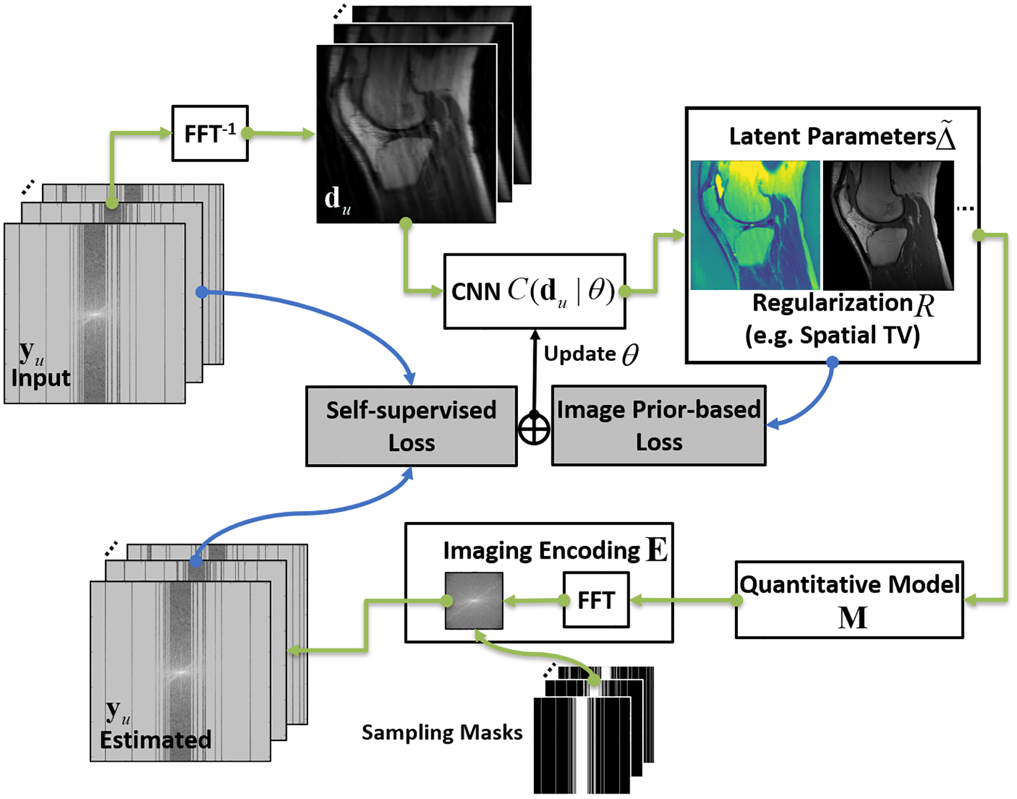
The schematic demonstration of the CNN framework implementing RELAX. A cyclic workflow was constructed to enforce self-supervised learning. The physics models and additional constraints can be incorporated into the framework to guide the learning of CNN mapping function to extract the latent image parameter maps from undersampled images. The labels follow the description in the main text.

METHODS

Quantitative MR Models

The RELAX framework was evaluated for reconstructing T1 and T2 maps from undersampled k-space data. T1 mapping was performed based on variable flip angle (VFA) imaging with a spoiled gradient echo sequence (27,28). The MR signal model for VFA imaging has an analytical solution at steady-state as follows (29):

$$\mathbf{M}=S_j\left({\text{I}}_0,{\text{T}}_1\right)={\text{I}}_0\cdot \frac{(1-e^{-TR/{\text{T}}_1})\text{sin}{\alpha }_j}{1-e^{-TR/{\text{T}}_1}\text{cos}{\alpha }_j}$$ [8]

where I₀ (proton density image) and T1 are to-be-estimated MR image/parameter and α_j denotes the j^th flip angle for acquiring MRI images S_j. T2 mapping was performed based on multi-echo spin-echo imaging (30), and corresponding MR signal model is given by:

$$\mathbf{M}=S_j\left({\text{I}}_0,{\text{T}}_2\right)={\text{I}}_0\cdot e^{-T{E}_j/{\text{T}}_2}$$ [9]

where I₀ and T2 are to-be-estimated MR image/parameter and TE_j denotes the j^th echo time. While a more complex form of models for T1/T2 mapping using these two sequences has been described by accounting for system imperfections such as field inhomogeneity, stimulated echo, slice excitation profile, partial volume contamination etc.(31–33), the simple forms are used in this study for demonstrating the initial feasibility of RELAX.

Image Datasets

Simulated Brain Datasets

Simulation studies were first performed to validate the RELAX framework. The BrainWeb (https://brainweb.bic.mni.mcgill.ca/) brain phantoms (34), made from 20 healthy adults with inter-subject anatomical variabilities, were used to simulate synthetic MRI datasets. Each brain phantom represents a 3D discrete tissue mask covering the whole brain for a total of eleven tissue types, including gray/white matter, cerebrospinal fluid, and connective tissues etc. These phantoms provided realistic brain structural features that were ideal for generating image datasets with brain anatomical information. The tissue relaxation parameters, including T₁, T₂ and I₀, were assigned to each voxel based on tissue type from previous literature (35,36). A realistic MR simulation system MRiLab (37) previously developed in our group was used to simulate MR signal acquisitions. MRiLab (https://leoliuf.github.io/MRiLab/) is an open-source MRI simulation system, which can simulate various pulse sequences given radiofrequency pulses, gradient waveforms, and acquisition schemes building on a discrete-time solution of the Bloch-equation by mean of rotation and exponential scaling matrices throughout the prescribed sequence (37–39). The simulated signal from all voxels in each phantom was then collected to fill an image matrix that forms ground truth k-space. It should be noted that our simulation directly generated fully sampled multi-contrast k-space by emulating a given MRI sequence. A schematic description of the simulation workflow is shown in Supporting Information Figure S1.

Fully sampled multi-contrast MRI k-space data were simulated using both the VFA spoiled gradient echo sequence and multi-echo spin-echo sequence. For VFA-based T1 mapping, the imaging parameters were: repetition time/echo times (TR/TE) = 8.5/3.9 ms, 8 flip angles = [3, 4, 5, 6, 7, 9, 13, 18]°, bandwidth = 326Hz/pixel, slice thickness = 3mm, number of slices = 40, field of view (FOV) = 22×22cm², and acquired image matrix = 256×256. For multi-echo spin-echo-based T2 mapping, the imaging parameters were: TR = 2500ms, 16 linear spacing TEs = [10, 20, 30, …, 160] ms, flip angle = 90°, bandwidth = 488Hz/pixel, slice thickness = 3mm, number of slices = 40, field of view (FOV) = 22×22cm², and acquired image matrix = 256×256. There was a total of 800 simulated image slices for all brain phantoms.

In-Vivo Knee Datasets

RELAX was further evaluated in in-vivo knee image datasets. This retrospective study was approved by the Institutional Review Board with a waiver of written informed consent. Data were acquired using the T1 mapping or T2 mapping sequences described above. For VFA T1 mapping, images of the knee were acquired in the sagittal plane for 50 symptomatic patients using a 3T GE scanner (MR 750, GE Healthcare, Waukesha, Wisconsin) and with an eight-channel phased-array knee coil (InVivo, Orlando, Florida). Relevant imaging parameters included: TR/TE = 4.6/2.2 ms, 8 flip angle = [3, 4, 5, 6, 7, 9, 13, 18]°, slice thickness = 3mm, pixel bandwidth = 122Hz/pixel, number of slices = 32, field of view = 16×16cm², and acquired image matrix = 256×256. No parallel imaging was used. The images were reconstructed on the MR scanner and were saved as DICOM files after coil combination. There was a total of 1600 image slices for all subjects. For multi-echo spin-echo T2 mapping, images were acquired in the sagittal plane for another 110 symptomatic patients using a 3T GE scanner (Signa Excite Hdx, GE Healthcare) and the same knee coil. Relevant imaging parameters included: 8 TEs/TR = [7, 16, 25, 34, 43, 52, 62, 71]/1500 ms, flip angle = 90°, slice thickness = 3–3.2mm, pixel bandwidth = 122Hz/pixel, number of slices = 18–20, field of view = 16×16cm², and acquired image matrix = 320×256. No parallel imaging was used. The images were reconstructed on the MR scanner and were saved as DICOM files after coil combination. There was a total of 2107 image slices for all subjects.

Experiment Design: Suppression of Noises and Undersampling Artifacts

The performance of RELAX was evaluated for suppressing image noises and/or aliasing artifacts induced by retrospectively undersampling MR k-space. Specifically, three experimental conditions were tested on the simulated brain T1 and T2 mapping datasets. The first experiment was designed to investigate the reconstruction accuracy and robustness of RELAX at various noise levels. The fully sampled k-space data were first normalized to a scale of 0–1. Complex Gaussian noise with an intensity of 0.025, 0.05, and 0.1 was then added into the simulated noise-free k-space to emulate noise contamination at different noise levels (2.5%, 5%, 10%). The noise was added to each frame of the multi-contrast images to ensure different noise characteristics across the multi-contrast parameter dimension.

The second experiment was designed to investigate the reconstruction performance of RELAX in accelerated images. Retrospective undersampling was performed to generate undersampled images by multiplying the fully sampled k-space data with undersampling masks followed by zero-filling reconstruction. The undersampling masks were generated based on a one-dimensional (phase-encoding dimension only) variable-density Cartesian random sampling pattern (40) to achieve an undersampling factor (R) of 5, and it had a fully sampled k-space center (5% of the total samples). The sampling pattern varied along the multi-contrast parameter dimension to create temporal incoherence as implemented in standard sparse image reconstruction. The third experiment was designed to investigate the reconstruction performance of RELAX in the condition of both noise and undersampling artifacts contaminations. For this, both complex Gaussian noise (noise level=5%) and 1D Cartesian undersampling (R=5) were applied to the simulated noise-free fully sampled k-space data to generate noisy images with undersampling artifacts.

In addition, to test its performance in different anatomy and validate its applicability in real MRI data, RELAX was also evaluated on fully sampled in-vivo knee T1 and T2 image datasets. Experiments were carried out to test the reconstruction performance of RELAX for rapid T1 and T2 mapping using retrospective undersampling, which was performed using the abovementioned one-dimensional variable-density sampling scheme at R=5.

To validate the reconstruction accuracy of RELAX, reference T1 and T2 maps were generated by fitting the fully-sampled simulated and in-vivo-acquired images using corresponding quantitative signal models described in Eq.[8] and Eq.[9] on a pixel-wise basis. The fitting was performed with a standard nonlinear least-squares (NLLS) algorithm. It should be noted that the reference images/parameter maps were not included in the training of RELAX.

Implementation and Training of Neural Network

Inspired by many deep learning studies for end-to-end image reconstruction (5,20,41) and our previous studies for rapid quantitative MRI (18,25,26), a customized residual U-Net (42) structure was selected to perform the mapping function to translate noisy and/or undersampled input images into desired parameter maps. The U-Net structure consisted of a paired encoder and decoder system, where the encoder aims to identify essential image features, remove uncorrelated structure and noise, and compress image information, while the decoder takes the output from encoder to form a targeted image contrast through a multi-level convolutional and combinational process. Symmetric shortcut connections were also created to directly transfer image features from the encoder to the decoder to augment the mapping efficiency. A modification of the U-Net is a residual learning design where an image by averaging all input images was directly subtracted from the estimated parameter maps. This residual learning has proven to be effective in several recent deep learning-based image reconstruction and synthesis studies (5,20,41). The detailed CNN structure is shown in Supporting Information Figure S2.

The image datasets were randomly split into 70%, 10% and 20% for training, validation and testing purposes, respectively. During the training step, a series of undersampled images for one slice were concatenated together and treated as a multi-channel 2D image input (analogous to the RGB channels in natural images) for the residual U-Net. The network parameters were initialized using the strategy described in (43). A standard mini-batch training was performed with each batch consisting of 3 slices for one iteration. The network parameters were updated using an adaptive gradient descent optimization (ADAM) algorithm (44) with a fixed learning rate of 0.0002 for total iteration steps corresponding to 200 epochs to ensure training convergence. The best model was selected as the one that provided the lowest loss value in the validation datasets. The training loss curves are shown in Supporting Information Figure S3. Following Eq.[7], a spatial TV regularization was applied to the estimated parameter maps and K was set to use ℓ₂ norm. A default weight factor λ in Eq.[7] was empirically optimized and set to be 0.01. The effect of λ on the reconstructed parameter maps was also evaluated by varying the value of λ from 0 to 0.1 and by comparing with the reference parameter maps. The deep learning algorithm was coded using the Python language and Keras (45) deep learning package with Tensorflow (46) computing backend. All training and evaluation were conducted on a personal computer hosting a Linux system and one NVIDIA GeForce RTX 2080Ti graphics card, which has 4352 CUDA cores and 11GB GDDR6 GPU RAM.

Comparison of Reconstruction Methods

The reconstruction performance of RELAX was compared with the other two reconstruction methods. One method is a constrained reconstruction technique using a combination of low-rank and spatial-temporal smoothness constraint, k-t SLR, representing the state-of-the-art conventional iterative reconstruction approach (47). This method was performed using the source code with its default parameter settings from the original developers in https://research.engineering.uiowa.edu/cbig/content/matlab-codes-k-t-slr. Another method is a supervised deep learning method, MANTIS (Model-Augmented Neural neTwork with Incoherent k-space Sampling), recently proposed to reconstruct undersampled MR images for rapid quantitative MRI (18). This method uses an end-to-end supervised learning strategy by comparing the directly estimated parameter maps from undersampled images with the reference parameter maps. It enforces a pixel-wise loss between the generated parameter map and reference parameter map. Quantitative metrics, including the normalized Root Mean Squared Error (nRMSE), the Structural SIMilarity index (SSIM) between the reconstructed quantitative maps and the reference maps were used to assess the difference of reconstruction errors among methods. The relative reduction of Tenengrad measure (48,49) between the reconstructed quantitative maps and the reference maps were used to assess the image sharpness. The Wilcoxon signed-rank test was used to demonstrate the method difference at a statistical significance level defined as a p-value smaller than 0.05.

RESULTS

Figure 2 shows representative T1 maps estimated using RELAX in one simulated brain dataset at three different experiment conditions, respectively. On the T1 maps generated by using the standard NLLS fitting, there is notable noise contamination caused by the added Gaussian noise at 5% noise level (NL) and aliasing artifacts caused by the k-space undersampling at R=5 with simple zero-filling reconstruction. RELAX successfully suppressed the noises and removed the undersampling artifacts through self-supervised deep learning reconstruction, providing image quality that is comparable to the noise/artifact-free ground truth (G.T.) T1 map. In the case with both noise contamination and undersampling artifacts, RELAX still managed to reconstruct the T1 map without observable residual artifact and noise amplification. These results demonstrated the ability of RELAX to model T1 mapping based on a VFA with a spoiled gradient echo sequence at imaging acceleration, increased noise or both.

Figure 2:

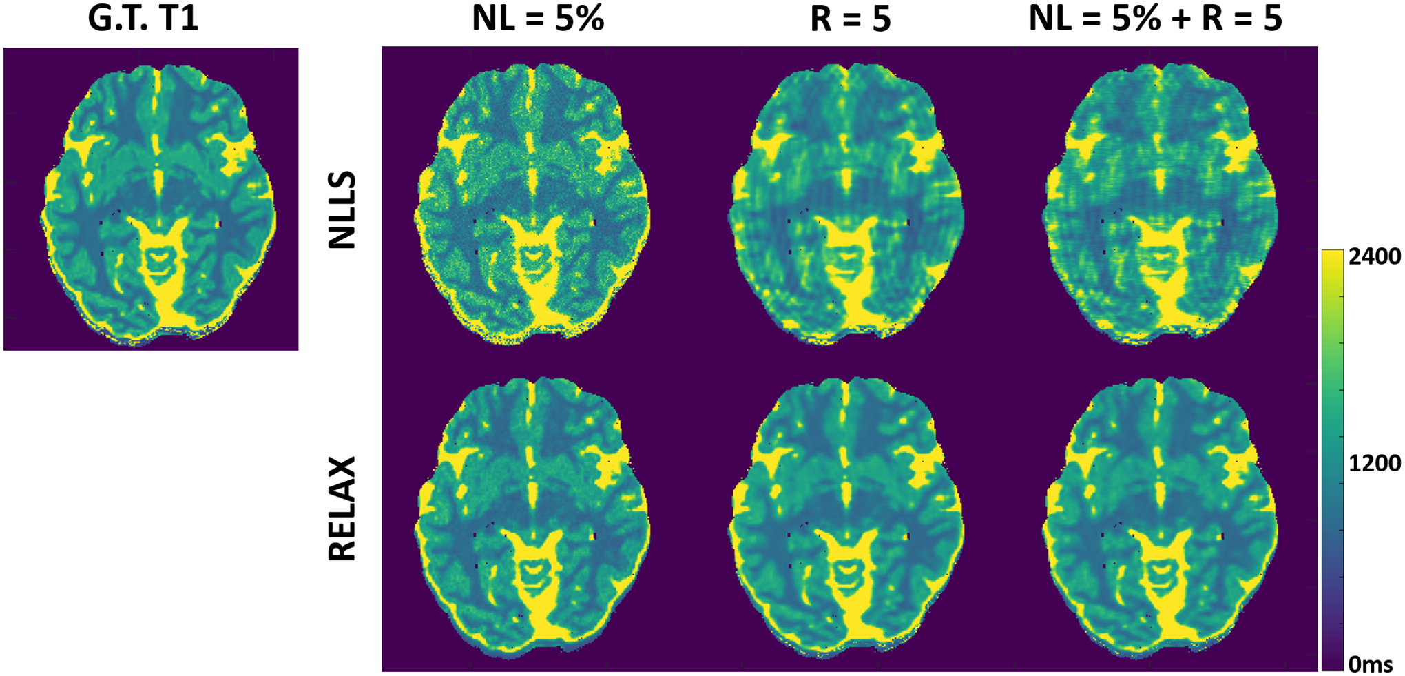
Representative T1 maps estimated using RELAX in one simulated brain dataset at three different experiment conditions, respectively. RELAX successfully suppressed the noises at 5% noise level (NL) and removed the undersampling artifacts at R=5 through self-supervised deep learning reconstruction, providing image quality that is comparable to the noise/artifact-free ground truth (G.T.) T1 map. The NLLS was applied to zero-filling reconstructed images at R=5.

Figure 3 shows representative T2 maps estimated using RELAX in another simulated brain dataset at three different experiment conditions, respectively. Similar to the T1 mapping experiments in Figure 2. RELAX enabled suppression of image noises and undersampling artifacts and reconstructed T2 maps that are comparable to the noise/artifact-free ground truth T2 maps. Figures 2 and 3 demonstrate the generality of RELAX to model different quantitative imaging process by incorporating corresponding signal models based on self-supervised learning.

Figure 3:

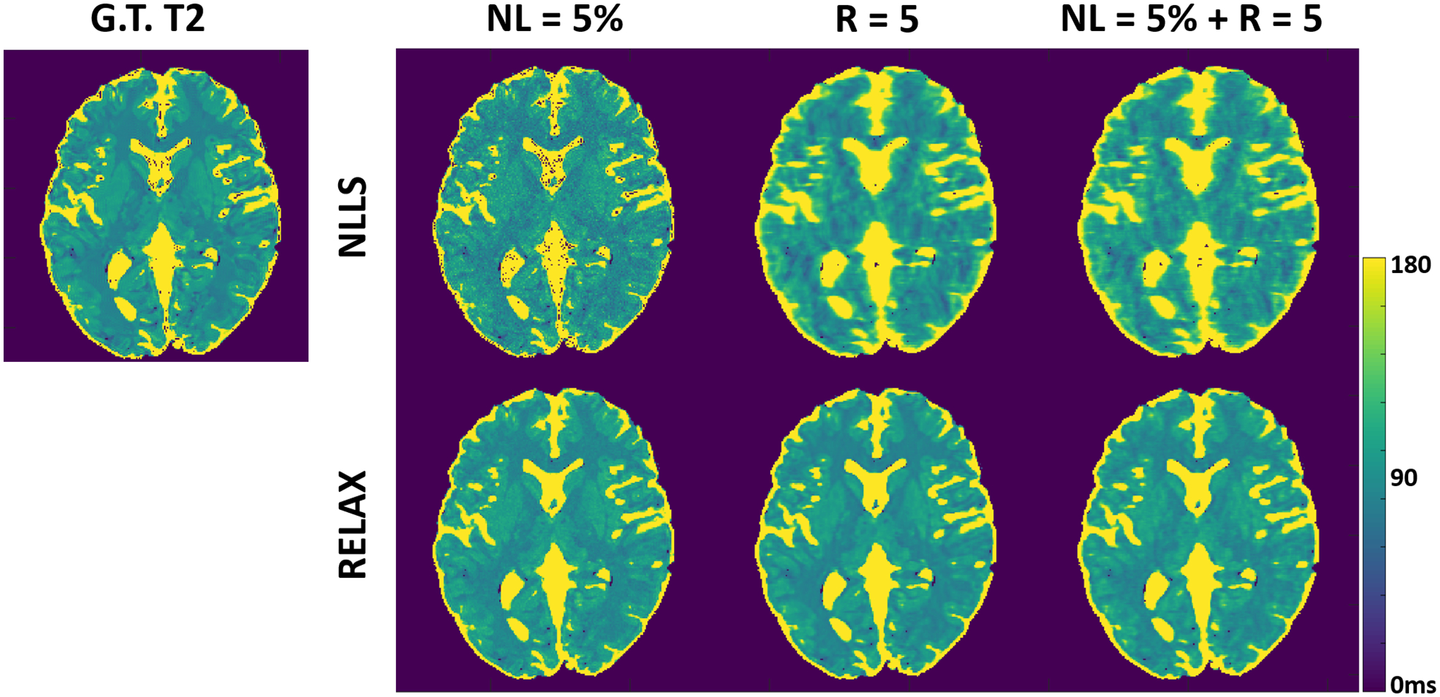
Representative T2 maps estimated using RELAX in one simulated brain dataset at three different experiment conditions, respectively. RELAX successfully suppressed the noises at 5% noise level (NL) and removed the undersampling artifacts at R=5 through self-supervised deep learning reconstruction, providing image quality that is comparable to the noise/artifact-free ground truth (G.T.) T2 map. The NLLS was applied to zero-filling reconstructed images at R=5.

The influence of the weighting parameter λ (for spatial TV constraint in this work) on reconstructed parameter maps is shown in Figure 4. While the self-supervised learning in RELAX has captured correct image features and contrast for gray/white matter after adequate training, certain noise appearance remains in images with self-supervision only (λ = 0). The inclusion of a spatial TV constraint further helped remove the residual noise and resulted in a cleaner tissue appearance at λ = 0.01. However, a stronger TV constraint (e.g., λ = 0.1) can lead to over smoothness on the parameter map and cause notable image blurring. As a result, proper selection of the weight for the additional regularization in RELAX has an apparent effect on the reconstructed quantitative maps.

Figure 4:

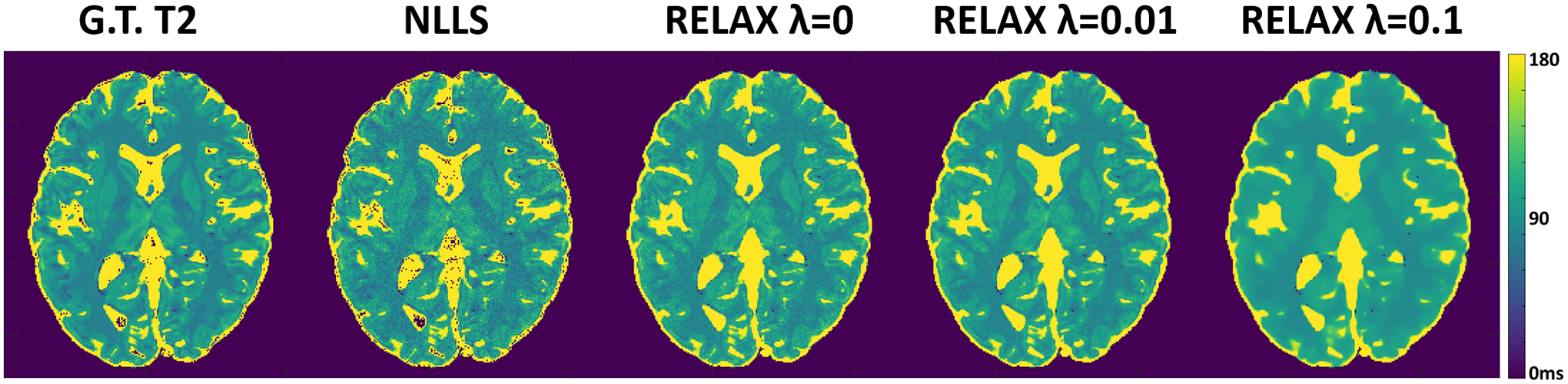
Examples showing the influence of the weighting parameter (for spatial TV constraint) on reconstructed parameter maps.

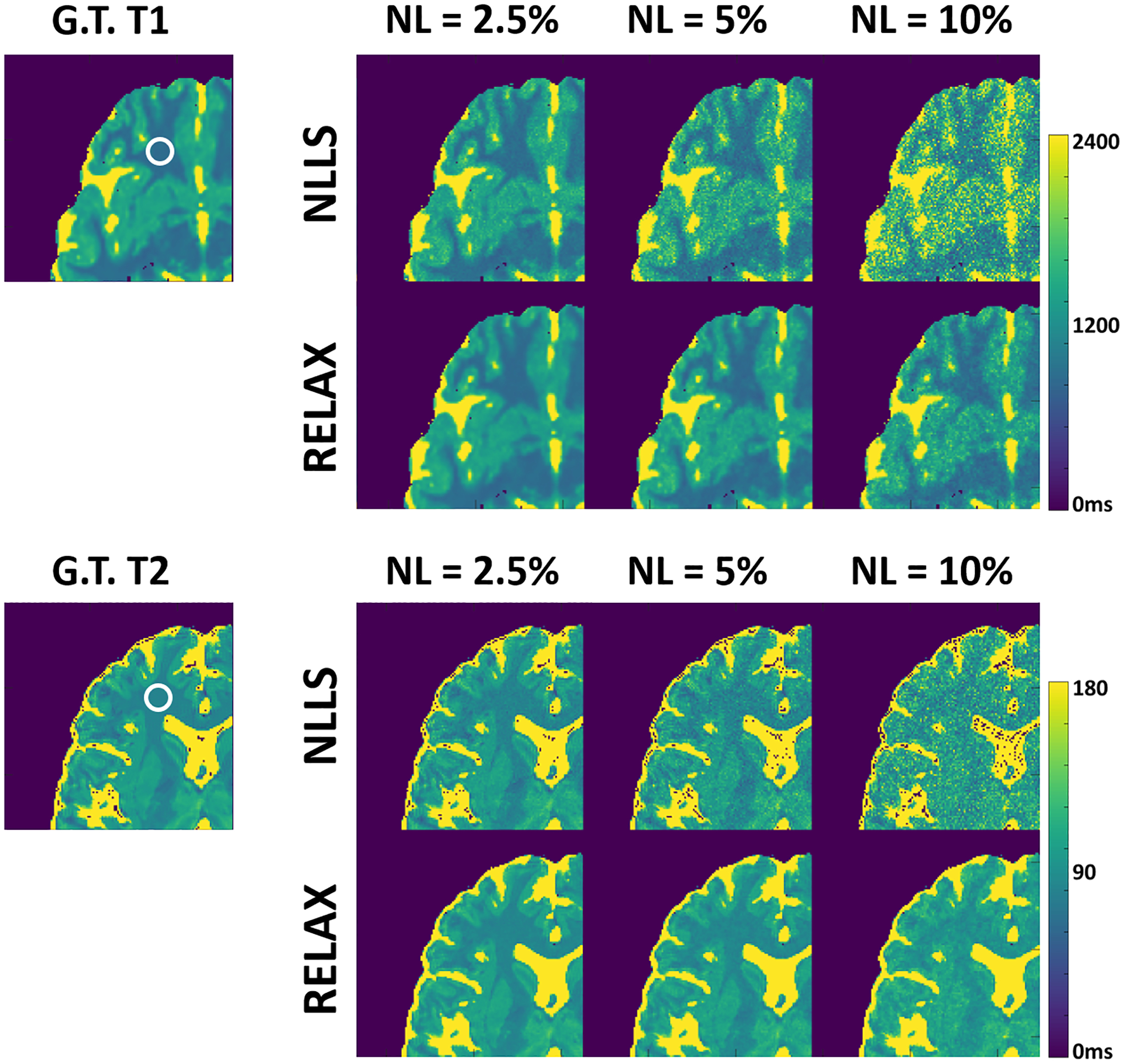
Figure 5 shows the performance of RELAX in different noise levels. Generally, RELAX generated acceptable T1 or T2 parameters at different noise conditions due to the inherent noise suppression in CNN training and the additional spatial TV constraint. An accurate T1 and T2 maps can be achieved at a low (NL=2.5%) and intermediate (NL=5%) noise level. At a high noise level (NL=10%) where the standard NLLS failed to provide reliable tissue differentiation, RELAX still managed to remove most of the noise and restore the essential image contrast between the grey matter, white matter, and cerebrospinal fluid in both T1 and T2 maps. In this example, the signal-to-noise ratio (SNR) was approximately 44, 26 and 14 in the circled white matter region on the 7° VFA image (for T1 mapping) at the noise level of 2.5%, 5% and 10%, respectively. The SNR was approximately 46, 23, 12 in the circled white matter region on the first echo image (for T2 mapping) at the noise level of 2.5%, 5% and 10%, respectively.

Figure 5:

Examples showing the performance of RELAX in different noise levels. RELAX generated acceptable T1 or T2 parameters at different noise conditions due to the inherent noise suppression in CNN training and the additional spatial TV constraint.

Figure 6 shows two representative slices of T1 maps estimated from different reconstruction methods for a testing knee dataset at R=5. Although k-t SLR was able to restore some image details by removing undersampling artifacts and sharpened the appearance, residual artifacts are noticed in T1 maps, particularly in the bone and muscle. The deep learning-based methods, including both MANTIS and RELAX, removed most of the artifacts and showed a similar reconstruction performance, although the MANTIS might have a closer appearance to the reference T1 maps due to its implementation of supervised learning. The RELAX reconstruction generated T1 maps with image quality that is comparable to the reference T1 maps obtained from fully sampled images. RELAX successfully removed almost all the image artifacts caused by k-space undersampling and provided a well-preserved image contrast, clarity, and tissue boundaries between cartilage, meniscus, and muscle highlighted in the zoom-in areas. There was also noticeable noise suppression in bone and muscle in the RELAX T1 maps. In this example, the SNR was approximately 48 in the cartilage region on the fully sampled 7° VFA image.

Figure 6:

Two representative slices of T1 maps estimated from different reconstruction methods for a testing knee dataset at R=5. The RELAX reconstruction generated T1 maps with image quality that is comparable to the reference T1 maps obtained from fully sampled images.

Figure 7 compares T1 maps generated from different reconstruction methods for another testing knee dataset at R=5. The absolute error map for each reconstructed T1 map was shown in the bottom, which also indicates better reconstruction accuracy for both MANTIS and RELAX methods in comparison to conventional constrained reconstruction.

Figure 7:

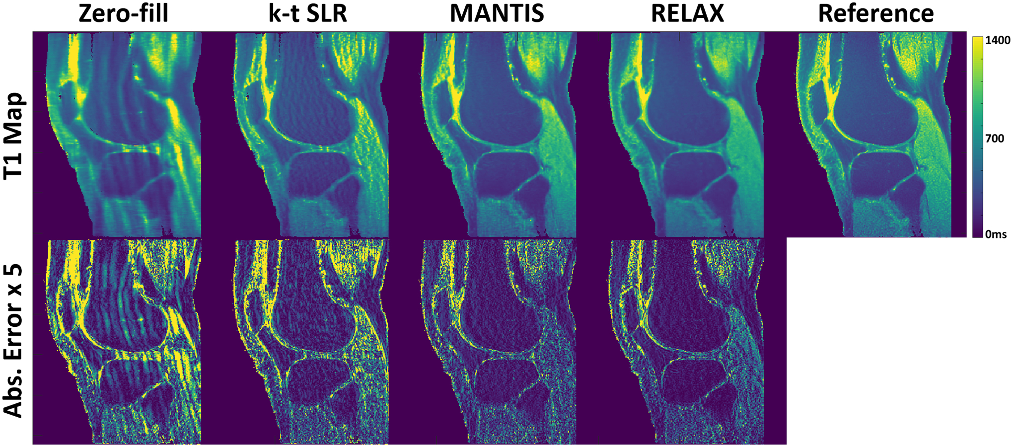
Comparison of T1 maps generated from different reconstruction methods for another testing knee dataset at R=5. The deep learning-based methods, including both MANTIS and RELAX, removed most of the artifacts and showed a similar reconstruction performance, which outperformed conventional constrained reconstruction k-t SLR. The absolute error maps were amplified by five times for display purposes to show the method difference.

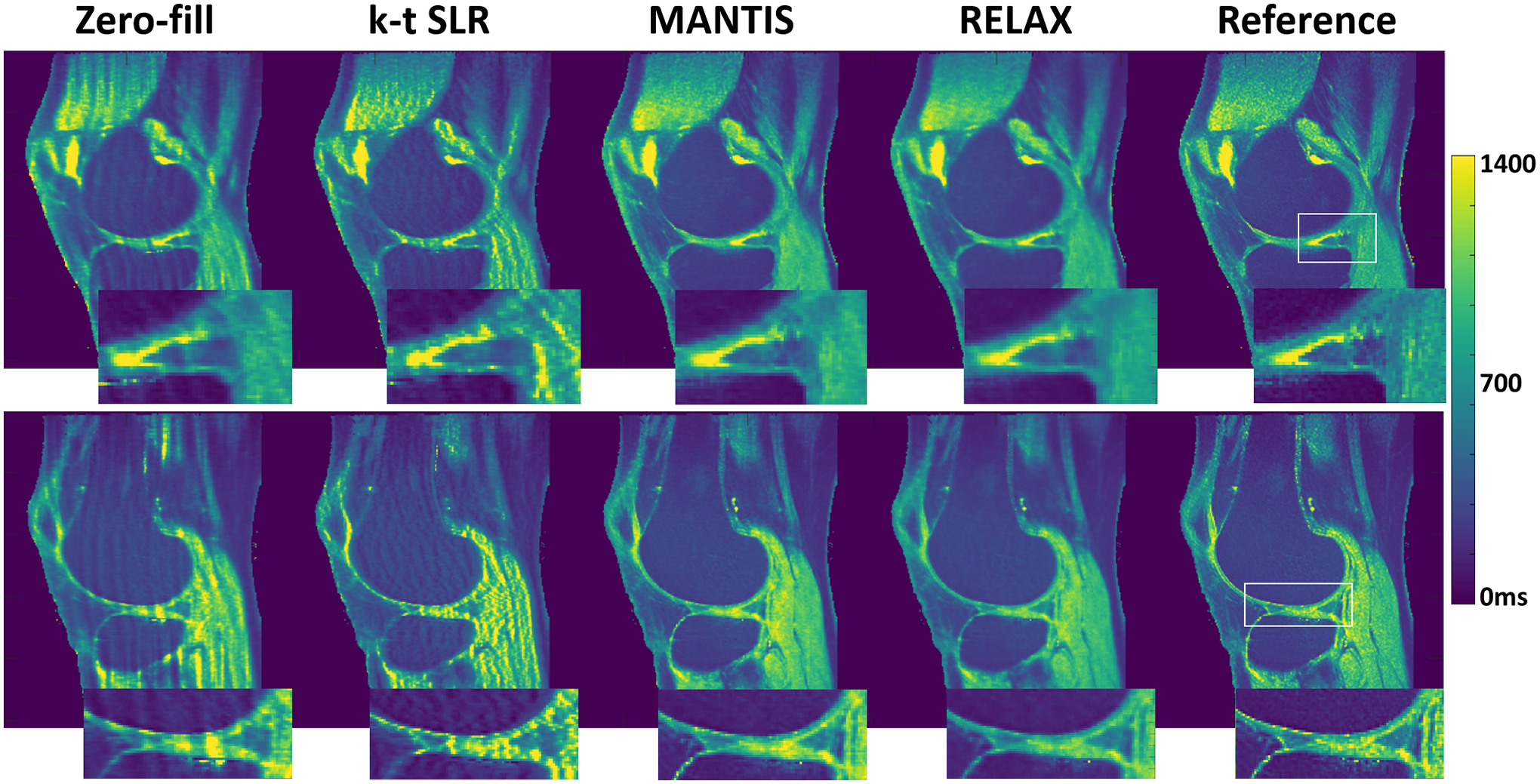
Figure 8 shows two representative slices of T2 maps estimated from different reconstruction methods for a testing knee dataset at R=5. Similar to that in T1 mapping, both MANTIS and RELAX provided nearly artifact-free T2 maps and presented similar reconstruction performance. RELAX generated T2 maps with successful suppression of image artifacts and noise compared to the reference T2 maps obtained from fully sampled images. RELAX also provided well-preserved image contrast and tissue details highlighted in the zoom-in areas. There was also noticeable noise suppression but slight image blurring in the bone and muscle in the T2 maps generated from RELAX, in contrast to the MANTIS result and the reference T2 map. In this example, the SNR was approximately 79 in the cartilage region on the fully sampled first echo image.

Figure 8:

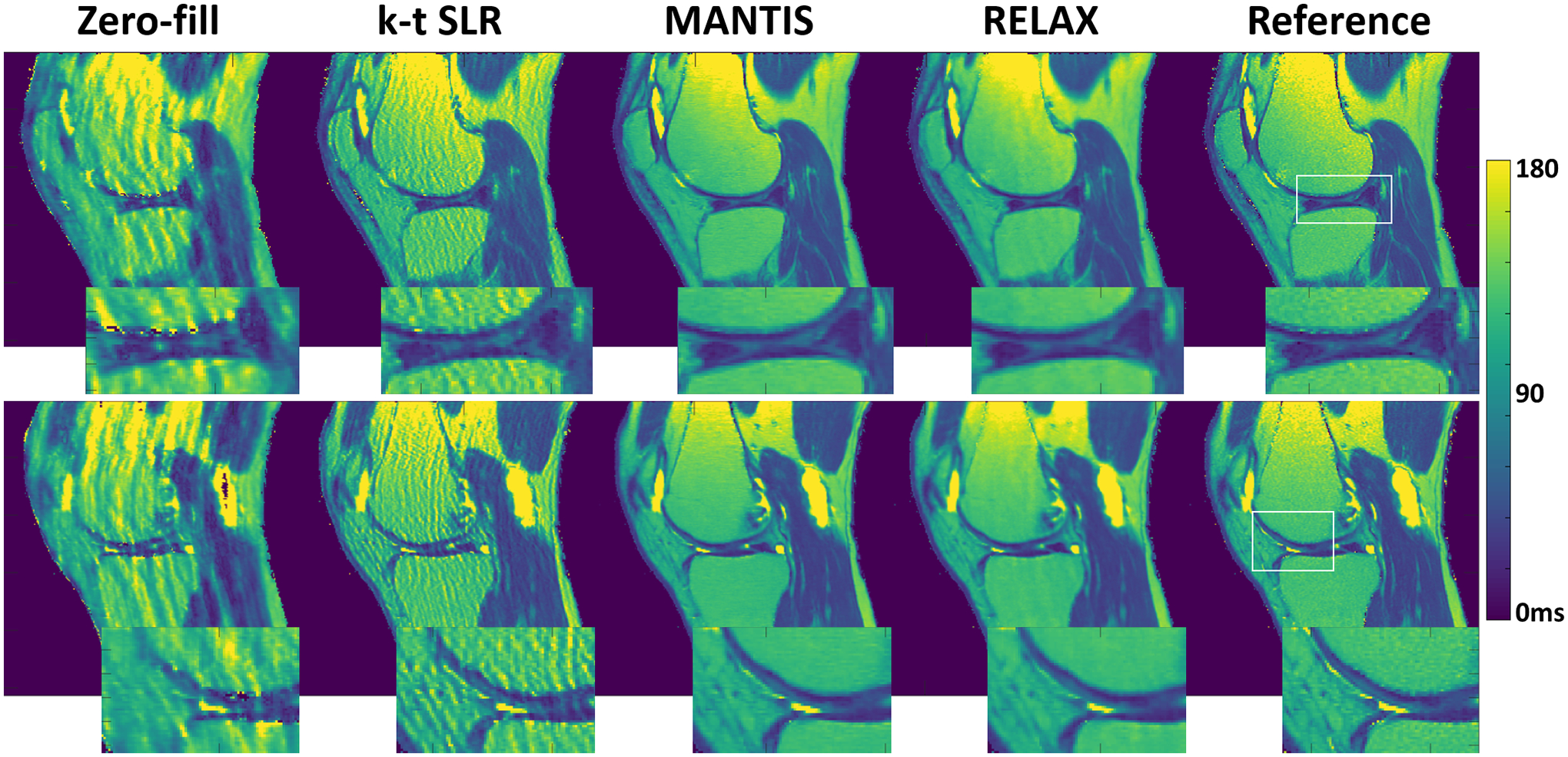
Two representative slices of T2 maps estimated from different reconstruction methods for a testing knee dataset at R=5. RELAX generated T2 maps with successful suppression of image artifacts and noise compared to the reference T2 maps obtained from fully sampled images. There was noticeable noise suppression but a slight image blurring in the bone and muscle in the T2 maps generated from RELAX. To better highlight cartilage contrast, the same example with an adjusted color window was also provided in the Supporting Information Figure S4.

Figure 9 compares T2 maps generated from different reconstruction methods for another testing knee dataset at R=5. The absolute error map for each reconstructed T2 map indicated better reconstruction accuracy for both MANTIS and RELAX in comparison to k-t SLR in terms of artifact removal and image contrast preservation.

Figure 9:

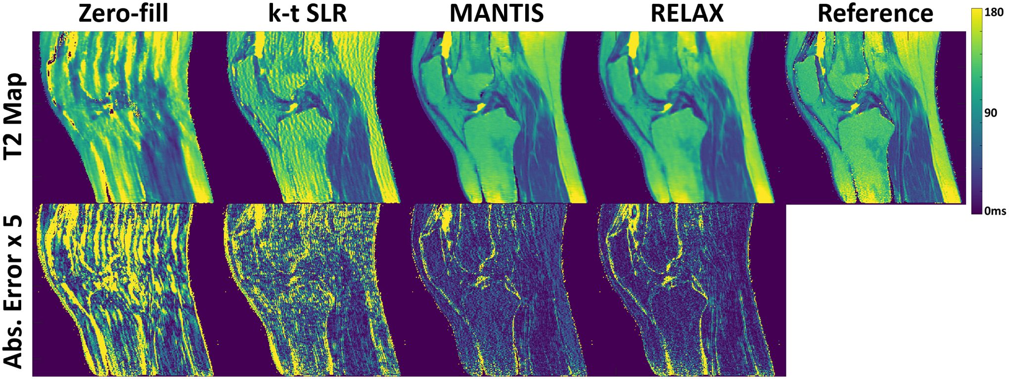
Comparison of T2 maps generated from different reconstruction methods for another testing knee dataset at R=5. Both MANTIS and RELAX provided nearly artifact-free T2 maps and presented similar reconstruction performance. The absolute error map for each reconstructed T2 map indicated better reconstruction accuracy for both MANTIS and RELAX in comparison to k-t SLR. The absolute error maps were amplified by five times for display purposes to show the method difference.

Finally, qualitative comparison was further validated by quantitative metrics. As shown in Table 1, both RELAX and MANTIS achieved significantly better reconstruction performance (all p<0.001) than k-t SLR in terms of reconstruction errors and image sharpness and texture preservation for both T1 and T2 mapping. The results between RELAX and MANTIS were comparable, while the supervised learning method MANTIS yielded better image sharpness as indicated by the lower Tenengrad measures (p=0.019 for T1 and for p<0.001 T2) and better overall image feature preservation as indicated by the higher SSIM measures (p<0.001 for T1 and for p<0.001 T2). RELAX achieved better noise suppression than MANTIS as indicated by the lower nRMSE measures (p=0.001 for T1 and for p=0.02 for T2). In addition, quantitative comparison of the mean T1 and T2 values from the cartilage between RELAX and the references was also assessed using the Bland-Altman analysis (50) in Supporting Information Figure S5. A comparison between the performance of RELAX using residual U-Net and that using the standard U-Net without residual learning was provided in Supporting Information Table S1.

Table 1:

nRMSE, SSIM, and Tenengrad measures between the reference quantitative maps estimated from the fully sampled images and the reconstructed quantitative maps estimated using different methods at an acceleration rate R=5. Results were shown as the mean and standard deviation (SD) values over the testing datasets for knee images for VFA T1 mapping and multi-echo spin-echo T2 mapping, respectively. MANTIS and RELAX achieved better reconstruction performance than the k-t SLR method. MANTIS had the highest image sharpness (i.e., lowest Tenengrad measures) and best texture preservation (i.e., highest SSIM measures) in comparison with all other methods. RELAX achieved the greatest noise suppression (i.e., lowest nRMSE measures).

Methods	Mean ± SD for T1 maps			Mean ± SD for T2 maps
	nRMSE (%)	SSIM (%)	Tenengrad (%)	nRMSE (%)	SSIM (%)	Tenengrad (%)
Zero-fill	13.3 ± 4.1	53.2 ± 8.3	37.4 ± 5.8	18.7 ± 3.4	48.2 ± 7.1	49.7 ± 9.7
k-t SLR	7.1 ± 2.7	76.4 ± 3.1	16.6 ± 5.3	10.9 ± 2.1	72.8 ± 5.8	18.3 ± 2.4
MANTIS	5.2 ± 2.1	87.3 ± 1.4	11.6 ± 2.1	6.4 ± 1.6	85.1 ± 2.2	9.9 ± 2.9
RELAX	5.0 ± 1.7	84.6 ± 2.5	13.2 ± 2.3	6.3 ± 1.3	82.4 ± 2.7	11.9 ± 2.5

DISCUSSION

This work proposed a model-guided self-supervised deep learning reconstruction technique towards rapid quantitative MR parameter mapping. We have demonstrated that by enforcing MRI physical model constraints, deep learning-based MRI reconstruction may be performed without fully sampled training references. The initial feasibility of using RELAX for accelerated T1 or T2 mapping was tested in both simulated MRI data where noise/artifact-free ground truth images are available and actually-acquired MRI data where fully sampled references are available. Our initial results have supported that RELAX can generate T1 or T2 maps that are comparable to T1/T2 maps from standard supervised learning and superior to T1/T2 maps from conventional constrained reconstruction.

There has been an explosive growth of deep learning-based MRI reconstruction works in the past few years, which have shown great potentials in overcoming several challenges that are presented in conventional constrained reconstruction, such as slow reconstruction speed and compromised reconstruction performance due to generic constraints (1–3,5,19–24). However, to date, most of these works have been focusing on supervised learning in which reference training datasets must be provided to guide network learning. While many deep learning architectures have shown the ability to learn sophisticated image features and patterns that are useful to represent essential image content in MRI reconstruction (2,4,6), it is observed that this purely data-driven approach could be compromised with limited training datasets, or in the presence of data discrepancy between training and testing datasets (5,18,51). In addition, ideal fully sampled MR images can often be challenging to acquire, for example, due to subject motion in dynamic MRI, contrast variation in contrast-enhanced MRI, or high noise contamination in low field MRI. Several prior works have shown that MR imaging model (e.g., Fourier encoding and coil encoding) can be embedded in network training to improve training performance (1,3,5,22–24). The incorporation of MR physics further regularizes the learning process and is proven to lead to efficient and robust reconstruction at a lower requirement for training datasets. Recent works have also proposed the new concept of self-supervised learning for MRI reconstruction (10,11). An early study has shown a denoising deep learning network can be successfully trained using pairs of noisy images (7). Self-supervised learning relies on a hypothesis that image noise and artifacts are typically incoherent in training data pairs, thus minimizing a loss between them readily regularizes the learning to capture coherent image content. A direct benefit of self-supervised learning is training without fully sampled reference, which can potentially facilitate image applications where ideal high-quality reference images are unavailable. Building on this theoretical foundation and the recent success of model-based and self-supervised learning, we proposed and evaluated RELAX by leveraging a combination of MR imaging model and a quantitative model to regularize network training with self-supervised learning. These physical models have been proven to jointly guide deep neural networks to generate accurate MR parameter maps while removing undersampling-induced artifacts and noises (18).

In addition, we also showed that additional sparsity constraints could be optionally added in RELAX framework to impose prior knowledge into the learning process. For example, we have demonstrated that a spatial TV constraint can be directly enforced on the MR parameter maps to be reconstructed to help improve reconstruction quality by suppressing residual noise/artifacts. The spatial TV constraint also proves to promote the smoothness of the generated parameter maps in deep learning, similar to that in conventional constrained reconstruction (52). However, it should be noted that an appropriate selection of corresponding regularization parameter, as shown in Eq.[7] is critical. Higher weighting for the spatial TV constraint tends to generate over-smoothness for parameter maps, as shown in Figure 4, as previously observed in conventional constrained reconstruction. Depending on the assumption for the to-be-reconstructed parameter maps, other prior knowledge-based constraints can also be imposed during the deep learning training process. For example, a combination of wavelet and spatial TV constraints, as used in compressed sensing reconstruction (40), can be applied to RELAX to improve regularization performance. Moreover, more advanced constraints, such as the total generalized variation (TGV) constraint (53) or low-rankness subspace modeling (54), can also be further considered to overcome the problem of simple TV constraint and to improve reconstruction performance. The incorporation of these physical constraints into deep learning opens a new approach to integrate physics-informed features into the learning process. However, similar to conventional constrained reconstruction, the regularization parameters are likely to influence the final reconstruction performance, and thus, they are subject to careful optimization. Future research for developing the strategy of comprehensive regularization parameter optimization is needed to validate the optimized performance of the network and the sensitivity of reconstruction results to these parameters. Adaptive and dataset-specific optimization of these parameters would also be a future research direction to create more generalizable deep learning models.

In this work, we have demonstrated the performance of RELAX for accelerated T1 or T2 mapping, respectively, based two different acquisition schemes. The VFA imaging using a spoiled gradient echo sequence is commonly used for rapid T1 mapping. While the Eq. [8] has an analytical description for MR signal at steady-state given different excitation flip angles, the T1 mapping can sometimes be more complicated due to B1 field inhomogeneity, imperfect slice profile, or transient state-steady (29). For example, an inversion recovery spoiled gradient echo acquisition can be added into the VFA to help correct the B1 effect (31). Likewise, T2 mapping using a multi-echo spin-echo sequence can be affected by several confounding factors, including B1 field inhomogeneity, excitation pulse profile, and stimulated echoes (33). While quantitative T1/T2 models using classic MR signal equations were used to prove the feasibility of RELAX in our study, it is anticipated that RELAX can be further improved with more comprehensive signal modeling in using advanced MR sequences and modeling. One recent study has shown that additional B1 field estimation can improve T1 mapping using a deep learning approach (55). Another study has also shown a joint estimation of T1 in the rotating frame (T1ρ) and T2 maps from undersampled images at a T1ρ and T2 preparation sequence is feasible using deep learning end-to-end mapping (56). Moreover, RELAX could also use a Bloch simulation-based signal model instead of an analytical model to capture more complex MR signal evolution, similar to that implemented in MR Fingerprinting (MRF) (57). The recent advance of deep learning-based MRF has laid a promising foundation to build a more efficient dictionary (58), to better capture spatiotemporal image features (59), and to generate MR signals much faster using a fully connected network than the standard dictionary matching (60). Finally, the RELAX framework is expected to be generalizable to other quantitative MRI applications by replacing the T1/T2 models with other quantitative models. Examples of these applications include diffusion MRI or quantitative susceptibility mapping (QSM), which may both benefit from the RELAX framework.

This study has several limitations that require further improvement. First, the performance of RELAX was only demonstrated on simulated and coil-combined real MRI datasets. The extension of RELAX to multiple coil acquisitions is expected to be straightforward by incorporating pre-estimated coil sensitivity maps. This extension may also impose a more definite model constraint by including Fourier encoding, coil encoding, and a quantitative imaging model for further improving reconstruction performance. It would be ideal to train the model using true multi-coil k-space data directly saved from MR scanner. The extension of RELAX to use raw multi-coil data is entirely possible and warranted given that appropriate and adequate multi-coil training dataset, better GPU architecture, and increased GPU memory are made available. Moreover, RELAX could also be combined with non-Cartesian sampling schemes, so that, for example, it can be applied for imaging moving organs to take advantage of the motion robustness provide by radial sampling(61,62). Second, we used a simple T1 and T2 model for demonstration purposes by considering only T1 relaxation and exponential T2 decaying. In practice, quantitative signal evolution is often contaminated by system imperfections that need to be accounted for in the future. These may be further incorporated into the training process as long as the unwanted issues associated with these system imperfections can be modeled. Third, the current study used a residual U-Net structure and did not compare the U-Net type with other end-to-end CNN mapping structures. It would be interesting to compare the U-Net with other newly developed deep learning networks to evaluate their performance in the RELAX framework. Finally, this current study has a relatively small number of subjects for training and testing. Further investigation for the performance of RELAX in a large scale clinical database and comprehensive radiologist evaluation is warranted to fully evaluate the sensitivity, repeatability, and robustness of our technique towards various pathologies.

CONCLUSIONS

This work has demonstrated the initial feasibility of RELAX for rapid quantitative MR parameter mapping based on self-supervised deep learning. This new technique may be particularly useful in quantitative MRI applications where fully sampled reference images are challenging to acquire. It holds great potential to improve imaging speed in quantitative MRI and to help the clinical translation of quantitative imaging.

REFERENCES

- 1.Hammernik K, Klatzer T, Kobler E, et al. Learning a Variational Network for Reconstruction of Accelerated MRI Data. Magn. Reson. Med 2017;79:3055–3071 doi: 10.1002/mrm.26977. [DOI] [PMC free article] [PubMed] [Google Scholar]
- 2.Akçakaya M, Moeller S, Weingärtner S, Uğurbil K. Scan-specific robust artificial-neural-networks for k-space interpolation (RAKI) reconstruction: Database-free deep learning for fast imaging. Magn. Reson. Med 2019;81:439–453 doi: 10.1002/mrm.27420. [DOI] [PMC free article] [PubMed] [Google Scholar]
- 3.Eo T, Jun Y, Kim T, Jang J, Lee HJ, Hwang D. KIKI-net: Cross-domain convolutional neural networks for reconstructing undersampled magnetic resonance images. Magn. Reson. Med 2018;80:2188–2201 doi: 10.1002/mrm.27201. [DOI] [PubMed] [Google Scholar]
- 4.Mardani M, Gong E, Cheng JY, et al. Deep Generative Adversarial Neural Networks for Compressive Sensing MRI. IEEE Trans. Med. Imaging 2019;38:167–179 doi: 10.1109/TMI.2018.2858752. [DOI] [PMC free article] [PubMed] [Google Scholar]
- 5.Liu F, Samsonov A, Chen L, Kijowski R, Feng L. SANTIS: Sampling-Augmented Neural neTwork with Incoherent Structure for MR image reconstruction. Magn. Reson. Med 2019;82:1890–1904 doi: 10.1002/mrm.27827. [DOI] [PMC free article] [PubMed] [Google Scholar]
- 6.LeCun Y, Bengio Y, Hinton G. Deep learning. Nature 2015;521:436–444 doi: 10.1038/nature14539. [DOI] [PubMed] [Google Scholar]
- 7.Lehtinen J, Munkberg J, Hasselgren J, et al. Noise2Noise: Learning Image Restoration without Clean Data. 35th Int. Conf. Mach. Learn. ICML 2018 2018;7:4620–4631. [Google Scholar]
- 8.Tamir JI, Yu SX, Lustig M. Unsupervised Deep Basis Pursuit: Learning Reconstruction without Ground-Truth Data. In: Proc Intl Soc Mag Reson Med.; 2019. [Google Scholar]
- 9.Huang P, Zhang C, Li H, et al. Deep MRI Reconstruction without Ground Truth for Training. In: Proc Intl Soc Mag Reson Med.; 2019. [Google Scholar]
- 10.Senouf O, Vedula S, Weiss T, Bronstein A, Michailovich O, Zibulevsky M. Self-supervised learning of inverse problem solvers in medical imaging. In: Lecture Notes in Computer Science (including subseries Lecture Notes in Artificial Intelligence and Lecture Notes in Bioinformatics). Vol. 11795 LNCS. Springer; 2019. pp. 111–119. doi: 10.1007/978-3-030-33391-1_13. [DOI] [Google Scholar]
- 11.Yaman B, Hosseini SAH, Moeller S, Ellermann J, Uğurbil K, Akçakaya M. Self-supervised learning of physics-guided reconstruction neural networks without fully sampled reference data. Magn. Reson. Med 2020:1–20 doi: 10.1002/mrm.28378. [DOI] [PMC free article] [PubMed] [Google Scholar]
- 12.Liu J, Sun Y, Eldeniz C, Gan W, An H, Kamilov US. RARE: Image Reconstruction using Deep Priors Learned without Ground Truth. IEEE J. Sel. Top. Signal Process 2020:1–1 doi: 10.1109/jstsp.2020.2998402. [DOI] [Google Scholar]
- 13.Block KTKT, Uecker M, Frahm J. Model-Based Iterative Reconstruction for Radial Fast Spin-Echo MRI. IEEE Trans. Med. Imaging 2009;28:1759–1769 doi: 10.1109/TMI.2009.2023119. [DOI] [PubMed] [Google Scholar]
- 14.Wang X, Roeloffs V, Klosowski J, et al. Model-based T1 mapping with sparsity constraints using single-shot inversion-recovery radial FLASH. Magn. Reson. Med 2018;79:730–740 doi: 10.1002/mrm.26726. [DOI] [PubMed] [Google Scholar]
- 15.Fessler J Model-Based Image Reconstruction for MRI. IEEE Signal Process. Mag 2010;27:81–89 doi: 10.1109/MSP.2010.936726. [DOI] [PMC free article] [PubMed] [Google Scholar]
- 16.Sumpf TJ, Uecker M, Boretius S, Frahm J. Model-based nonlinear inverse reconstruction for T2 mapping using highly undersampled spin-echo MRI. J. Magn. Reson. Imaging 2011;34:420–428 doi: 10.1002/jmri.22634. [DOI] [PubMed] [Google Scholar]
- 17.Knoll F, Raya JG, Halloran RO, et al. A model-based reconstruction for undersampled radial spin-echo DTI with variational penalties on the diffusion tensor. NMR Biomed. 2015;28:353–366 doi: 10.1002/nbm.3258. [DOI] [PMC free article] [PubMed] [Google Scholar]
- 18.Liu F, Feng L, Kijowski R. MANTIS: Model-Augmented Neural neTwork with Incoherent k-space Sampling for efficient MR parameter mapping. Magn. Reson. Med 2019;82:174–188 doi: 10.1002/mrm.27707. [DOI] [PMC free article] [PubMed] [Google Scholar]
- 19.Wang S, Su Z, Ying L, et al. Accelerating Magnetic Resonance Imaging Via Deep Learning. In: 2016 IEEE 13th International Symposium on Biomedical Imaging (ISBI). IEEE; 2016. pp. 514–517. doi: 10.1109/ISBI.2016.7493320. [DOI] [PMC free article] [PubMed] [Google Scholar]
- 20.Han Y, Yoo J, Kim HH, Shin HJ, Sung K, Ye JC. Deep learning with domain adaptation for accelerated projection-reconstruction MR. Magn. Reson. Med 2018;80:1189–1205 doi: 10.1002/mrm.27106. [DOI] [PubMed] [Google Scholar]
- 21.Zhu B, Liu JZ, Cauley SF, Rosen BR, Rosen MS. Image reconstruction by domain-transform manifold learning. Nature 2018;555:487–492 doi: 10.1038/nature25988. [DOI] [PubMed] [Google Scholar]
- 22.Schlemper J, Caballero J, Hajnal JV, Price AN, Rueckert D. A Deep Cascade of Convolutional Neural Networks for Dynamic MR Image Reconstruction. IEEE Trans. Med. Imaging 2018;37:491–503 doi: 10.1109/TMI.2017.2760978. [DOI] [PubMed] [Google Scholar]
- 23.Biswas S, Aggarwal HK, Jacob M. Dynamic MRI using model-based deep learning and SToRM priors: MoDL-SToRM. Magn. Reson. Med 2019. doi: 10.1002/mrm.27706. [DOI] [PMC free article] [PubMed] [Google Scholar]
- 24.Malavé MO, Baron CA, Koundinyan SP, et al. Reconstruction of undersampled 3D non-Cartesian image-based navigators for coronary MRA using an unrolled deep learning model. Magn. Reson. Med 2020;84:800–812 doi: 10.1002/mrm.28177. [DOI] [PMC free article] [PubMed] [Google Scholar]
- 25.Zha W, Fain SB, Kijowski R, Liu F. Relax-MANTIS: REference-free LAtent map-eXtracting MANTIS for efficient MR parametric mapping with unsupervised deep learning. In: Proc Intl Soc Mag Reson Med.; 2019. [Google Scholar]
- 26.Liu F, Feng L. Towards High-Performance Rapid Quantitative Imaging via Model-based Deep Adversarial Learning. In: ISMRM Workshop on Data Sampling & Image Reconstruction.; 2020. [Google Scholar]
- 27.Wang HZ, Riederer SJ, Lee JN. Optimizing the precision in T1 relaxation estimation using limited flip angles. Magn. Reson. Med 1987;5:399–416 doi: 10.1002/mrm.1910050502. [DOI] [PubMed] [Google Scholar]
- 28.Venkatesan R, Lin W, Haacke EM. Accurate determination of spin-density and T1 in the presence of RF- field inhomogeneities and flip-angle miscalibration. Magn. Reson. Med 1998;40:592–602 doi: 10.1002/mrm.1910400412. [DOI] [PubMed] [Google Scholar]
- 29.Stikov N, Boudreau M, Levesque IR, Tardif CL, Barral JK, Pike GB. On the accuracy of T1 mapping: Searching for common ground. Magn. Reson. Med 2015;73:514–522 doi: 10.1002/mrm.25135. [DOI] [PubMed] [Google Scholar]
- 30.Meiboom S, Gill D. Modified Spin-Echo Method for Measuring Nuclear Relaxation Times. Rev. Sci. Instrum 1958;29:688–691 doi: 10.1063/1.1716296. [DOI] [Google Scholar]
- 31.Deoni SCL. High-resolution T1 mapping of the brain at 3T with driven equilibrium single pulse observation of T1 with high-speed incorporation of RF field inhomogeneities (DESPOT1-HIFI). J Magn Reson Imaging 2007;26:1106–1111 doi: 10.1002/jmri.21130. [DOI] [PubMed] [Google Scholar]
- 32.Deoni SC, Rutt BK, Arun T, Pierpaoli C, Jones DK. Gleaning multicomponent T1 and T2 information from steady-state imaging data. Magn Reson Med 2008;60:1372–1387 doi: 10.1002/mrm.21704. [DOI] [PubMed] [Google Scholar]
- 33.Ben-Eliezer N, Sodickson DK, Block KT. Rapid and accurate T2 mapping from multi-spin-echo data using bloch-simulation-based reconstruction. Magn. Reson. Med 2015;73:809–817 doi: 10.1002/mrm.25156. [DOI] [PMC free article] [PubMed] [Google Scholar]
- 34.Aubert-Broche B, Griffin M, Pike GB, Evans AC, Collins DL. Twenty new digital brain phantoms for creation of validation image data bases. IEEE Trans. Med. Imaging 2006;25:1410–1416 doi: 10.1109/TMI.2006.883453. [DOI] [PubMed] [Google Scholar]
- 35.Stanisz GJ, Odrobina EE, Pun J, et al. T1, T2 relaxation and magnetization transfer in tissue at 3T. Magn Reson Med 2005;54:507–512 doi: 10.1002/mrm.20605. [DOI] [PubMed] [Google Scholar]
- 36.Brown RW, Cheng YCN, Haacke EM, Thompson MR, Venkatesan R. Magnetic Resonance Imaging: Physical Principles and Sequence Design: Second Edition. (Brown RW, Cheng Y-CN, Haacke EM, Thompson MR, Venkatesan R, editors.) Chichester, UK: Wiley Blackwell; 2014. doi: 10.1002/9781118633953. [DOI] [Google Scholar]
- 37.Liu F, Velikina JV, Block WF, Kijowski R, Samsonov AA. Fast Realistic MRI Simulations Based on Generalized Multi-Pool Exchange Tissue Model. IEEE Trans. Med. Imaging 2017;36:527–537 doi: 10.1109/TMI.2016.2620961. [DOI] [PMC free article] [PubMed] [Google Scholar]
- 38.Bittoun J, Taquin J, Sauzade M. A computer algorithm for the simulation of any nuclear magnetic resonance (NMR) imaging method. Magn Reson Imaging 1984;2:113–120. [DOI] [PubMed] [Google Scholar]
- 39.Benoit-Cattin H, Collewet G, Belaroussi B, Saint-Jalmes H, Odet C. The SIMRI project: a versatile and interactive MRI simulator. J. Magn. Reson 2005;173:97–115 doi: 10.1016/j.jmr.2004.09.027. [DOI] [PubMed] [Google Scholar]
- 40.Lustig M, Donoho D, Pauly JM. Sparse MRI: The application of compressed sensing for rapid MR imaging. Magn Reson Med 2007;58:1182–1195 doi: 10.1002/mrm.21391. [DOI] [PubMed] [Google Scholar]
- 41.Gong E, Pauly JM, Wintermark M, Zaharchuk G. Deep learning enables reduced gadolinium dose for contrast-enhanced brain MRI. J. Magn. Reson. Imaging 2018;48:330–340 doi: 10.1002/jmri.25970. [DOI] [PubMed] [Google Scholar]
- 42.Ronneberger O, Fischer P, Brox T. U-Net: Convolutional Networks for Biomedical Image Segmentation. In: Navab N, Hornegger J, Wells WM, Frangi AF, editors. Medical Image Computing and Computer-Assisted Intervention -- MICCAI 2015: 18th International Conference, Munich, Germany, October 5–9, 2015, Proceedings, Part III. Cham: Springer International Publishing; 2015. pp. 234–241. doi: 10.1007/978-3-319-24574-4_28. [DOI] [Google Scholar]
- 43.He K, Zhang X, Ren S, Sun J. Delving Deep into Rectifiers: Surpassing Human-Level Performance on ImageNet Classification. ArXiv e-prints 2015;1502.
- 44.Kingma DP, Ba J. Adam: A Method for Stochastic Optimization. ArXiv e-prints 2014.
- 45.Chollet François. Keras. GitHub Published 2015.
- 46.Abadi M, Agarwal A, Barham P, et al. TensorFlow: Large-Scale Machine Learning on Heterogeneous Distributed Systems. ArXiv e-prints 2016. doi: 10.1109/TIP.2003.819861. [DOI]
- 47.Lingala SG, Hu Y, DiBella E, Jacob M. Accelerated Dynamic MRI Exploiting Sparsity and Low-Rank Structure: k-t SLR. IEEE Trans. Med. Imaging 2011;30:1042–1054 doi: 10.1109/TMI.2010.2100850. [DOI] [PMC free article] [PubMed] [Google Scholar]
- 48.Krotkov EP. Active Computer Vision by Cooperative Focus and Stereo. New York, NY: Springer New York; 1989. doi: 10.1007/978-1-4613-9663-5. [DOI] [Google Scholar]
- 49.Buerkle A, Schmoeckel F, Kiefer M, et al. Vision-based closed-loop control of mobile microrobots for microhandling tasks. In: Nelson BJ, Breguet J-M, editors. Microrobotics and Microassembly III. Vol. 4568. SPIE; 2001. p. 187. doi: 10.1117/12.444125. [DOI] [Google Scholar]
- 50.Giavarina D. Understanding Bland Altman analysis. Biochem. Medica 2015;25:141–151 doi: 10.11613/BM.2015.015. [DOI] [PMC free article] [PubMed] [Google Scholar]
- 51.Knoll F, Hammernik K, Kobler E, Pock T, Recht MP, Sodickson DK. Assessment of the generalization of learned image reconstruction and the potential for transfer learning. Magn. Reson. Med 2019;81:116–128 doi: 10.1002/mrm.27355. [DOI] [PMC free article] [PubMed] [Google Scholar]
- 52.Block KT, Uecker M, Frahm J. Undersampled radial MRI with multiple coils. Iterative image reconstruction using a total variation constraint. Magn. Reson. Med 2007;57:1086–1098 doi: 10.1002/mrm.21236. [DOI] [PubMed] [Google Scholar]
- 53.Knoll F, Bredies K, Pock T, Stollberger R. Second order total generalized variation (TGV) for MRI. Magn. Reson. Med 2011;65:480–491 doi: 10.1002/mrm.22595. [DOI] [PMC free article] [PubMed] [Google Scholar]
- 54.Liang Z-P. Spatiotemporal Imaging with Partially Separable Functions. In: 2007 Joint Meeting of the 6th International Symposium on Noninvasive Functional Source Imaging of the Brain and Heart and the International Conference on Functional Biomedical Imaging. IEEE; 2007. pp. 181–182. doi: 10.1109/NFSI-ICFBI.2007.4387720. [DOI] [Google Scholar]
- 55.Wu Y, Ma Y, Du J, Xing L. Accelerating quantitative MR imaging with the incorporation of B1 compensation using deep learning. Magn. Reson. Imaging 2020;72:78–86 doi: 10.1016/j.mri.2020.06.011. [DOI] [PubMed] [Google Scholar]
- 56.Li H, Yang M, Kim J, et al. Ultra-Fast Simultaneous T1rho and T2 Mapping Using Deep Learning. In: Proc Intl Soc Mag Reson Med.; 2020. [Google Scholar]
- 57.Ma D, Gulani V, Seiberlich N, et al. Magnetic resonance fingerprinting. Nature 2013;495:187–192 doi: 10.1038/nature11971. [DOI] [PMC free article] [PubMed] [Google Scholar]
- 58.Yang M, Jiang Y, Ma D, Mehta BB, Griswold MA. Game of learning Bloch equation simulations for MR fingerprinting. In: Proc Intl Soc Mag Reson Med.; 2018. [Google Scholar]
- 59.Fang Z, Chen Y, Liu M, et al. Deep Learning for Fast and Spatially Constrained Tissue Quantification From Highly Accelerated Data in Magnetic Resonance Fingerprinting. IEEE Trans. Med. Imaging 2019;38:2364–2374 doi: 10.1109/TMI.2019.2899328. [DOI] [PMC free article] [PubMed] [Google Scholar]
- 60.Cohen O, Zhu B, Rosen MS. MR fingerprinting Deep RecOnstruction NEtwork (DRONE). Magn. Reson. Med 2018;80:885–894 doi: 10.1002/mrm.27198. [DOI] [PMC free article] [PubMed] [Google Scholar]
- 61.Feng L, Axel L, Chandarana H, Block KT, Sodickson DK, Otazo R. XD-GRASP: Golden-angle radial MRI with reconstruction of extra motion-state dimensions using compressed sensing. Magn. Reson. Med 2016;75:775–788 doi: 10.1002/mrm.25665. [DOI] [PMC free article] [PubMed] [Google Scholar]
- 62.Feng L, Wen Q, Huang C, Tong A, Liu F, Chandarana H. GRASP-Pro: imProving GRASP DCE-MRI through self-calibrating subspace-modeling and contrast phase automation. Magn. Reson. Med 2020;83:94–108 doi: 10.1002/mrm.27903. [DOI] [PMC free article] [PubMed] [Google Scholar]
Associated Data
This section collects any data citations, data availability statements, or supplementary materials included in this article.