Lockdowned: Everyday mobility changes in response to COVID-19

Abstract

Background

This paper looks into the impact of the recent COVID-19 epidemic on the daily mobility of people. Existing research into the epidemic travel patterns points at transport as a channel for disease spreading with especially long-distance travel in the centre of interest. We adopt a different approach looking into the effects that epidemic has on the transport system and specifically in relation to short-distance daily mobility activities. We go beyond simple travel avoidance behaviours and look into factors influencing change in travel times and in modal split under epidemic. This leads to the research problems we posit in this paper. We look into the overall reduction of daily travel and into the factors impacting peoples' decisions to refrain from daily traveling. This paper focuses on modes affected and explores differences between various societal groups.

Methods

We use a CATI survey with a representative sample size of 1069 respondents from Poland. The survey was carried out between March, 24th and April, 6th2020, with a start date one week after the Polish government introduced administrative measures aimed at slowing down the COVID-19 epidemic. For data analysis, we propose using the GLM (general linear model), allowing us to include all the qualitative and quantitative variables which depict our sample.

Results

We observe significant drops in travel times under epidemic conditions. Those drops are similar regardless of the age group and gender. The time decrease depended on the purpose of travels, means of transport, traveller's household size, fear of coronavirus, main occupation, and change in it caused by the epidemic. The more the respondent was afraid of coronavirus, the more she or he shortened the travel time.

1. Introduction

The spread of emergent diseases is inevitably associated with the intensity and structure of the population flows among different locations. Spreading of the epidemic and traffic dynamic characteristics in the case of any viral diseases are in the economic literature analysed predominantly from the network theory perspective (Wu et al., 2019). Thus, the transport system is critical in controlling epidemics, but transport activities are also very vulnerable to epidemic outbreaks. Numerous studies are addressing the problem of how viruses spread using modern transportation networks, both one-directional (Chong and Ying Zee, 2012) and bi-directional (Belik et al., 2009). It is widely accepted that both long-distance travel (Poletto et al., 2013) and commuting (Yang et al., 2012) spread diseases, especially those caused by airborne viruses (Germann et al., 2006). Specifically, the opposite relation, the impact of infectious diseases on transportation networks, has not been thoroughly researched. Controlling the dispersion of communicable diseases could require the isolation of those contaminated, which in turn will likely mean curtailing in some fashion the transportation systems that serve as a vector in disease transmission. On the other hand, while long-distance travel could be seen as non-essential activity and could be limited, daily mobility is deemed non-dispensable. After all, people in times of epidemic still have to work or restock food. While certain activities like leisure could be curtailed, others cannot. Daily mobility changes during epidemics come from two sources. One is regulatory wherever governments impose direct bans on transport services. During the current COVID-19 epidemic, those bans are strict in long-distance travel but limited and loopholed in regard to daily mobility. Regulations more often advised to refrain from than strictly forbid trips. There are however, other regulations in place which remove the need for travel. For instance, closures of schools and universities, non-essential services and shops other than food supplying ones. The change in daily mobility might also result from self-imposed restrictions. Some people might consider going out as too risky and will limit mobility as much as possible. To support this trend, many companies have switched to virtual work environments.

This paper joins a growing body of work studying the impacts of the COVID-19 epidemic on economic activities. It looks into the transport sector and specifically tries to answer the question of how the epidemic impacted daily mobility patterns. The focus is primarily on the “raw” total travel effect. While we also consider modal choice changes, it is the “stay home” rule most people apply in the first place during the initial stages of the epidemic. Early analysis already expected significant overall demand for travel reduction and move away from public transport (Musselwhite et al., 2020). The call to move to a more sustainable hypomobile practice, a slow mobility focus, with more localised active mobility has also been vocalised and doubted because modal choices are also influenced by the availability of different travel options (De Vos,2020). Those initial analyses as well as the literature record show that there is no systematic look into travel behaviours during large-scale epidemics. Existing evidence is local and addresses epidemics which in large were not affecting society as much as the current one is. Sufficiently large samples could be derived from mobility tracker services (e.g. Google, Apple) but those are limited to certain user groups underrepresenting people who for various reasons do not use particular service. In this way, this research is novel in analysing how effective are both travel controls and self-imposed limitations in reducing travel demand on the population level when they are introduced on a mass scale. The data collection method used is also non-standard. The common approach is to use travel diaries for researching mobility patterns. But this method fails in highly disruptive situations, which due to their nature exclude pre-knowledge and preparation. We propose a retrospective survey method with travel time calculations as an alternative. This method is challenging because it requires excellent preparation of the interviewer and rigorous procedure for the survey. Nevertheless, applied correctly it allows for reliable data collection. We advocate the use of this method when researching rapidly changing situations, whenever a lack of pre-knowledge excludes the possibility of travel diaries application.

This study answers the following questions: How daily travel intensity has been affected by the COVID-19 outbreak? What were the main factors associated with reduced travel times? Are there any significant differences across major societal divisions?

The first part looks into the current research on the epidemic-transport mobility interplay. The next section describes the methods for data gathering and analysis. It details the CATI survey that was used to gather information from the respondents and explains the econometric model we employ to relate mobility changes to underlying factors. This is followed by the results which show that mobility patterns were indeed deeply affected and offers a detailed analysis of factors responsible. We conclude with a discussion on the implications of the observed changes for a modal split, transport demand, and prevailing transport behaviours.

2. Literature review

Travel behaviour is a complex issue with many factors like age (Siren and Haustein, 2013), gender and personal empowerment (Aguiléra and Grébert, 2014), lifestyle choices (La Paix Puello et al., 2019) or occupation (Yang et al., 2012) influencing people's choices. There is a difference between polycentric and monocentric urban structures (Schwanen et al., 2001) as well as high susceptibility to culture (Buehler, 2011). With the current COVID-19 epidemic, there is a significant new dimension added to mobility choices.

The main body of the existing research into the mobility-disease relation addresses transport role as a channel in spreading epidemics. It is commonly agreed that reduced frequency of long-distance travel (air or rail) and route restrictions could be proposed, along with community sensitisation, in order to reduce the demand for travel (Ebrahim et al., 2020). Especially long-distance air travel has been considered the main vehicle for viruses transmissions (Epstein et al., 2007). On the long-distance travel missing total ban, travel reductions are shown to delay by only a few weeks the risk that the outbreak extends to new countries (Poletto et al., 2014). Travel limitation has any impact on epidemic spreading only if very drastic measures are adopted. Recent evidence of COVID-19 epidemic shows that limited transportation restrictions resulted in an abysmal 1–2 day delay in a major epidemic outbreak (Anzai et al.,2020).

A simulation of a potential influenza outbreak in New York City based on calibration data from the 1957–58 influenza epidemics and from NYC travel surveys estimated that only 4% of the spread of influenza would occur on the public transport (Cooley et al., 2011). However, simulations in Sweden found that prohibiting journeys of more than 50 km would drastically reduce the speed and geographical spread of influenza outbreaks, even when compliance with the ban was not total (Camitz and Liljeros, 2006). While the disease control side of travel restrictions is debated, the impact of regulatory measures on travel demand is straightforward. After the emergence of H1N1 influenza in 2009, some countries responded with travel-related controls during the early stage of the outbreak in a futile attempt to contain its international spread, with a reported decline of about 40% in international air traffic to/from specific locations (Bajardi et al., 2011). Regarding COVID-19 transport effects, the initial actions were mostly limited and predominantly only advised to avoid travel to epidemic centres (Biscayart et al., 2020). Only in February and March very strict regulations were imposed in most countries practically stopping air travel and seriously reducing land-based long-distance travel. Comparison of the daily mobility activities in March 2020 for countries that imposed lockdown policies like Italy, Spain and France vs countries which at the time did not (United Kingdom) shows a decline by 95% in public transport and walking in major cities in the former with only 75% level for the latter (Economist, 2020).

Contrary to the imposed bans, self-quarantine rules might have a very limited effect on transport demand. Society's reaction to the epidemic leading to more protective behaviours including reduced use of transport was subjected to theoretical modelling simulations (Lugnér and Postma, 2009, Zhao et al., 2015,) with mixed predictions produced. Changes in travel behaviour limiting transport demand might not alter the epidemic dynamics (De Luca et al., 2018) and sometimes give people less incentive to engage in public avoidance behaviour whenever people do travel (Chen et al., 2011). On the other hand, hypothetical studies tend to show a strong proclivity to introduce protective behaviours, including reduced use of transport services but they might differ from real cases (Delaney et al., 2013). It seems that personal experience heavily influences practice behaviours (Yap et al., 2010). Transport avoidance is higher if individuals' perception of risk is based on a memory mechanism and the risk of infection is initially overestimated (Poletti et al., 2012). It is also proven that risk perception may change during an epidemic depending on the circumstances (Sypsa et al., 2014). The surveys conducted in Hong Kong during H1N1 2013–14 outbreak showed that as the epidemic was spreading so was the avoidance of public transport (i.e. from 3.9% reported in December 2013 to 4.9% in February 2020) (Liao et al., 2015). These rather low numbers are striking if compared to hypothetical answers whereas as much as 50% of people either strongly agree or agree that avoiding public transport during epidemics is important behaviour (Rubin et al., 2009), while in Sadique et al. (2007) 75% of respondents reported that they would avoid public transportation and 20%–30% would try to stay indoors at all time. Again, comparing those figures to the real behaviours during the H1N1 epidemic showed that only 22% had reduced use of public transport (Kim et al., 2014).

Avoidance of public transport is limited in comparison to the reduction of the long-distance travel (e.g. study from continental China during the H7H9 epidemic returned 13% public transport avoidance with as much as 23% of the long-distance travel cancellations (Goodwin and Sun, 2014)). Studies on the H1N1 virus show that factors independently associated with the adoption of the preventive measures were female gender, higher educational level, size of the municipality of residence. Yet travel restrictions or self-imposed travel restrictions were not among those (Agüero et al., 2011). Finally, the effect of disease fatigue should be factored in. For instance, travellers to the high-risk malaria zones seldom consider this a risk factor at all (Van Herck et al., 2004).

There are some insights into the COVID-19 pandemic, which indicate that the current crisis impact on mobility will be different and much more severe. Firstly, in the case of SARS or H1N1, these were epidemic conditions while with COVID-19 we experience a global pandemic. Secondly, death rates for the previous epidemics were limited and epidemics themselves were relatively easily contained. With COVID-19, there are significantly more death cases and disease spread is more rapid. While long-distance travel is almost cased due to regulatory measures imposed by governments, the daily commuting has also been affected regardless that in the short distance travel, the regulations were less strict only rarely outright forbidding it. Nevertheless, the adoption of extreme measures which were introduced in Wuhan where all public transportation services were suspended (Liu et al., 2020) is unlikely to be copied in other countries. While society response in the early weeks of the epidemic seemed to be in line with previous studies with the research of several EU countries conducted in February reporting the only limited range of public transport use reduction between 1.9% and 28.5% (Meier et al.,2020), in locations where the virus was actively spreading like Italy much sharper declines were recorded. A more recent March study from the UK, in which a group of researchers looked into the population reaction within 48 h following the government introduction of recommendations to limit mobility, tells us that as many as 39% of respondents declared that they were going to reduce commuter transport use (Atchison et al.,2020).

3. Research method

3.1. Survey method

Data for this study were collected via computer-assisted telephone interviews (CATI). The interviewer's administration of the questionnaire ensures a higher response rate and receiving more complete and precise answers than in the case of self-completion surveys (Lavrakas, 2008). Due to the peculiarities of the pandemic, such as the need for social isolation, other interviewer-assisted survey methods were excluded.

The survey was carried out by a Polish research company. The company was responsible for sampling and data-collection procedures. The questionnaire design, in line with the purpose of the research, as well as the main assumptions of the study, including the selection of the sampling method, were developed by the authors.

The main survey was preceded by a pilot survey to test the questionnaire design. The actual survey was carried out between March, 24th and April, 6th,2020 on respondents from Poland, with a start date one week after the Polish government introduced administrative measures aimed at slowing down the COVID-19 epidemic. The timing of data collection is a strong point of this study. The respondents were still able to easily recall their usual travel patterns from the time before the epidemic and answer the questions on their current (non-typical) behaviours. The main distinction captured in the survey were pre-epidemic and post-outbreak mobility patterns. As a dividing point, we adopted the time when the government introduced administrative measures which coincided with the first registered cases of COVID-19 in Poland. The state of the epidemic in Poland was declared on the 13th of March. As a result, the schools and universities were closed, many companies switched to teleworking, the public gatherings were banned and people were advised to stay home and apply social distancing. Further limitations concerning the freedom of movement were implemented in subsequent government regulations. Those regulations constrained gatherings to a maximum of two people and introduced the definition of essential travel. Any non-essential travel was limited. Essential activities were defined as: commuting to work, commuting in relation to voluntary duties related to COVID-19 prevention, and leaving home to perform the most necessary daily life errands including shopping, buying medicines, visiting doctors, and limited individual sports activities.

The stratified random sampling method was applied in order to collect representative data for the Polish population. The stratification was based on age, gender, and place of living. The sample of the size of 1069 collected responses should provide an error parameter at 3% with a 95% interval of confidence.

To allow the randomness of the sample, the respondents were approached by a random digit dialling procedure, which allowed reaching both land-line and mobile phone numbers. Before the main survey, the interviewees were going through a screening procedure that allowed to determine whether they match the predefined strata. The average time required to complete the questionnaire was approximately 15 min.

3.2. Survey structure

The main body of the survey consisted of a trip report covering two separate seven-day periods. The respondents were first asked to indicate the total travel time and the average number of trips performed weekly before the COVID-19 outbreak, broken down by the trip purpose and the mode of transport. The same questions were asked relating to the seven-day reporting period preceding the survey. The seven-day reporting period was used, which is more suitable for recording average past mobility patterns. This allowed including also weekend and occasional trips (e.g. to meet friends) in the study.

The modes of transport and the trip purpose were specified based on categories used in similar studies on travel behaviour (Buehler, 2011; Curtis et al., 2019; La Paix Puello et al., 2019; Pasaoglu et al., 2014; Schwanen et al., 2001). Due to the regulatory measures which resulted in bans, and therefore - in a sharp decrease of occasional long-distance travel, our research focuses only on everyday transport behaviours, excluding long-distance trips.

The questionnaire also included the socio-demographic aspects of the respondents, such as age, gender, main occupation, number of persons in the household, place of living, and access to the car. Another question related to the changes in the main occupation resulting directly or indirectly by the administrative measures imposed on the citizens by the government. The respondents were also asked to assess their fear of being infected. For this purpose, the 5-point Likert scale was applied.

3.3. Data analysis

Mobility choices are determined by travel time. In the survey, we asked the respondents to declare the weekly travel time before and after the epidemic (see Fig. 1 ). The solid line on a scatterplot (line of best fit for simple linear regression) shows data points expressing relationships between the time before and after implementing restrictions. It shows that the relations between those two variables are not linear. This fact informs that the number of other variables could dictate the change in travel time. To test whether the travel time before and after the epidemic outbreak significantly differed from each other, it was necessary to perform a sign test and Wilcoxon test. It was a consequence of the normality test results. The travel time before and after restrictions had non-normal distribution (for time before epidemic chi-sq = 167.54, p = 0.000; for time after the epidemic outbreak chi-sq = 489.93, p = 0.000). The sign test and Wilcoxon test are ones of the most popular alternatives to the Student's t-test for dependent samples to compare two dependent groups. In this case, it had to be checked if the travel time after the restrictions declared by the respondents differed significantly from the one before limits on mobility were imposed. Therefore, travel time before and after the epidemic outbreak and accompanying implementation of restrictions were taken into consideration as the two measurements made for the same group of respondents. The sign test showed a significant difference between the time before and after implementing the restrictions (Z = 31.02, p = 0.000) as did the Wilcoxon test (Z = 27.02, p = 0.000). Then, the self-imposed limitations accompanied by restrictions caused a significant change in travel time among the group of respondents. The result of this test confirmed that using time decrease is justified, and it can become the dependent variable. Travel time decrease, therefore, was calculated as the quotient of the time of travel (in minutes) before and the time of travel after implementing the mobility restrictions in Poland, multiplied by 100 to facilitate interpretation so that every 1% decrease of travel time could be presented.

Fig. 1.

Scatterplot for the time before and after implementing restrictions.

Firstly, we analysed the dependent variable. There were only 5 outliers and extreme observations when implementing the restrictions caused an increase in travel time. The range of non-outliers informs about the level of travel time decrease – from 0% to 100%. 50% of respondents reduced their travel time by 66.67% or less, and the others by 66.67% or more. 25% of surveyed persons reduced their time by 50% or less and 25% by at least 83.33%.

The elimination of outliers and extremes could influence model reliability. Therefore, they were analysed in detail. The cases indicating inflated travel times were researched in-depth and we found out that those were all reliable observation. The travel times could be longer due to the selection of more distant shopping destinations (e.g. due to closing of local area shops) or because of specific job-related conditions (e.g. member of defence personnel who was deployed to differing spots during the epidemic). There were no reasons to exclude the outlier and extreme observations from further analysis, as there was no evidence that their responses were incorrect.

The choice of the right estimation model was crucial for identifying the significant independent variables. Firstly, the initial set of independent variables was extensive, and the analysis of correlations showed no interactions between qualitative and quantitative potential predictors. Also, linearity was excluded between the independent variables. Finally, both qualitative and quantitative variables were selected as those which can influence the final travel time decrease. The GLM (general linear model) was proposed as the method for evaluation because it allows including different types of independent variables. GLM was used several times in transport behaviour research, for example, transport mode choice (Permana et al., 2014), rural transport (Kamruzzaman and Hine, 2011a), and active transport (Delisle Nyström et al., 2019). Time decrease items, as the other decrease indicators (for independent variables), were multiplied by 100 before being entered into the models to facilitate interpretation, so that for them a 1% increase represented a 1% decrease of travel time. To calculate the results, the parameterisation with sigma-restrictions was used, the most popular approach, and indicated by literature as most appropriate in GLM calculations (Fujikoshi, 1993). A separate linear multiple regression analysis was made before conducting the GLM to check the multicollinearity among the explanatory variables. It showed that the models met the accepted standards, and partial correlations did not drop sharply from zero-order.

For each potential independent variable, some hypothesised effects on travel time decrease were derived from literature and then verified in the final model (see Table 1 ). For instance, higher travel time decrease for women is expected. It was assumed that for women time decrease was higher because of their traditional roles in the families. The pandemic caused the necessity of taking care of children and also the respondents having to fulfill this responsibility were mostly female. In a matter of age, we have twofold expectations. Firstly, the youngest travellers should limit their travels during pandemic more than others due to the strong limitation or elimination of travel to school and homeschooling obligation. Then, especially students should delimitate their travels, more than other occupation groups. In turn, the oldest users should reduce their travels more than the other groups, due to the (on average) worse health condition (especially comorbidities) and being in the so-called high-risk group. During the epidemic, public transport became the generator of the infection risk because of the potential contact of passengers with unknown people. This fact could decrease the number of travels and, consequently, travel times. Similarly, people not having a car, usually using public transport to travel, could be discouraged to go out. People having access to the car and living in locations within major public transport nodes do not have to limit their mobility due to service disruption because they still have access to their main means of transport. Another expectation is related to household size. Bigger households mean more risk of being infected. Additionally, bigger households usually contain also young people (children, adolescents, young adults) who expectedly reduced their education-related mobility during the epidemic more. That should relate to higher travel reductions for bigger households. The restrictions and recommendations to stay at home have limited travel to just necessary or obligatory trips. That is why, presumably, leisure travel should be limited the most, commuting - the least. Moreover, the higher the time travelled before the epidemic, the higher decrease should be observed when travels were restricted to only those necessary for living and working. Respondents whose life situation did not change because of the epidemic (e.g. working the same amount of time in the same location as before) would limit their voluntary travel the least. Some of the respondents declared the change in the main occupation as quarantine. Surprisingly, those were often non-zero cases and as such could not have been simply rejected from the study. They either cheated on society given weak enforcement or travelled under allowed clauses (e.g. medical treatment related visits were allowed). Finally, the higher the level of fear of being infected, the higher should be travel time decrease because of attempts to minimise the risk of infection and more general - of contacts with other people being potential virus carriers.

Table 1.

Summary characteristics of the research variables.

Variable	Source	Categories	Median	Mean	95% confidence interval	Standard deviation	Dominant	Type	Hypothesised effect	Final model	Confirmed effect
Time decrease	(Yilmazkuday, 2020)	Ranged (0;100), with outliers and extremes (−200;100)	66.67	64.28	62.5563–66.0210	28.87	66.67	Continuous (quantitative)	–	Yes
Gender	(Siren and Haustein, 2013; Tilley and Houston, 2016)	Male (48.9%) Female (51.1%)					Female	Nominal (qualitative)	Female (+)	No	N/A
Age	(Hopkins, 2016a; Olawole and Aloba, 2014)	16–24 (12.1%) 25–39 (26.8%) 40–54 (24.0%) 55–69 (23.9%) 70 < (13.2%)					25–39	Ordinal (quantitative)	The youngest and the oldest (+)	No	N/A
Place of living	(Aguiléra and Grébert, 2014; Buliung and Kanaroglou, 2006)	Urban: City/town with public transport (55.1%) City/town without public transport (7.0%) Rural: Suburban zone within public transport (32.2%) Out of town/countryside (5.6%)					City/town with public transport	Nominal (qualitative)	Cities with public transport (+)	No	N/A
Number of persons in the household (household size)	(Buliung and Kanaroglou, 2006; McDonald, 2015)	The results ranged from 1 to 13	3.0000	3.17025	3.09184–3.2487	1.3065	3.000	Discrete (quantitative)	Big households (+)	Yes	Yes
Access to a vehicle (car/motorcycle)	(Giesel and Nobis, 2016; Hopkins, 2016b)	Yes (76.8%) No (23.2%)					Yes	Binary (qualitative)	No access to car (+)	No	N/A
Main occupation	(Ko et al., 2019; Ma et al., 2017)	Secondary school student (2.6%) Higher education student (4.4%) Autonomous worker (entrepreneur, lawyer etc.) - freelance (3.4%) Working outside the home - office worker (white-collar) (25.2%) Working outside the home - a manual worker (blue-collar) (25.8%) Working from home (2.0%) Working in the household (8.1%) Unemployed (3.5%) Pensioner (20.4%) Other (4.7%)					Working outside the home - a manual worker (blue-collar)	Nominal (qualitative)	Students (+)	Yes	Yes
Purpose ratios (decrease in the number of trips)	(Costa et al., 2017)	Work ratio (ranged 0.1000–2.0000) Shopping ratio (ranged 0.1000–4.0000) Leisure ratio (ranged 0.1111–2.000) Other ratio (ranged 0.1000–8.0000)	1.0000 0.66667 0.50000 1.00000	0.68688 0.69558 0.52042 0.81594	0.66303–0.7107 0.67343–0.7177 0.50179–0.5390 0.81594–0.8606	0.39737 0.36913 0.31027 0.37204	1.0000 1.0000 0.5000 1.0000	Continuous (quantitative)	Leisure travel (+) Work-related travel (−)	Yes	Yes
Means of transport ratios (decrease in the number of trips)	(Aguiléra and Grébert, 2014; Ryan et al., 2015)	Car ratio (ranged 0.1000–3.0000) Public transport (PT) ratio (ranged 0.1000–4.0000) Bike ratio (ranged 0.1250–3.0000) Other ratio (ranged 0.1000–4.0000)	0.6667 1.0000 1.0000 0.6000	0.6465 0.8428 0.9501 0.6757	0.6245–0.6685 0.8226–0.8630 0.9385–0.9617 0.6757–0.7279	0.3666 0.3360 0.1928 0.4352	1.0000 1.0000 1.0000 1.0000	Continuous (quantitative)	Traveling by car and public transport (+)	Yes	Yes
Time of travel before the epidemic	(Gao et al., 2020; Paddeu et al., 2018; Pullano et al., 2020)	The results ranged from 1 to 420 min	90.000	99.74088	95.79412–103.6876	65.76408	120.000	Continuous (quantitative)	Long travel time before the epidemic (+)	Yes	Yes
Fear of being infected with coronavirus	(Engle et al., 2020a)	Are you afraid of being infected with coronavirus? (Likert adopted: 1 - definitely not; 2 - rather no; 3 - neither yes nor no; 4 - rather yes, 5 - definitely yes).	4.0000	4.02806	3.963–4.0931	1.08409	5.00000	Ordinal (quantitative)	Fear of being infected (+)	Yes	Yes
Change of the main activity due to the epidemic	(Pullano et al., 2020)	No change (57.7%) Remote work from home (15.2%) Childcare (4.2%) Homeschooling (6.4%) Obligatory quarantine (1.1%) Sick leave (3.2%) No occupation/work (11.5%) Other (0.7%)					No change	Nominal (quantitative)	No change of the main occupation (−)	Yes	Yes

A known weakness of the GLM approach is that the coefficients describe the main effects of each explanatory variable (e.g. age, living area) without referring to other explanatory (independent) variables in the model (interaction effects). In this study, this limitation, similar to Kamruzzaman and Hine (2011b), had been overcome by using the relation to the time before and after implementing the restrictions. Therefore, two characteristics of trips have been used to measure time decrease: decrease in the number of journeys carried out for different purposes (work, education, shopping, leisure, other) and with the use of different transport means (public transport, car, bike and other). Similarly to the dependent variable (time decrease), they were calculated as the ratios (quotients of values before and after the restrictions). Analogous measures were used in other literature sources in application to a number of trips (Rollinson, 1991; Schönfelder and Axhausen, 2003), travel time (Buliung and Kanaroglou, 2006), or types of activities (Casas et al., 2009). In this study, the indicators were analysed jointly in one model to identify the dependencies between the time decrease and the described independent variables. For spatial division, we used urban, suburban and rural categories with the suburban zone being not a part of the statistical division. To establish the geographical coverage of the suburban zone we assumed similarly to Turcotte (2006) that this area covers the zone with the public transport services provided by the city.

4. Results

GLM calculations were performed to look for differences between the characteristics of the respondents' groups. In the primary model (see Appendix, Table A1), all of the independent variables were taken into consideration (see Table 1). In this model, the value of the F test was 10.54, with p-value 0.00. Therefore, the set of independent variables influenced significantly the travel time decrease. However, the one-dimensional significance tests for time decrease showed that not every variable was significant. Therefore, they were excluded from the further analysis (the excluded variables were bike ratio, other mean ratio, gender, age, place of living, and having own car or motorbike).

After excluding the non-significant variables (one-by-one) and a few iterations, the final model was calculated and showed a similar F test value (15.55 and p = 0.000) (see Table 1, Table 3, in Appendix: Table A2, Table A3, Table A4, Fig. A1). All but the use of public transport proved to be statistically significant (p < 0.05), although for the use of public transport, the p-value was close to being significant (p = 0.08).

Table 3.

Measures for final model.

Category	Result
F	15.55
P-value for F test	0.00
R-square	0.254089
Degrees of freedom	25
Sum of squares	241653.7
Mean for the sum of squares	9666.148

The time spent on travel before the restrictions naturally influenced the values of time decrease. The longer was the travel time before the coronavirus epidemic, the higher the change afterwards (see Appendix, Fig. A2). If the time before variable would increase by 1 min, the decrease in the travel time variable was much stronger.

Travel time decrease also depended on changes in the number of trips made for a specific purpose, but not all of them. If the number of commute trips decreased, the travel time also was shorter. The same situation was observed for: shopping journeys, recreation, and trips made for another purpose but not for the remaining categories. Travel time decrease was also determined by the means of transport used to travel – if the use of the car or public transport decreased, the travel time also declined significantly but much less for other means.

Bigger households recorded higher decreases in mobility. Every additional household member generated a decrease in travel time by 2.46% (ceteris paribus). What is more, the more the respondent was afraid of being infected by the coronavirus, the more she or he decreased the travel time. This variable was measured on a Likert scale (1–5). If the assessment of it increased by 1, the travel time decreased on average by 1.81%.

The main occupation of the respondent decided about the reduction in travel time. Significant reductions in travel time were observed for secondary school students (mean value 80.21%), which was a natural effect of the closing of secondary schools in Poland. A lower decrease was observed for higher education students (mean 72.78%,), probably because some of them are part-time workers. The lowest decreases were associated with the groups of full-time workers – blue collars (mean 53.39%). The parameterisation with sigma-restrictions also indicated that additionally, the travel behaviour of pensioners, white collars, and household keepers was different from the others. As shown in Fig. 2 , those groups had more narrow 95% confidence intervals of travel time decrease than other groups. For example, for blue-collar workers with a 95% probability, the time decrease was between 49.82% and 56.96%, and for home office workers between 55.05% and 80.8% (see Table 2 ). The most homogeneous in this matter were, aside from blue collars, also white collars (65.64%–71.65%), pensioners (61.22%–69.86%), and household keepers (63.42%–73.46%). The most difficult to predict was the travel time decrease in unemployed (50.14%–68.34%) and others (60.88%–78.53%).

Fig. 2.

Differences in time decrease between respondents of various main occupations.

Table 2.

Results for the final GLM model.

	Variant of variable	Reference category	Time decrease parameter	Time decrease standard error	Time decrease t-test result	Time p-value	Confidence interval for parameter
							−95.00%	95.00%
Const			87.6279339	5.89341476	14.8687879	0.000000	76.0636335	99.1922342
Time before			0.0305	0.012995	2.34582	0.019172	0.0050	0.0560
Household size			2.4561	0.648233	3.78888	0.000160	1.1841	3.7281
Being afraid of coronavirus			1.8075	0.747219	2.41894	0.015736	0.3413	3.2737
Work ratio			0.0940	0.034338	2.73725	0.006301	0.0266	0.1614
Shopping ratio			0.0643	0.023012	2.79393	0.005303	0.0191	0.1094
Leisure ratio			0.0734	0.026470	2.77346	0.005645	0.0215	0.1254
Other ratio			0.0518	0.021027	2.46273	0.013949	0.0105	0.0930
PT ratio			0.0517	0.029510	1.75340	0.079826	−0.0062	0.1096
Car ratio			0.0794	0.029243	2.71371	0.006763	0.0220	0.1367
Main occupation	Working from home	Other	8.0441	5.314524	1.51360	0.130430	−2.3843	18.4725
	Working outside-blue collar		−13.9782	2.582701	−5.41226	0.000000	−19.0461	−8.9104
	Pensioner		10.4640	2.795252	3.74347	0.000191	4.9790	15.9489
	Working outside-white collar		−7.1068	2.768609	−2.56693	0.010399	−12.5395	−1.6741
	Working in the household		7.4066	3.258591	2.27296	0.023231	1.0125	13.8008
	Unemployed		3.0810	4.251929	0.72461	0.468851	−5.2623	11.4243
	Secondary school student		−2.8290	8.908942	−0.31755	0.750889	−20.3105	14.6524
	Higher education student		−3.7789	7.117287	−0.53094	0.595573	−17.7447	10.1870
	Autonomous worker		−5.1104	4.397724	−1.16206	0.245478	−13.7398	3.5190
Change	No change	Other	−17.6257	2.622452	−6.72109	0.000000	−22.7716	−12.4799
	Remote work from home		0.1217	2.841488	0.04282	0.965856	−5.4540	5.6973
	No occupation/work		−2.3648	2.841370	−0.83229	0.405438	−7.9403	3.2106
	Obligatory quarantine		17.3188	6.534133	2.65051	0.008159	4.4972	30.1403
	Homeschooling		2.6369	8.115155	0.32494	0.745291	−13.2869	18.5608
	Sick leave		3.2533	4.368711	0.74468	0.456636	−5.3192	11.8257
	Childcare		−7.1963	3.923980	−1.83393	0.066949	−14.8961	0.5035

Coefficients are significant at the 0.05 level.

One of the significant qualitative variables was the change in the main occupation because of the restrictions or self-restrictions caused by the coronavirus epidemic. In this matter, the biggest group of respondents noticed no change in their main occupation. However, also, large groups of respondents have been affected by job losses or a change for home office mode (see Fig. 2). Respondents who did not change anything in their primary occupation noted a lower reduction of their travel time than other groups. For them, the mean travel time decrease was 55.63% and the 95% confidence interval contained the values from 53.09% to 58.18%. This group was very homogeneous.

On the other hand, conversely, the group with the highest score were people during quarantine (what also was predictable). Their travel time decreased on average by 96.27% (interval from 90.69 to 101.85%). Practically, they fully reduced their travels because of the quarantine. As the figure indicates, the other quite homogeneous (but not significant) group were new remote workers with the confidence interval from 75.72% to 80.24% and new unemployed – from 70.1% to 76.48%.

The post-hoc analysis (NIR, Tukey and Duncan tests) revealed the statistical significance of the “no change” and “quarantine” for the variable of change in the main occupation. All of the indicated significant main occupations were confirmed by the NIR test and additionally, the high-school students, what was validated by the rest of the post-hoc analyses, especially Duncan test.

5. Discussion and conclusions

The COVID-19 epidemic is the first worldwide health-related disruption to all economic activities of that magnitude from 100 years. The literature on previous epidemics brings limited knowledge on the subject of this research – changes in human mobility. To our best knowledge, the effect of travel restrictions both enforced and self-imposed has not yet been subjected to detailed studies. The early outcomes of several research projects on the effects of COVID-19 epidemic suggest that there is a significant reduction of human mobility and significant change in travel patterns (Atchison et al., 2020; Bounie et al., 2020; Engle et al., 2020b; Klein et al., 2020; Meier et al., 2020). This is confirmed by aggregated data obtained from Google's or Apple's communities. But we can offer more detailed explanations including age and job relevance which tracking services cannot do. This research also includes older people who quite frequently do not use mobile phones and those who have turned off localisations services on their smartphones. But most importantly, Google/Apple focus is on both long-distance and short-distance travel while this research concentrates on local trips. The most relevant finding seems to be that the everyday mobility of different socio-demographic groups has been differently impacted by the epidemic. Different levels of exposure and different levels of perceived chance of contracting COVID-19 played their role.

On average, the individual travel time was reduced by 66% across all age groups. The reductions were much more differentiated across different occupations. People who did not change their job-related behaviours (e.g. did not switch to working from home or lose employment) reported least total travel time reductions, especially blue-collar workers. The total travel times of the latter shrunk only by about 50%. School students were on the other side of the spectrum registering even 80% decreases in total travel times. This means that travel time reductions were highly dependent on continuing the main activity through an epidemic outbreak. On the other hand, even people whose jobs did not change at all, reported a 50% total travel time decrease resulting from reduced travel times for leisure and shopping. This also implies that we observed the bottom line. This is how mobility looks like when only essential travel is performed. Without further reduction of economic activity and curtailment of civil rights, further reduction would be impossible.

The other research question was aimed to discover what were the main factors associated with reduced travel times. Out of the significant factors, the majority stems from the implementation of NPI (Non-Pharmaceutical Interventions), such as the recommendations for home-office, closures of schools, and universities. Yet self-imposed restrictions cannot be disregarded with evident relation of travel reductions to household size and reported “fear of contracting virus”. Our research confirms the effectiveness of administrative measures in terms of mobility reduction. It also provides some insights for policymakers of possible restrictions and their impact on human everyday mobility reduction, which in turn may help to prevent the spread of viral diseases.

The last research question concerns the significant differences across major societal divisions in terms of mobility at the times of the epidemic. The studies on previous epidemic outbreaks suggest that female gender, higher educational level, size of municipality of the residence resulted in higher adoption of preventive measures (Agüero et al., 2011). What is more, the policy note by the World Bank Group suggests that women's mobility might be more affected by COVID-19 because they are more frequent users of public transport and move on foot more often than men (de Paz et al., 2020). Medical research points out that the risk of a severe course of the COVID-19 disease is higher for men than for women and for elderly people than for the younger age groups (Mirsoleymani and Nekooghadam, 2020). Hence, one could assume that these groups should limit their mobility the most in order to minimise the possibility of infection. Our research, however, did not confirm any significant difference between age and gender groups in terms of travel time reduction nor in place of living. On the other hand, the fear of getting infected with coronavirus proved to affect the change in mobility, which stays in line with other research (Chan et al., 2020).

This research addresses situation in the early stages of the epidemic with increasing epidemic dynamics. For further studies, it would be interesting to look for subsequent changes in mobility patterns. We are aware that there are many aspects of influencing mobility patterns which are usually researched by travel diaries. Due to the nature of the outbreak, its rapidness, and almost immediate stop to many activities, this method was not applicable. Our findings show mobility changes in response to a specific and sudden event rather than long term mobility patterns. Considering a representative sample, we use it certainly identifies prevailing behaviours in the early stages of the epidemic. In this way, current research opens discussion on mobility changes and patterns that might emerge. It would be especially valuable to collect related evidence during subsequent waves of the epidemic.

We believe that what we have registered was the bottom-line scenario and expect mobility to rise in the following weeks. Our study is based on one country. Yet we hypothesise that the situation we describe might be typical for other societies with similar societal structure and wherever similar mobility behaviours persist (e.g. between comparable cities within similar countries in Europe, North America, Asia, and South America). We cannot definitely rule out cross-continental similarities yet given large differences in travel behaviours under normal conditions between those we suggest further comparative study. The regulatory and self-imposed restrictions are reportedly similar across the majority of counties in the world. The scale of the effects might still show the difference from case to case based on the cultural factors, the percentage of people employed in the services sector (white-collar, restaurants, hairdressers and so on). This requires further investigation. Our results might not be comparable to countries were modal structure is different, or governments have no real means of enforcing restrictions.

Appendix

Table A1.

The results for the primary model.

Variable	Sum of squares	Degrees of freedom	Mean for sum of squares	F-test value	p-value
Const	20,507.3	1	20,507.31	32.96184	0.000000
Work decrease	3359.3	1	3359.35	5.39955	0.020336
Time before	4007.5	1	4007.51	6.44136	0.011296
Education ratio	452.4	1	452.39	0.72714	0.394009
Shopping ratio	2255.6	1	2255.56	3.62542	0.057182
Leisure ratio	1977.9	1	1977.91	3.17913	0.074879
Other (aim) ratio	3114.2	1	3114.24	5.00559	0.025479
PT ratio	1929.2	1	1929.18	3.10081	0.078550
Car ratio	4079.3	1	4079.28	6.55671	0.010591
Bike ratio	85.8	1	85.82	0.13795	0.710407
Other (means) ratio	1031.0	1	1031.03	1.65720	0.198271
Household size	6781.5	1	6781.55	10.90013	0.000995
Afraid of coronavirus	3369.0	1	3368.96	5.41501	0.020157
Gender	248.9	1	248.95	0.40014	0.527158
Age group	2883.5	4	720.86	1.15866	0.327556
Main occupation	40,985.7	9	4553.97	7.31969	0.000000
Place of living	3066.7	3	1022.23	1.64305	0.177766
Own car/motorbike (yes/no)	121.4	2	60.69	0.09755	0.907064
Change	40,090.6	7	5727.23	9.20550	0.000000
Error	640,817.5	1030	622.15

One-dimensional significance tests for Time decrease. Parameterisation with sigma-restrictions. Decomposing effective hypotheses. Standard error: 24.9430.

Table A2.

Parameters for the final model.

Variable	Variant of variable	Time decrease Parameter	Time decrease Standard error	Time decrease t-test value	Time decrease p-value	Confidence interval for parameter
						−95,00%	+95,00%
Const		46.1696	4.743432	9.73338	0.000000	36.8619	55.4774
Time before		0.0305	0.012995	2.34582	0.019172	0.0050	0.0560
Household		2.4561	0.648233	3.78888	0.000160	1.1841	3.7281
Afraid of coronavirus		1.8075	0.747219	2.41894	0.015736	0.3413	3.2737
Work ratio		0.0940	0.034338	2.73725	0.006301	0.0266	0.1614
Shopping ratio		0.0643	0.023012	2.79393	0.005303	0.0191	0.1094
Leisure ratio		0.0734	0.026470	2.77346	0.005645	0.0215	0.1254
Other (aim) ratio		0.0518	0.021027	2.46273	0.013949	0.0105	0.0930
PT ratio		0.0517	0.029510	1.75340	0.079826	−0.0062	0.1096
Car ratio		0.0794	0.029243	2.71371	0.006763	0.0220	0.1367
Main occupation	Working from home	8.0441	5.314524	1.51360	0.130430	−2.3843	18.4725
Main occupation	Working outside-blue collar	−13.9782	2.582701	−5.41226	0.000000	−19.0461	−8.9104
Main occupation	Pensioner	10.4640	2.795252	3.74347	0.000191	4.9790	15.9489
Main occupation	Working outside-white collar	−7.1068	2.768609	−2.56693	0.010399	−12.5395	−1.6741
Main occupation	Working in the household	7.4066	3.258591	2.27296	0.023231	1.0125	13.8008
Main occupation	Unemployed	3.0810	4.251929	0.72461	0.468851	−5.2623	11.4243
Main occupation	Secondary school student	−2.8290	8.908942	−0.31755	0.750889	−20.3105	14.6524
Main occupation	Higher educstion student	−3.7789	7.117287	−0.53094	0.595573	−17.7447	10.1870
Main occupation	Autonomous worker	−5.1104	4.397724	−1.16206	0.245478	−13.7398	3.5190
Change	No change	−17.6257	2.622452	−6.72109	0.000000	−22.7716	−12.4799
Change	Working from home	0.1217	2.841488	0.04282	0.965856	−5.4540	5.6973
Change	No occupation/work	−2.3648	2.841370	−0.83229	0.405438	−7.9403	3.2106
Change	Quarantine	17.3188	6.534133	2.65051	0.008159	4.4972	30.1403
Change	Home schooling	2.6369	8.115155	0.32494	0.745291	−13.2869	18.5608
Change	Sick leave	3.2533	4.368711	0.74468	0.456636	−5.3192	11.8257
Change	Childcare	−7.1963	3.923980	−1.83393	0.066949	−14.8961	0.5035

Table A3.

Descriptive statistics for qualitative independent variables.

Variable	Variant of variable	N	Time decrease Means	Time decrease Standard deviation	Time decrease Standard error	Time decrease -95.00%	Time decrease  + 95.00%
General		1069	64.28862	28.86600	0.882872	62.55626	66.0210
Main occupation	Other	50	69.70079	31.04985	4.391112	60.87652	78.5251
Main occupation	Working from home	21	67.92359	28.28146	6.171520	55.05002	80.7972
Main occupation	Working outside-blue collar	276	53.38968	30.10493	1.812104	49.82232	56.9570
Main occupation	Pensioner	218	65.54019	32.38010	2.193057	61.21777	69.8626
Main occupation	Working outside-white collar	269	68.64580	25.00646	1.524671	65.64394	71.6477
Main occupation	Working in the household	87	68.44289	23.56007	2.525904	63.42156	73.4642
Main occupation	Unemployed	37	59.23960	27.28441	4.485530	50.14252	68.3367
Main occupation	Secondary school student	28	80.21300	19.24384	3.636744	72.75102	87.6750
Main occupation	Higher education student	47	72.78122	23.90941	3.487545	65.76116	79.8013
Main occupation	Autonomous worker	36	69.74971	22.36977	3.728295	62.18087	77.3186
Change	No change	617	55.63544	32.19747	1.296221	53.08989	58.1810
Change	Working from home	162	77.97994	14.57962	1.145483	75.71783	80.2420
Change	No occupation/work	123	73.29080	17.84784	1.609286	70.10505	76.4765
Change	Quarantine	12	96.26938	8.78398	2.535717	90.68830	101.8505
Change	Home schooling	68	75.84923	21.56736	2.615426	70.62881	81.0696
Change	Sick leave	34	78.01537	16.89423	2.897336	72.12070	83.9100
Change	Childcare	45	69.62624	20.07923	2.993235	63.59378	75.6587
Change	Other	8	81.40873	12.68712	4.485575	70.80203	92.0154

Table A4.

One-dimensional significances for the final model.

Variable	Sum of squares	Degrees of freedom	Mean for sum of squares	F-test value	p-value
Const	58,882.7	1	58,882.71	94.73874	0.000000
Time before	3420.2	1	3420.2	5.5029	0.019172
Work ratio	4656.8	1	4656.8	7.4925	0.006301
Shopping ratio	4851.7	1	4851.7	7.8060	0.005303
Leisure ratio	4780.8	1	4780.8	7.6921	0.005645
PT ratio	1910.8	1	1910.8	3.0744	0.079826
Car ratio	4577.1	1	4577.1	7.3642	0.006763
Household size	8922.4	1	8922.4	14.3556	0.000160
Afraid of coronavirus	3636.7	1	3636.7	5.8513	0.015736
Other ratio	3769.6	1	3769.6	6.0650	0.013949
Main occupation	57,409.7	9	6378.9	10.2632	0.000000
Change	40,408.9	7	5772.7	9.2879	0.000000
Error	648,252.9	1043	621.5

One-dimensional significance tests for Time decrease. Parameterisation with sigma-restrictions, Decomposing effective hypotheses, Standard error:24,9304.

Fig. A1.

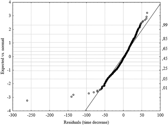
Normality of residuals of time decrease in final GLM model (solid line sets out the course of normal distribution).

Fig. A2.

Scatterplots for explanatory variables (predictors).

References

- Economist . 2020. Many Britons Are Not Taking Social Distancing for COVID-19 Seriously. (Econ) [Google Scholar]
- Agüero F., Adell M.N., Pérez Giménez A., López Medina M.J., Garcia Continente X. Adoption of preventive measures during and after the 2009 influenza A (H1N1) virus pandemic peak in Spain. Prev. Med. (Baltim). 2011;53:203–206. doi: 10.1016/j.ypmed.2011.06.018. [DOI] [PMC free article] [PubMed] [Google Scholar]
- Aguiléra A., Grébert J. Passenger transport mode share in cities: exploration of actual and future trends with a worldwide survey. Int. J. Automot. Technol. Manag. 2014;14:203. doi: 10.1504/IJATM.2014.065290. [DOI] [Google Scholar]
- Anzai A., Kobayashi T., Linton N.M., Kinoshita R., Hayashi K., Suzuki A., Yang Y., Jung S., Miyama T., Akhmetzhanov A.R., Nishiura H. Assessing the impact of reduced travel on exportation dynamics of novel coronavirus infection (COVID-19) J. Clin. Med. 2020;9:601. doi: 10.3390/jcm9020601. [DOI] [PMC free article] [PubMed] [Google Scholar]
- Atchison C.J., Bowman L., Vrinten C., Redd R., Pristera P., Eaton J.W., Ward H. Perceptions and behavioural responses of the general public during the COVID-19 pandemic: a cross-sectional survey of UK adults. medRxiv. 2020 doi: 10.1101/2020.04.01.20050039. [DOI] [PMC free article] [PubMed] [Google Scholar]
- Bajardi P., Poletto C., Ramasco J.J., Tizzoni M., Colizza V., Vespignani A. Human mobility networks, travel restrictions, and the global spread of 2009 H1N1 pandemic. PLoS One. 2011;6 doi: 10.1371/journal.pone.0016591. [DOI] [PMC free article] [PubMed] [Google Scholar]
- Belik V.V., Geisel T., Brockmann D. 2009 International Conference on Computational Science and Engineering. IEEE. 2009. The Impact of Human Mobility on Spatial Disease Dynamics; pp. 932–935. [DOI] [Google Scholar]
- Biscayart C., Angeleri P., Lloveras S., Chaves, T. do S.S., Schlagenhauf, P., Rodríguez-Morales, A.J The next big threat to global health? 2019 novel coronavirus (2019-nCoV): what advice can we give to travellers? – interim recommendations January 2020, from the Latin-American society for Travel Medicine (SLAMVI) Travel Med. Infect. Dis. 2020;33:17–20. doi: 10.1016/j.tmaid.2020.101567. [DOI] [PMC free article] [PubMed] [Google Scholar]
- Bounie D., Camara Y., Galbraith J.W. 2020. Consumers’ Mobility, Expenditure and Online-Offline Substitution Response to COVID-19: Evidence from French Transaction Data. [DOI] [PMC free article] [PubMed] [Google Scholar]
- Buehler R. Determinants of transport mode choice: a comparison of Germany and the USA. J. Transp. Geogr. 2011 doi: 10.1016/j.jtrangeo.2010.07.005. [DOI] [Google Scholar]
- Buliung R.N., Kanaroglou P.S. Urban form and household activity-travel behavior. Growth Chang. 2006 doi: 10.1111/j.1468-2257.2006.00314.x. [DOI] [Google Scholar]
- Camitz M., Liljeros F. The effect of travel restrictions on the spread of a moderately contagious disease. BMC Med. 2006;4:32. doi: 10.1186/1741-7015-4-32. [DOI] [PMC free article] [PubMed] [Google Scholar]
- Casas I., Horner M.W., Weber J. A comparison of three methods for identifying transport-based exclusion: a case study of children’s access to urban opportunities in Erie and Niagara Counties, New York. Int. J. Sustain. Transp. 2009 doi: 10.1080/15568310802158761. [DOI] [Google Scholar]
- Chan H.F., Skali A., Savage D., Stadelmann D., Torgler B. 2020. Risk Attitudes and Human Mobility during the COVID-19 Pandemic. CREMA Work. Pap. Ser. [DOI] [PMC free article] [PubMed] [Google Scholar]
- Chen F., Jiang M., Rabidoux S., Robinson S. Public avoidance and epidemics: insights from an economic model. J. Theor. Biol. 2011;278:107–119. doi: 10.1016/j.jtbi.2011.03.007. [DOI] [PubMed] [Google Scholar]
- Chong K.C., Ying Zee B.C. Modeling the impact of air, sea, and land travel restrictions supplemented by other interventions on the emergence of a new influenza pandemic virus. BMC Infect. Dis. 2012;12:309. doi: 10.1186/1471-2334-12-309. [DOI] [PMC free article] [PubMed] [Google Scholar]
- Cooley P., Brown S., Cajka J., Chasteen B., Ganapathi L., Grefenstette J., Hollingsworth C.R., Lee B.Y., Levine B., Wheaton W.D., Wagener D.K. The role of Subway travel in an influenza epidemic: a New York City simulation. J. Urban Heal. 2011;88:982–995. doi: 10.1007/s11524-011-9603-4. [DOI] [PMC free article] [PubMed] [Google Scholar]
- Costa P.B., Neto G.C.M., Bertolde A.I. Urban mobility indexes: abrief review of the literature. Transp. Res. Procedia. 2017;25:3649–3659. doi: 10.1016/j.trpro.2017.05.330. [DOI] [Google Scholar]
- Curtis C., Ellder E., Scheurer J. Public transport accessibility tools matter: a case study of Gothenburg, Sweden. Case Stud. Transp. Policy. 2019 doi: 10.1016/j.cstp.2018.12.003. [DOI] [Google Scholar]
- De Luca G., Van Kerckhove K., Coletti P., Poletto C., Bossuyt N., Hens N., Colizza V. The impact of regular school closure on seasonal influenza epidemics: a data-driven spatial transmission model for Belgium. BMC Infect. Dis. 2018;18:29. doi: 10.1186/s12879-017-2934-3. [DOI] [PMC free article] [PubMed] [Google Scholar]
- Delaney L., Kleczkowski A., Maharaj S., Rasmussen S., Williams L. Reflections on a virtual experiment addressing human behavior during epidemics. Simul. Ser. 2013;45:131–138. [Google Scholar]
- Delisle Nyström C., Barnes J.D., Blanchette S., Faulkner G., Leduc G., Riazi N.A., Tremblay M.S., Trudeau F., Larouche R. Relationships between area-level socioeconomic status and urbanization with active transportation, independent mobility, outdoor time, and physical activity among Canadian children. BMC Public Health. 2019;19:1–13. doi: 10.1186/s12889-019-7420-y. [DOI] [PMC free article] [PubMed] [Google Scholar]
- Ebrahim S.H., Ahmed Q.A., Gozzer E., Schlagenhauf P., Memish Z.A. Covid-19 and community mitigation strategies in a pandemic. BMJ. 2020;368:1–2. doi: 10.1136/bmj.m1066. [DOI] [PubMed] [Google Scholar]
- Engle S., Stromme J., Zhou A. 2020. Staying at Home: Mobility Effects of COVID-19*. [Google Scholar]
- Engle S., Stromme J., Zhou A. 2020. Staying at Home: Mobility Effects of COVID-19 *. [Google Scholar]
- Epstein J.M., Goedecke D.M., Yu F., Morris R.J., Wagener D.K., Bobashev G.V. Controlling pandemic flu: the value of international air travel restrictions. PLoS One. 2007;2 doi: 10.1371/journal.pone.0000401. [DOI] [PMC free article] [PubMed] [Google Scholar]
- Fujikoshi Y. Two-way ANOVA models with unbalanced data. Discret. Math. 1993;116:315–334. doi: 10.1016/0012-365X(93)90410-U. [DOI] [Google Scholar]
- Gao S., Rao J., Kang Y., Liang Y., Kruse J. 2020. Mapping County-Level Mobility Pattern Changes in the United States in Response to COVID-19. [Google Scholar]
- Germann T.C., Kadau K., Longini I.M., Macken C.A. Mitigation strategies for pandemic influenza in the United States. Proc. Natl. Acad. Sci. U. S. A. 2006;103:5935–5940. doi: 10.1073/pnas.0601266103. [DOI] [PMC free article] [PubMed] [Google Scholar]
- Giesel F., Nobis C. The impact of Carsharing on Car ownership in German cities. Transp. Res. Procedia. 2016;19:215–224. doi: 10.1016/j.trpro.2016.12.082. [DOI] [Google Scholar]
- Goodwin R., Sun S. Early responses to H7N9 in southern Mainland China. BMC Infect. Dis. 2014;14:1–7. doi: 10.1186/1471-2334-14-8. [DOI] [PMC free article] [PubMed] [Google Scholar]
- Hopkins D. Can environmental awareness explain declining preference for car-based mobility amongst generation Y? A qualitative examination of learn to drive behaviours. Transp. Res. Part A Policy Pract. 2016;94:149–163. doi: 10.1016/j.tra.2016.08.028. [DOI] [Google Scholar]
- Kamruzzaman M., Hine J. Participation index: a measure to identify rural transport disadvantage? J. Transp. Geogr. 2011;19:882–899. doi: 10.1016/j.jtrangeo.2010.11.004. [DOI] [Google Scholar]
- Kim S.J., Han J.A., Lee T.Y., Hwang T.Y., Kwon K.S., Park K.S., Lee K.J., Kim M.S., Lee S.Y. Community-based risk communication survey: risk prevention behaviors in communities during the H1N1 crisis, 2010. Osong Public Heal. Res. Perspect. 2014;5:9–19. doi: 10.1016/j.phrp.2013.12.001. [DOI] [PMC free article] [PubMed] [Google Scholar]
- Klein, B., Larock, T., Mccabe, S., Torres, L., Privitera, F., Lake, B., Kraemer, M.U.G., Brownstein, J.S., Lazer, D., Eliassi-Rad, T., Scarpino, S. V, Chinazzi, M., Vespignani, A., 2020. Assessing Changes in Commuting and Individual Mobility in Major Metropolitan Areas in the United States during the COVID-19 Outbreak.
- Ko J., Lee S., Byun M. Exploring factors associated with commute mode choice: an application of city-level general social survey data. Transp. Policy. 2019;75:36–46. doi: 10.1016/j.tranpol.2018.12.007. [DOI] [Google Scholar]
- La Paix Puello L., Chowdhury S., Geurs K. Using panel data for modelling duration dynamics of outdoor leisure activities. J. Choice Model. 2019 doi: 10.1016/j.jocm.2018.03.003. [DOI] [Google Scholar]
- Lavrakas P. 2008. Encyclopedia of Survey Research Methods. [DOI] [Google Scholar]
- Liao Q., Cowling B.J., Wu P., Leung G.M., Fielding R., Lam W.W.T. Population behavior patterns in response to the risk of influenza a(H7N9) in Hong Kong, December 2013–February 2014. Int. J. Behav. Med. 2015;22:672–682. doi: 10.1007/s12529-015-9465-3. [DOI] [PMC free article] [PubMed] [Google Scholar]
- Liu W., Yue X.-G., Tchounwou P.B. Response to the COVID-19 epidemic: the Chinese experience and implications for other countries. Int. J. Environ. Res. Public Health. 2020;17:2304. doi: 10.3390/ijerph17072304. [DOI] [PMC free article] [PubMed] [Google Scholar]
- Lugnér A.K., Postma M.J. Mitigation of pandemic influenza: review of cost–effectiveness studies. Expert Rev. Pharmacoecon. Outcomes Res. 2009;9:547–558. doi: 10.1586/erp.09.56. [DOI] [PubMed] [Google Scholar]
- Ma X., Liu C., Wen H., Wang Y., Wu Y.J. Understanding commuting patterns using transit smart card data. J. Transp. Geogr. 2017;58:135–145. doi: 10.1016/j.jtrangeo.2016.12.001. [DOI] [Google Scholar]
- McDonald N.C. Are millennials really the “go-nowhere” generation? J. Am. Plan. Assoc. 2015;81:90–103. doi: 10.1080/01944363.2015.1057196. [DOI] [Google Scholar]
- Meier K., Glatz T., Guijt M.C., Piccininni M., Van Der Meulen M., Atmar K., Jolink A.C., Kurth T., Rohmann J.L., Najafabadi A.H.Z., Andour L., Blommaart L., Fisher F.L., Splinter B., Teunissen M., Rohmann G. 2020. Public Perspectives on Social Distancing and Other Protective Measures in Europe: ACross-Sectional Survey Study during the COVID-19 Pandemic. [DOI] [PMC free article] [PubMed] [Google Scholar]
- Mirsoleymani S., Nekooghadam S. Mojtaba. Risk factors for severe coronavirus disease 2019 (COVID-19) among Iranian patients: who was more vulnerable? SSRN Electron. J. 2020 doi: 10.2139/ssrn.3566216. [DOI] [Google Scholar]
- Musselwhite C., Avineri E., Susilo Y. Editorial JTH 16 –The Coronavirus Disease COVID-19 and implications for transport and health. J. Transp. Heal. 2020 doi: 10.1016/j.jth.2020.100853. [DOI] [PMC free article] [PubMed] [Google Scholar]
- Olawole M.O., Aloba O. Mobility characteristics of the elderly and their associated level of satisfaction with transport services in Osogbo, Southwestern Nigeria. Transp. Policy. 2014;35:105–116. doi: 10.1016/j.tranpol.2014.05.018. [DOI] [Google Scholar]
- Paddeu D., Parkhurst G., Fancello G., Fadda P., Ricci M. Multi-stakeholder collaboration in urban freight consolidation schemes: drivers and barriers to implementation. Transport. 2018;33:913–929. doi: 10.3846/transport.2018.6593. [DOI] [Google Scholar]
- Pasaoglu G., Zubaryeva A., Fiorello D., Thiel C. Analysis of European mobility surveys and their potential to support studies on the impact of electric vehicles on energy and infrastructure needs in Europe. Technol. Forecast. Soc. Change. 2014 doi: 10.1016/j.techfore.2013.09.002. [DOI] [Google Scholar]
- de Paz C., Muller M., Munoz Boudet A.M., Gaddis I. 2020. Gender Dimensions of the COVID-19 Pandemic. [Google Scholar]
- Permana A.S., Muhamad Ludin A.N., Perera R. Prediction of Citizens’ Decisions on Transport Mode Choice in Bandung City, Indonesia by Using General Linear Model Given existing Level of Pedestrian Friendly Environment. Int. J. Sci. Eng. 2014;6:102–111. doi: 10.12777/ijse.6.2.102-111. [DOI] [Google Scholar]
- Poletti P., Ajelli M., Merler S. Risk perception and effectiveness of uncoordinated behavioral responses in an emerging epidemic. Math. Biosci. 2012;238:80–89. doi: 10.1016/J.MBS.2012.04.003. [DOI] [PubMed] [Google Scholar]
- Poletto C., Gomes M.F., Pastore Piontti A., Rossi L., Bioglio L., Chao D.L., Longini I.M., Halloran M.E., Colizza V., Vespignani A. Assessing the impact of travel restrictions on international spread of the 2014 West African Ebola epidemic. Euro Surveill. 2014:19. doi: 10.2807/1560-7917.es2014.19.42.20936. [DOI] [PMC free article] [PubMed] [Google Scholar]
- Poletto C., Tizzoni M., Colizza V. Human mobility and time spent at destination: impact on spatial epidemic spreading. J. Theor. Biol. 2013;338:41–58. doi: 10.1016/J.JTBI.2013.08.032. [DOI] [PubMed] [Google Scholar]
- Pullano G., Valdano E., Scarpa N., Rubrichi S., Colizza V. 2020. Population Mobility Reductions during COVID-19 Epidemic in France under Lockdown. [DOI] [PMC free article] [PubMed] [Google Scholar]
- Rollinson P.A. The spatial isolation of elderly single-room-occupancy hotel tenants. Prof. Geogr. 1991 doi: 10.1111/j.0033-0124.1991.00456.x. [DOI] [Google Scholar]
- Rubin G.J., Amlôt R., Page L., Wessely S. Public perceptions, anxiety, and behaviour change in relation to the swine flu outbreak: cross sectional telephone survey. BMJ. 2009;339:156. doi: 10.1136/bmj.b2651. [DOI] [PMC free article] [PubMed] [Google Scholar]
- Ryan J., Wretstrand A., Schmidt S.M. Exploring public transport as an element of older persons’ mobility: acapability approach perspective. J. Transp. Geogr. 2015;48:105–114. doi: 10.1016/j.jtrangeo.2015.08.016. [DOI] [Google Scholar]
- Sadique M.Z., Edmunds W.J., Smith R.D., Meerding W.J., de Zwart O., Brug J., Beutels P. Precautionary behavior in response to perceived threat of pandemic influenza. Emerg. Infect. Dis. 2007;13:1307–1313. doi: 10.3201/eid1309.070372. [DOI] [PMC free article] [PubMed] [Google Scholar]
- Schönfelder S., Axhausen K.W. Activity spaces: measures of social exclusion? Transp. Policy. 2003 doi: 10.1016/j.tranpol.2003.07.002. [DOI] [Google Scholar]
- Schwanen T., Dieleman F.M., Dijst M. Travel behaviour in Dutch monocentric and policentric urban systems. J. Transp. Geogr. 2001 doi: 10.1016/S0966-6923(01)00009-6. [DOI] [Google Scholar]
- Siren A., Haustein S. Baby boomers’ mobility patterns and preferences: what are the implications for future transport? Transp. Policy. 2013;29:136–144. doi: 10.1016/j.tranpol.2013.05.001. [DOI] [Google Scholar]
- Sypsa V., Livanios T., Psichogiou M., Hospital L., Malliori M. 2014. P ublic. [Google Scholar]
- Tilley S., Houston D. The gender turnaround: young women now travelling more than young men. J. Transp. Geogr. 2016;54:349–358. doi: 10.1016/j.jtrangeo.2016.06.022. [DOI] [Google Scholar]
- Turcotte M. Life in metropolitan areas. The city/suburb contrast: how can we measure it? Can. Soc. Trends. Stat. Canada - Cat. 2006:2–19. [Google Scholar]
- Van Herck K., Castelli F., Zuckerman J., Nothdurft H., Van Damme P., Dahlgren A.-L., Gargalianos P., Lopéz-Vélez R., Overbosch D., Caumes E., Walker E., Gisler S., Steffen R. Knowledge Attitudes and Practices in Travel-related Infectious Diseases: The European Airport Survey. J. Travel Med. 2004;11:3–8. doi: 10.2310/7060.2004.13609. [DOI] [PubMed] [Google Scholar]
- de Vos J. The effect of COVID-19 and subsequent social distancing on travel behavior. Transp. Res. Interdiscip. Perspect. 2020;5 doi: 10.1016/j.trip.2020.100121. [DOI] [PMC free article] [PubMed] [Google Scholar]
- Wu Y., Pu C., Li L., Zhang G. Traffic-driven epidemic spreading and its control strategies. Digit. Commun. Networks. 2019;5:56–61. doi: 10.1016/J.DCAN.2018.10.005. [DOI] [Google Scholar]
- Yang X.-H., Wang B., Chen S.-Y., Wang W.-L. Epidemic dynamics behavior in some bus transport networks. Phys. A Stat. Mech. its Appl. 2012;391:917–924. doi: 10.1016/J.PHYSA.2011.08.070. [DOI] [Google Scholar]
- Yap J., Lee V.J., Yau T.Y., Ng T.P., Tor P.C. Knowledge, attitudes and practices towards pandemic influenza among cases, close contacts, and healthcare workers in tropical Singapore: a cross-sectional survey. BMC Public Health. 2010;10 doi: 10.1186/1471-2458-10-442. [DOI] [PMC free article] [PubMed] [Google Scholar]
- Yilmazkuday H. 2020. International Evidence from Google Mobility Data. [Google Scholar]
- Zhao S., Wu C.H., Kuang Y., Ben-Arieh D. Information dissemination and human behaviors in epidemics. IIE Annu. Conf. Expo. 2015;2015:1907–1915. [Google Scholar]