Rapid prediction of protein natural frequencies using graph neural networks

Abstract

Natural vibrational frequencies of proteins help to correlate functional shifts with sequence or geometric variations that lead to negligible changes in protein structures, such as point mutations related to disease lethality or medication effectiveness. Normal mode analysis is a well-known approach to accurately obtain protein natural frequencies. However, it is not feasible when high-resolution protein structures are not available or time consuming to obtain. Here we provide a machine learning model to directly predict protein frequencies from primary amino acid sequences and low-resolution structural features such as contact or distance maps. We utilize a graph neural network called principal neighborhood aggregation, trained with the structural graphs and normal mode frequencies of more than 34 000 proteins from the protein data bank. combining with existing contact/distance map prediction tools, this approach enables an end-to-end prediction of the frequency spectrum of a protein given its primary sequence.

We present a computational framework based on graph neural networks (GNNs) to predict the natural frequencies of proteins from primary amino acid sequences and contact/distance maps.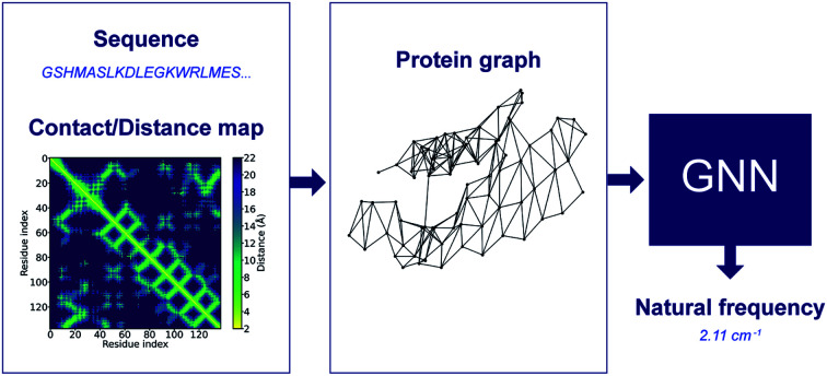

Introduction

Enormous efforts have been devoted to investigate the structure and functionality of proteins, the building blocks of life.^1–3 An important feature of proteins is their continuous motion or vibration.⁴ Even sequence or geometric variations that lead to negligible structural changes can affect the low-frequency motions of proteins,^5,6 and in turn, the vibrational modes can be utilized to identify key mutations associated to drug design,⁷ diseases,^8–10 or many other biophysical phenomena in living organisms, and in biomaterials more broadly.¹¹ As the imaging resolution provided by the state-of-the-art technology is still insufficient to measure the lowest natural frequency of most protein structures, a computational approach called normal mode analysis (NMA) is generally adopted to calculate the vibrational modes if the high-resolution atomistic structures of proteins and force fields that define interatomic interactions are available.^4,12

Nevertheless, NMA calculation is quite time and memory consuming, especially for large protein structures, and machine learning (ML) techniques can help to enable fast prediction of protein natural frequencies.¹² Recent development in ML has driven great success in computer vision, natural language processing and autonomous driving.¹³ Breakthroughs continue to be made in molecular and materials science,^14–18 biology and medicine,^19,20 including design of composites and bio-inspired materials,^21–28 as well as protein design and sonification.^29–34 To predict the natural frequencies of protein molecules, in earlier work a data-driven model was proposed, based on a feedforward neural network and trained the model with five structural features of protein molecules, including the largest and smallest diameters as well as the contents of α-helix, β-strand and 3–10 helix domains.¹² These features can be collected from experiments or computations, but it is challenging to obtain them from protein primary sequences only. Therefore, this model has difficulties in identifying the direct relationship between the primary sequences and natural frequencies of proteins.

To overcome this limitation and thus enable an end-to-end prediction of protein frequency spectrum, i.e., from primary sequence to natural frequencies, we developed a computational framework based on graph neural networks (GNNs). Unlike standard neural networks that operate on Euclidean data (e.g., pixels in images and words in text), GNNs, as the name implies, operate on graphs that consist nodes connected by edges without natural orders, and hence form non-Euclidean data structures.³⁵ GNN models have been employed in materials research tasks such as hardness prediction,³⁶ and architected materials design,³⁷ and they have demonstrated outstanding performance on learning molecular structures,^38–40 and designing proteins.^41,42 In this work, a GNN model is developed to predict protein frequencies from primary sequences and low-resolution structural features such as contact or distance maps. The integration of this model with one of existing contact/distance map prediction tools^43–45 gives, to the best of our knowledge, the first end-to-end approach to predict the natural frequencies of a protein given its primary sequence.

Results and discussion

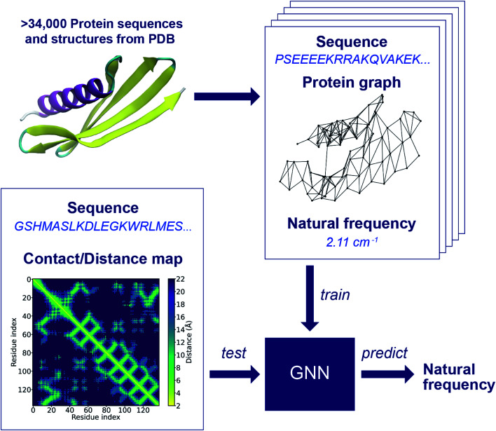
The workflow of the approach for protein frequency prediction using GNNs is schematically shown in Fig. 1. The inputs to the GNN are graphs that represent proteins. In a supervised learning task of frequency prediction, graphs in the training set (denoted henceforth as training graphs) are labeled with natural frequencies and are fed into the GNN for training. Then, the trained GNN takes as input unlabeled graphs of test proteins (denoted as test graphs) and outputs the prediction of the labels, i.e., the natural frequencies of these proteins. Each training graph consists of the following components: connectivity, node feature, edge feature, and label. The connectivity stands for a data structure that tells whether two nodes are connected or not. In a protein graph, each node represents an amino acid residue with its amino acid code defined as the node feature. Two nodes are connected by an edge if the distance between the Cα atoms of the residues that those two nodes represent is less than a threshold value. According to the way we define edges in protein graphs, the adjacency matrix of a graph is in fact the contact map of the corresponding protein (see Fig. S1 in ESI†). If the distance map (or distance matrix) of a protein is known, we can denote the Cα–Cα distance between a pair of residues as the feature of the corresponding edge. To label the protein graphs, we leverage a database of the first 64 normal modes of more than 100 000 protein structures from PDB.⁴ Each graph is labeled with a natural frequency corresponding to one of the 64 normal modes. During the conversion of protein structure into graphs, protein graphs that contains different numbers of nodes in PDB and Dictionary of Protein Secondary Structure (DSSP),⁴⁶ isolated nodes, or outliers in the frequency distribution of the database are excluded to simplify data preprocessing and to improve training speed and prediction accuracy. As a result, more than 42 000 protein graphs are generated, and they are randomly split into a training set of ∼34 000 graphs, a validation set of ∼4000 graphs and a test set of ∼4000 graphs. There may exist structural similarities among training, validation and test sets due to the random split, while its effect on the model performance will be left to a future study. Fig. S2† shows a comparison between the frequency distributions in the raw database and in the preprocessed protein graphs. The preprocessing here could benefit the model performance as the preprocessed dataset is less skewed than the raw database, and proteins with extremely low 1st and 2nd natural frequencies are excluded. Yet, a bias may still exist in the preprocessed dataset. The impact of the skewed distributions can potentially be reduced by techniques such as stratification, which will be implemented in a future study. New test graphs can be constructed from sequences and distance or contact maps following the same way.

Fig. 1. Schematic of the training and test processes of the graph neural network (GNN) for protein frequency prediction. Protein sequences and structures from the Protein Data Bank (PDB) are represented as graphs in which each node denotes a residue with its amino acid code defined as the feature of the node, and two residues are connected by an edge if the distance between their Cα atoms is less than a threshold value. Each protein graph is labeled with a natural frequency corresponding to a normal mode calculated from the normal mode analysis (NMA). Labeled protein graphs forms the training set of the GNN model, as ground truth. The GNN is trained to learn a graph embedding that correlates protein graphs with natural frequencies. The trained model is able to predict the natural frequency of a protein of which a test graph can be constructed by the sequence and contact/distance map using the same graph representation as in the generation of training graphs.

The GNN is trained with the training set to learn how to translate protein graphs into a graph embedding that can be used to predict protein frequencies. The GNN not only aggregates the node and edge features through the connectivity of the input graph, but also parses simple features into abstract features. It might be difficult to explicitly interpret the physical meanings of these abstract features. However, they form a graph embedding that can represent implicit properties of proteins, and the function of this graph embedding is similar to that of the structural features, for example, the diameter of the protein structure, adopted in a previous work.¹² One of the differences between the current approach and the previous work lies in the extraction of the global features: the graph embedding is learned from simple features using GNNs with deep learning techniques, rather than manually selected. In this regard, the performance of the feedforward neural network adopted in the previous work and the GNN cannot be directly compared since these two networks require different data structures as input. To predict the frequencies of a test protein, structural features such as the largest and smallest diameters, the contents of α-helix, β-strand and 3–10 helix domains should be obtained for the feedforward neural network in the previous work, while the sequence and contact/distance map of the test protein are needed for the GNN. The advantage of this input data structure for the GNN is that there are existing contact/distance map prediction tools, and we rely only on the GNN to bridge the gap between the local structural information and the global features that relate to natural frequencies, which is one of the key tasks in our end-to-end approach for protein frequency prediction. Frequency prediction is a graph regression task that poses particular challenges, and for which earlier GNN architectures do not work well. In this work, we adopt a GNN with a principal neighborhood aggregation graph convolution operator (PNAConv),⁴⁷ which has outperformed many popular GNN models in the literature, such as GCN,⁴⁸ GAT,⁴⁹ GIN,⁵⁰ and MPNN,³⁹ on benchmark tasks for graph regression. The improvement of the performance of the GNN is attributed to the strategies of combining multiple aggregators with degree-based scalers that amplify or attenuate signals in the network according to node degree.

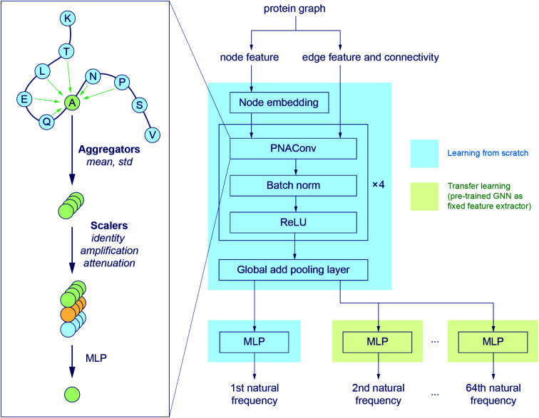
Fig. 2 illustrates the architecture of the GNN, where the node feature of the input graph is firstly translated via a node embedding layer, and then fed into a PNAConv layer along with the edge feature and connectivity of the graph. The PNAConv layer outputs the hidden features of the nodes in the graph by aggregating the information from the neighbors of each node. A sequential block comprised of a PNAConv layer, a batch normalization layer and a Rectified Linear Unit (ReLU) activation function is repeated 4 times to successively generate new representations (or embeddings) for each node. A global pooling layer outputs a graph-level embedding by adding node embeddings across the node, and it is connected to a multilayer perceptron (MLP) that returns a predicted natural frequency. The entire GNN is trained from scratch using the training graphs labeled with the first natural frequency. Here we leverage a transfer learning approach called feature extraction to accelerate the training of the networks for the prediction of the frequencies that correspond to other modes. The pre-trained GNN except the last MLP, for the prediction of the first natural frequency, serves as a feature extractor with the weights for the network fixed. The last MLP is then replaced with a new one with random weights, and only this new MLP is trained with the training graphs labeled with the second or higher natural frequency. The model for the first natural frequency prediction was chosen to be trained from scratch instead of other models because we aim to obtain a slightly higher accuracy for the first natural frequency than others as it corresponds to the normal mode with the lowest non-trivial frequency. In addition, better performance might be achieved by slowly unfreezing pre-trained GNN layers during transfer learning, which will be left to a future study. More details about the layers in the model and the training procedure are given in the Methods section.

Fig. 2. GNN architecture. The node embedding, edge features and connectivity of protein graphs are input to a graph convolution operator named PNAConv where the information from the neighbors of each node in the graph is aggregated to update the hidden features of the node.⁴⁷ The GNN is trained from scratch to predict the first natural frequency. A transfer learning technique is implemented to accelerate the training of the networks for the prediction of other normal mode frequencies.

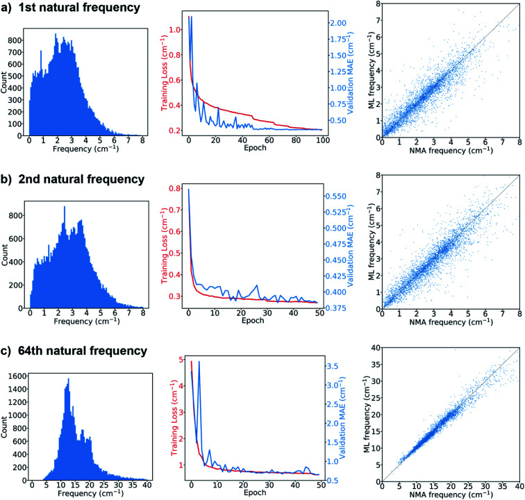
The results from the models for the prediction of the 1st, 2nd or 64th natural frequency are shown in Fig. 3. The mean and standard deviation of the frequency distribution in the training set for the 64th frequency are obviously higher than those for the first two natural frequencies. The learning curves show the evolution of the training loss, which is the mean absolute errors (MAEs) between the ML-predicted frequencies (denoted as ML frequencies) and NMA-calculated frequencies (denoted as NMA frequencies) over the training set, as well as the evolution of the MAEs over the validation set (denoted as validation MAE). The model's hyperparameters were tuned to minimize the validation MAE. For the 1st natural frequency prediction, the final validation MAE is 0.357 cm⁻¹ after tuning, less than 1.36 cm⁻¹, the standard deviation of the frequencies in the validation set. For the 2nd natural frequency, the final validation MAE of the model trained via transfer learning is 0.383 cm⁻¹, slightly greater than 0.356 cm⁻¹, the final validation MAE of the same model trained from scratch (see the comparison in Fig. S3†), but still less than 1.49 cm⁻¹, the standard deviation in the validation set. For the 64th natural frequency, the final validation MAE elevates from 0.44 cm⁻¹ for learning from scratch to 0.66 cm⁻¹ for transfer learning, but it is much less than 5.75 cm⁻¹, the standard deviation in the validation set. Therefore, training via transfer learning does not sacrifice too much accuracy, and this technique offers great benefits as it accelerates the training process by ∼70% per epoch and consumes less GPU memory compared to training from scratch. The feasibility of transfer learning demonstrates that the feature extractor has successfully learned how to translate a protein graph into a graph-level embedding vector that can be used to predict natural frequencies corresponding to different normal modes. After the GNN model is trained, it takes only about 30 seconds to predict the natural frequencies of ∼4000 proteins in the test set that has at least low-resolution structural features such as contact/distance map. The GNN-based approach is much faster than NMA, which takes about 80 min to calculate the frequency spectrum of a single protein structure with ∼120 amino acids. The comparison between the ML and NMA frequencies over the test set is also shown in Fig. 3. Each point represents a test protein with its ML and NMA frequencies denoted as the vertical and horizontal coordinates of the point, respectively. Most of the points are close to the diagonal line, especially in the prediction of the 64th natural frequency, consistent with the comparison between the final validation MAEs and standard deviations in the validation sets since the predictions of the models over the validation and test sets give similar MAEs. A possible mechanism to explain the higher accuracy in the prediction of high-order natural frequencies is that the vibrations of high-order normal modes are more localized in protein structures than those of low-order normal modes, and thus are easier to be learned by the GNN architecture. Fig. S4† compares the performance of the model on the proteins with different numbers of amino acids in the test set. In comparison with short (<100 amino acids) or long (≥500 amino acids) protein sequences, proteins with intermediate lengths achieve higher accuracy in the natural frequency prediction. The deviation in the accuracy with respect to the sequence length may be attributed to few edges in the graphs of the proteins with short sequences as well as a small fraction of very long protein sequences in the training set. In summary, the model prediction agrees very well with the ground truth if the graphs obtained from accurate protein distance (or contact) maps are fed as input.

Fig. 3. Frequency distribution in the training set (left), learning curve (middle), and comparison between the ML-predicted and NMA-calculated frequencies of proteins in the test set (right) for the (a) 1st, (b) 2nd, (c) 64th natural frequency.

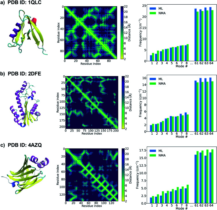
When the accurate contact or distance maps of test proteins are not available, a contact/distance map prediction tool can be leveraged to get the structural features that are needed to construct protein graphs. Here we combine our GNN model with an open-source protein distance prediction network, ProSPr,⁴³ for an end-to-end prediction of the frequency spectrum of a protein given its primary sequence. Fig. 4 shows the 1st–8th and 61–64th frequencies of three proteins (PDB IDs: 1QLC, 2DFE, and 4AZQ) in the test set. The primary sequence of each test protein is fed as input to ProSPr, and the distance map predicted by ProSPr along with the sequence are the features needed to construct a test graph that can be fed into our GNN models to predict the normal mode frequencies. It is shown that the ML frequencies obtained using this end-to-end approach agree well with the corresponding NMA frequencies. This is attributed to the high accuracy of the frequency prediction model using GNN as well as the accurate distance map prediction by ProSPr on these test proteins (Fig. S5†). The ML frequencies may deviate from the NMA frequencies when the distance map predicted by ProSPr is not sufficiently accurate (Fig. S6†), but this issue could be addressed if more accurate protein distance prediction methods are available. We also test our GNN model with the distance maps predicted by AlphaFold 1.⁴⁴ Although it is difficult to test any protein sequence of interest since the feature generation code of AlphaFold 1 is not open-sourced, AlphaFold 1 provides the input features of the CASP13 targets,⁵¹ and thus we can get the distance maps of the CASP13 targets predicted by AlphaFold 1, which are further fed as input to our GNN model. It is worth pointing out that the structures of the CASP 13 targets were published later than the generation of the database of protein natural frequencies that we used to construct the training, validation and test sets in this work. Again, the performance of the protein frequency prediction relies on the accuracy of the distance map prediction (Fig. S7†). The frequencies predicted by the GNN model agree well with the NMA frequencies when AlphaFold 1 predicts a sufficiently accurate distance map (see Fig. S7a†). We note that the ML frequency does not always increase monotonously with the number of the normal mode in Fig. 4. This might be resolved by training a single model that can predict a monotonically increasing frequency spectrum by adding a penalty term in the loss function, and it deserves a study of its own right. Our model is able to provide a good estimation of the frequency corresponding to each normal mode of a test protein from its primary sequence only.

Fig. 4. PDB structure (left), distance map predicted by ProSPr (middle),⁴³ and the 1st–8th and 61–64th frequencies (right) of a test protein with a PDB ID of (a) 1QLC, (b) 2DFE, (c) 4AZQ. The PDB structures of the proteins are shown here for demonstration purposes. Only the primary sequence is input to ProSPr to predict the distance map that is used to construct the test graph. The natural frequencies predicted by the GNN model using these test graphs are compared with the corresponding frequencies calculated from NMA.

Conclusion

We developed a computational framework based on GNNs, trained with more than 34 000 protein graphs, to output the natural frequencies of proteins from primary amino acid sequences and low-resolution structural features such as contact or distance maps. Integration of the GNN model with a protein distance prediction network provides an end-to-end approach to predict protein frequencies given primary sequences. The frequency spectrum predicted by the ML models shows good agreement with that obtained from NMA. Moreover, the standalone GNN model can be utilized as a quick screening tool to identify key point mutations that can significantly affect protein vibrational behaviors, which deserves a study of its own right and will be left to a future study. It has been demonstrated that GNNs are very powerful in learning useful embeddings from graph representation of proteins, and thus would be important tools to predict protein-level properties in graph regression tasks, such as natural frequencies in this work. In addition, GNNs can be utilized to solve node regression tasks in order to predict residue-level properties of proteins. Rapid development in ML techniques is offering exciting pathways to bridge the gaps among protein sequences, structures and properties, and would revolutionize the way we understand and design proteins.

Methods

Data preparation

The atomic coordinates in the proteins are extracted to compute contact/distance maps using the PDB and DSSP modules in Biopython.⁵² Fig. S1† shows the graphs and the corresponding adjacency matrices of an example protein (PDB ID: 4R80) with different threshold distances. It should be pointed out that the atomic coordinates in the proteins are not assigned as node features and are not utilized to train the models. We use the Cartesian coordinates of Cα atoms just to schematically plot the graphs of the example protein. A threshold distance of 12 Å is adopted to define edges in protein graphs used in our computational experiments as it gives low mean absolute error (MAE), as shown in Fig. S8,† and does not exceed the memory limit of the GPU during training. In the database of the normal modes of protein structures, the last 64 normal modes amongst the 70 generated are selected to train the model as the first 6 modes are so-called trivial modes with zero frequency, corresponding to rigid-body translation and rotation. A bash script, including a block normal mode method^53,54 in CHARMM for NMA on each protein structure, was used to automatically download, clean and analyze protein structures. In the database, there are 110 511 protein structures that are composed of standard amino acids only from the Protein Data Bank at the time of database construction.⁴

Graph neural networks (GNNs)

The GNN model is developed based on the deep-learning framework PyTorch⁵⁵ and its geometric extension library PyTorch Geometric.⁵⁶ In the GNN architecture, the node embedding layer has a dictionary size of 20 (i.e., the number of the types of standard amino acids) and outputs each embedding vector with a size of 75. If distance map is known, the edge feature can be represented by the value of the Cα–Cα distance, the reciprocal of the distance, or the distance embedding. For the distance embedding, a distance range of 2–12 Å is equally divided into 10 bins, and the bin number of the distance is input to an edge embedding layer that outputs each embedding vector with a size of 50. If contact map is known but the values of Cα–Cα distances are not available, the edge feature vector is filled by zeros as placeholders, denoted as “no edge feature”. Fig. S9† shows that different representations of edge feature give no significant difference in the final validation MAE. In other words, training with distance maps and training with contact maps have similar performance. The GNN models presented in this paper are trained using the value of the Cα–Cα distance as the edge feature.

The PNAConv layer is a GNN layer where the Principal Neighborhood Aggregation (PNA) operator is embedded within the framework of a message passing neural network:³⁹

1

where X_i^(t) is the feature of the node i at time step t, E_j,i is the feature of the edge (j, i), M and U denote MLPs, 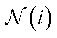is the set of indices of the neighbors of the node i, and ⊕ represents the PNA operator.⁴⁷ In our work, the PNA operator includes 3 scalers (identity, amplification, attenuation) and only 2 aggregators (mean, std) instead of all of the 4 aggregators proposed in original PNA paper⁴⁷ because the removal of the other 2 aggregators (max, min) gives better performance in our preliminary computational experiments (Fig. S10†). The sizes of each input and output sample of the PNAConv layer are equal to 75.

The last MLP that returns the predicted natural frequency has a structure of an input layer of size 75, a hidden layer of size 50, another hidden layer of size 25, and an output layer of one neuron. ReLU is adopted as the activation function in this MLP. We adopt default weight and bias initialization of all of the layers in the model defined by PyTorch Geometric.

Model training and testing

During training, we minimize the MAE between the model output and the target. The models were trained with a batch size of 32 using the Adam optimization method,⁵⁷ for 100 epochs when training from scratch, or for 50 epochs when transfer learning is used to train the last MLP. Early stopping is not used here but it may result in a slightly better performance. Training starts with a learning rate of 0.001, and a dynamic learning rate scheduler named ReduceLROnPlateau reduces the learning rate by half if no improvement is seen for 10 epochs to minimize the validation MAE. We trained and tested the GNN models on a single NVIDIA Quadro RTX 4000 graphic card with 8 GB memory on a local workstation, or on a single NVIDIA Tesla V100 graphic card with 32 GB memory in a cluster.

Data availability

The data file, the code for data pre-processing and model training, and the trained models for testing new proteins in this study are available at GitHub, https://github.com/lamm-mit/ProteinMechanicsGNN and Zenodo for the dataset: DOI: 10.5281/zenodo.6346661.

Conflicts of interest

The authors declare no conflict of interests.

References

- Marcotte E. M. Pellegrini M. Ng H.-L. Rice D. W. Yeates T. O. Eisenberg D. Science. 1999;285:751–753. doi: 10.1126/science.285.5428.751. [DOI] [PubMed] [Google Scholar]
- Berman H. M. Westbrook J. Feng Z. Gilliland G. Bhat T. N. Weissig H. Shindyalov I. N. Bourne P. E. Nucleic Acids Res. 2000;28:235–242. doi: 10.1093/nar/28.1.235. [DOI] [PMC free article] [PubMed] [Google Scholar]
- Cranford S. W. and Buehler M. J., Biomateriomics, Springer, 2012 [Google Scholar]
- Qin Z. Buehler M. J. Extreme Mechanics Letters. 2019;29:100460. doi: 10.1016/j.eml.2019.100460. [DOI] [PMC free article] [PubMed] [Google Scholar]
- Rischel C. Spiedel D. Ridge J. P. Jones M. R. Breton J. Lambry J.-C. Martin J.-L. Vos M. H. Proc. Natl. Acad. Sci. U. S. A. 1998;95:12306–12311. doi: 10.1073/pnas.95.21.12306. [DOI] [PMC free article] [PubMed] [Google Scholar]
- Rodrigues C. H. Pires D. E. Ascher D. B. Nucleic Acids Res. 2018;46:W350–W355. doi: 10.1093/nar/gky300. [DOI] [PMC free article] [PubMed] [Google Scholar]
- Teague S. J. Nat. Rev. Drug Discovery. 2003;27(2):527–541. doi: 10.1038/nrd1129. [DOI] [PubMed] [Google Scholar]
- Xu Z. Paparcone R. Buehler M. J. Biophys. J. 2010;98:2053–2062. doi: 10.1016/j.bpj.2009.12.4317. [DOI] [PMC free article] [PubMed] [Google Scholar]
- Yoon G. Kwak J. Kim J. I. Na S. Eom K. Adv. Funct. Mater. 2011;21:3454–3463. doi: 10.1002/adfm.201002493. [DOI] [Google Scholar]
- Hu Y. Buehler M. J. Matter. 2020;4:265–275. doi: 10.1016/j.matt.2020.10.032. [DOI] [PMC free article] [PubMed] [Google Scholar]
- Kang J. Steward R. L. Kim Y. T. Schwartz R. S. LeDuc P. R. Puskar K. M. J. Theor. Biol. 2011;274:109–119. doi: 10.1016/j.jtbi.2011.01.011. [DOI] [PMC free article] [PubMed] [Google Scholar]
- Qin Z. Yu Q. Buehler M. J. RSC Adv. 2020;10:16607–16615. doi: 10.1039/C9RA04186A. [DOI] [PMC free article] [PubMed] [Google Scholar]
- Lecun Y. Bengio Y. Hinton G. Nature. 2015;521:436–444. doi: 10.1038/nature14539. [DOI] [PubMed] [Google Scholar]
- Liu Y. Zhao T. Ju W. Shi S. Shi S. Shi S. J. Mater. 2017;3:159–177. [Google Scholar]
- Butler K. T. Davies D. W. Cartwright H. Isayev O. Walsh A. Nature. 2018;559:547–555. doi: 10.1038/s41586-018-0337-2. [DOI] [PubMed] [Google Scholar]
- Brown K. A. Brittman S. Maccaferri N. Jariwala D. Celano U. Nano Lett. 2019;20:2–10. doi: 10.1021/acs.nanolett.9b04090. [DOI] [PubMed] [Google Scholar]
- Zhai C. Li T. Shi H. Yeo J. J. Mater. Chem. B. 2020;8:6562–6587. doi: 10.1039/D0TB00896F. [DOI] [PubMed] [Google Scholar]
- Guo K. Yang Z. Yu C.-H. Buehler M. J. Mater. Horiz. 2021;8:1153–1172. doi: 10.1039/D0MH01451F. [DOI] [PubMed] [Google Scholar]
- Ching T. Himmelstein D. S. Beaulieu-Jones B. K. Kalinin A. A. Do B. T. Way G. P. Ferrero E. Agapow P. M. Zietz M. Hoffman M. M. Xie W. Rosen G. L. Lengerich B. J. Israeli J. Lanchantin J. Woloszynek S. Carpenter A. E. Shrikumar A. Xu J. Cofer E. M. Lavender C. A. Turaga S. C. Alexandari A. M. Lu Z. Harris D. J. Decaprio D. Qi Y. Kundaje A. Peng Y. Wiley L. K. Segler M. H. S. Boca S. M. Swamidass S. J. Huang A. Gitter A. Greene C. S. J. R. Soc., Interface. 2018;15:20170387. doi: 10.1098/rsif.2017.0387. [DOI] [PMC free article] [PubMed] [Google Scholar]
- Alber M. Buganza Tepole A. Cannon W. R. De S. Dura-Bernal S. Garikipati K. Karniadakis G. Lytton W. W. Perdikaris P. Petzold L. Kuhl E. npj Digital Medicine. 2019;2:115. doi: 10.1038/s41746-019-0193-y. [DOI] [PMC free article] [PubMed] [Google Scholar]
- Gu G. X. Chen C. T. Buehler M. J. Extreme Mechanics Letters. 2018;18:19–28. doi: 10.1016/j.eml.2017.10.001. [DOI] [Google Scholar]
- Gu G. X. Chen C. T. Richmond D. J. Buehler M. J. Mater. Horiz. 2018;5:939–945. doi: 10.1039/C8MH00653A. [DOI] [Google Scholar]
- Yu C.-H. Qin Z. Buehler M. J. Nano Futures. 2019;3:035001. doi: 10.1088/2399-1984/ab36f0. [DOI] [Google Scholar]
- Yang Z. Yu C.-H. Buehler M. J. Sci. Adv. 2021;7:eabd7416. doi: 10.1126/sciadv.abd7416. [DOI] [PMC free article] [PubMed] [Google Scholar]
- Yang Z. Yu C. H. Guo K. Buehler M. J. J. Mech. Phys. Solids. 2021;154:104506. doi: 10.1016/j.jmps.2021.104506. [DOI] [Google Scholar]
- Hsu Y.-C. Yu C.-H. Buehler M. J. Matter. 2020;3:197–211. doi: 10.1016/j.matt.2020.04.019. [DOI] [Google Scholar]
- Buehler E. L. Su I. Buehler M. J. Extreme Mechanics Letters. 2021;42:101034. doi: 10.1016/j.eml.2020.101034. [DOI] [Google Scholar]
- Ni B. Gao H. MRS Bull. 2021;46:19–25. doi: 10.1557/s43577-020-00006-y. [DOI] [Google Scholar]
- Yu C.-H. Qin Z. Martin-Martinez F. J. Buehler M. J. ACS Nano. 2019;13:7471–7482. doi: 10.1021/acsnano.9b02180. [DOI] [PubMed] [Google Scholar]
- Franjou S. L. Milazzo M. Yu C.-H. Buehler M. J. Expert Rev. Proteomics. 2019;16:875–879. doi: 10.1080/14789450.2019.1697236. [DOI] [PubMed] [Google Scholar]
- Yu C.-H. Buehler M. J. APL Bioeng. 2020;4:016108. doi: 10.1063/1.5133026. [DOI] [PMC free article] [PubMed] [Google Scholar]
- Buehler M. J. Nano Futures. 2020;4:035004. doi: 10.1088/2399-1984/ab9a27. [DOI] [Google Scholar]
- Qin Z. Wu L. Sun H. Huo S. Ma T. Lim E. Chen P. Y. Marelli B. Buehler M. J. Extreme Mechanics Letters. 2020;36:100652. doi: 10.1016/j.eml.2020.100652. [DOI] [Google Scholar]
- Franjou S. L. Milazzo M. Yu C.-H. Buehler M. J. Nano Futures. 2021;5:012501. doi: 10.1088/2399-1984/abcf1b. [DOI] [Google Scholar]
- Zhou J. Cui G. Hu S. Zhang Z. Yang C. Liu Z. Wang L. Li C. Sun M. AI Open. 2020;1:57–81. doi: 10.1016/j.aiopen.2021.01.001. [DOI] [Google Scholar]
- Mazhnik E. Oganov A. R. J. Appl. Phys. 2020;128:075102. doi: 10.1063/5.0012055. [DOI] [Google Scholar]
- Guo K. Buehler M. J. Extreme Mechanics Letters. 2020;41:101029. doi: 10.1016/j.eml.2020.101029. [DOI] [Google Scholar]
- Duvenaud D. K., Maclaurin D., Iparraguirre J., Bombarell R., Hirzel T., Aspuru-Guzik A. and Adams R. P., in Advances in Neural Information Processing Systems, NIPS, 2015, vol. 28 [Google Scholar]
- Gilmer J., Schoenholz S. S., Riley P. F., Vinyals O. and Dahl G. E., in Proceedings of the 34th International Conference on Machine Learning, ICML, 2017, vol. 70, pp. 1263–1272 [Google Scholar]
- Xie T. Grossman J. C. Phys. Rev. Lett. 2018;120:145301. doi: 10.1103/PhysRevLett.120.145301. [DOI] [PubMed] [Google Scholar]
- Ingraham J., Garg V., Barzilay R. and Jaakkola T., in Advances in Neural Information Processing Systems, NeurIPS, 2019, vol. 32 [Google Scholar]
- Strokach A. Becerra D. Corbi-Verge C. Perez-Riba A. Kim P. M. Cell Syst. 2020;11:402–411.e4. doi: 10.1016/j.cels.2020.08.016. [DOI] [PubMed] [Google Scholar]
- Billings W. M. Hedelius B. Millecam T. Wingate D. Della Corte D. bioRxiv. 2019 doi: 10.1101/830273. [DOI] [Google Scholar]
- Senior A. W. Evans R. Jumper J. Kirkpatrick J. Sifre L. Green T. Qin C. Žídek A. Nelson A. W. R. Bridgland A. Penedones H. Petersen S. Simonyan K. Crossan S. Kohli P. Jones D. T. Silver D. Kavukcuoglu K. Hassabis D. Nature. 2020;577:706–710. doi: 10.1038/s41586-019-1923-7. [DOI] [PubMed] [Google Scholar]
- Ding W. Gong H. Adv. Sci. 2020;7:2001314. doi: 10.1002/advs.202001314. [DOI] [PMC free article] [PubMed] [Google Scholar]
- Kabsch W. Sander C. Biopolymers. 1983;22:2577–2637. doi: 10.1002/bip.360221211. [DOI] [PubMed] [Google Scholar]
- Corso G., Cavalleri L., Beaini D., Liò P. and Veličković P., in Advances in Neural Information Processing Systems, NeurIPS, 2020, vol. 33, pp. 13260–13271 [Google Scholar]
- Kipf T. N. and Welling M., in 5th International Conference on Learning Representations, ICLR, 2017 [Google Scholar]
- Veličković P., Casanova A., Liò P., Cucurull G., Romero A. and Bengio Y., in 6th International Conference on Learning Representations, ICLR, 2017 [Google Scholar]
- Xu K., Hu W., Leskovec J. and Jegelka S., in 7th International Conference on Learning Representations, ICLR, 2018 [Google Scholar]
- Kryshtafovych A. Schwede T. Topf M. Fidelis K. Moult J. Proteins. 2019;87:1011–1020. doi: 10.1002/prot.25823. [DOI] [PMC free article] [PubMed] [Google Scholar]
- Cock P. J. A. Antao T. Chang J. T. Chapman B. A. Cox C. J. Dalke A. Friedberg I. Hamelryck T. Kauff F. Wilczynski B. De Hoon M. J. L. Bioinformatics. 2009;25:1422–1423. doi: 10.1093/bioinformatics/btp163. [DOI] [PMC free article] [PubMed] [Google Scholar]
- Tama F. Gadea F. X. Marques O. Sanejouand Y.-H. Proteins. 2000;41:1–7. doi: 10.1002/1097-0134(20001001)41:1<1::AID-PROT10>3.0.CO;2-P. [DOI] [PubMed] [Google Scholar]
- Ruiz L. Xia W. Meng Z. Keten S. Carbon. 2015;82:103–115. doi: 10.1016/j.carbon.2014.10.040. [DOI] [Google Scholar]
- Paszke A., Gross S., Massa F., Lerer A., Bradbury Google J., Chanan G., Killeen T., Lin Z., Gimelshein N., Antiga L., Desmaison A., Xamla A. K., Yang E., Devito Z., Raison Nabla M., Tejani A., Chilamkurthy S., Ai Q., Steiner B., Facebook L. F., Facebook J. B. and Chintala S., in Advances in Neural Information Processing Systems 32, NIPS, 2019 [Google Scholar]
- Fey M. and Lenssen J. E., in ICLR Workshop on Representation Learning on Graphs and Manifolds, 2019 [Google Scholar]
- Kingma D. P. and Ba J. L., in 3rd International Conference on Learning Representations, ICLR, 2015 [Google Scholar]
Associated Data
This section collects any data citations, data availability statements, or supplementary materials included in this article.
Supplementary Materials
Data Availability Statement