

Abstract
Connectomes derived from resting-state functional MRI scans have significantly benefited from the development of dedicated fMRI motion correction and denoising algorithms. But they are based on empirical correlations that can produce unreliable results in high dimension low sample size settings. A family of statistical estimators, the covariance shrinkage methods, could mitigate this issue. Unfortunately, these methods have rarely been used to correct functional connectomes and no extensive experiment has been conducted so far to compare the shrinkage methods available for this task. In this work, we propose to fix this issue by processing a benchmark dataset made of a thousand high-resolution resting-state fMRI scans provided by the Human Connectome Project to compare the ability of five prominent covariance shrinkage methods to produce reliable functional connectomes at different spatial resolutions and scans duration: the pioneer linear covariance shrinkage method introduced by Ledoit and Wolf, the Oracle Approximating Shrinkage, the QuEST method, the NERCOME method, and a recent analytical approximation of the QuEST approach. Our experiments establish that all covariance shrinkage methods significantly improve functional connectomes derived from short fMRI scans. The Oracle Approximating Shrinkage and the QuEST method produced the best results. Lastly, we present shrinkage intensity charts that can be used for designing and analyzing fMRI studies. These charts indicate that sparse connectomes are difficult to estimate from short fMRI scans, and they describe a range of settings where dynamic functional connectivity should not be computed.
Keywords: Resting-state fmri, Covariance shrinkage, Dynamic connectivity
1. Introduction
Resting-state functional MRI (rs-fMRI) offers a precious insight into brain function by measuring at the scale of the entire brain a Blood-Oxygen-Level-Dependent (BOLD) signal reflecting brain activity over long periods of rest (Fox and Raichle, 2007). Over the past three decades, multiple measures were proposed to estimate information transfers between brain regions from BOLD time series. To name a few, partial correlations were computed to estimate the effective brain connectivity obtained after removing indirect connections from BOLD signals correlations (Varoquaux et al., 2010), wavelet coherence was used to capture rs-fMRI synchronicity over different ranges of time frequencies (Chang and Glover, 2010), and causality was used to capture the amplitude and the direction of information transfers in the brain (Stokes and Purdon, 2017). The Pearson correlations between BOLD signals measured at different brain locations were among the first measures to be computed (Smith et al., 2011). These correlations are straightforward to estimate empirically from fMRI data, by calculating ratios of BOLD time series empirical covariances (Smith et al., 2011). In addition, they are easy to interpret and they rank among the most robust and reproducible functional connectivity measures (Smith et al., 2011). For these reasons, empirical Pearson correlations between BOLD time series have become the standard measure of functional connectivity. Their quality is crucial for subsequent analysis, such as the definition of binary connectomes and the extraction of graph-theoretical features (Bullmore and Sporns, 2009; Rubinov and Sporns, 2010).
However, statisticians noted that empirical covariances and empirical Pearson correlations are not the best possible statistical estimators of the “real” covariances and Pearson correlations that would be measured if an infinite number of measurements were performed. When few measures are available to estimate many covariances or many correlations at the same time, their amplitude tends to be overestimated (Stein, 1975, 1986). Unfortunately, this setting corresponds to most rs-fMRI scans: while a few hundred brain volumes are usually recorded during a rs-fMRI scan, the brain presents thousands of interesting locations where investigating functional connectivity would provide useful information about the evolution of brain disorders, healthy neurodevelopment, or brain aging.
Several statistical procedures were proposed to correct empirical covariances. Because all these procedures have the effect of reducing the variability of covariances around their average, they were called covariance shrinkage methods. The first covariance shrinkage methods were proposed by Stein in the seventies (Stein, 1975, 1986) and a large part of modern approaches rely on his pioneering approach (Chen et al., 2010; Ledoit and Wolf, 2003, 2004, 2020; Schäfer and Strimmer, 2005). Unfortunately, this first approach suffers from severe practical implementation issues, despite the introduction of ad hoc fixes such as the isotonization procedure (Daniels and Kass, 2001; Ledoit and Wolf, 2004; Rajaratnam and Vincenzi, 2016). The linear covariance shrinkage methods emerged when new approaches were explored during the first decade of the new millennium to overcome these issues (Chen et al., 2010; Ledoit and Wolf, 2003, 2004; Schäfer and Strimmer, 2005). The first linear shrinkage method, proposed by Ledoit and Wolf (2003, 2004), was first extended to use different shrinkage targets (Schäfer and Strimmer, 2005), and then further improved in the specific setting where covariances are calculated for random data following a Gaussian distribution (Chen et al., 2010). All these linear shrinkage methods benefit from simple implementations and great computational efficiency (Chen et al., 2010; Ledoit and Wolf, 2003, 2004; Schäfer and Strimmer, 2005). In recent years, several non-linear covariance shrinkage methods were proposed with the hope that more subtle shrinkage schemes could produce better results (Abadir et al., 2014; Ledoit and Wolf, 2012) and, in particular, the NERCOME method that relies on the combination of covariance matrices estimated after random sample splits (Lam, 2016), the QuEST method based on the numerical inversion of a set of equations predicting empirical covariance matrix eigenvalues from their unbiased theoretical counterparts (Ledoit and Wolf, 2015) and a recent analytical approximation (Ledoit and Wolf, 2020). By adapting the shrinkage intensity to the amplitude of the covariance matrix eigenvalues, these more flexible methods can achieve better performances. But this advantage comes, for most methods, at the cost of a larger computational burden (Ledoit and Wolf, 2020).
Linear shrinkage methods have been successfully used in the past to improve functional connectomes (Deligianni et al., 2014; Fritsch et al., 2012; Ng et al., 2011, 2012, 2013; Rahim et al., 2019), but nonlinear shrinkage methods have never been used in that setting, and no detailed comparison between shrinkage methods has been carried out so far. All the covariance shrinkage methods could potentially produce more accurate functional connectomes. However, while the linear shrinkage methods mentioned above are mathematically guaranteed to produce correlation matrices when applied to correlation matrices (Chen et al., 2010; Ledoit and Wolf, 2003, 2004; Schäfer and Strimmer, 2005), the nonlinear shrinkage methods are not guaranteed to preserve the diagonal of the correlation matrices and not guaranteed to produce values between −1 and 1 when applied to correlation matrices. The output of these shrinkage methods would, therefore, need to be rescaled or projected to produce correlations, and the effect of these operations might partially reduce the benefits introduced by the non-linear methods. Moreover, the mathematical validity of most shrinkage methods has only been established under asymptotic conditions, such as matrix dimensions increasing to infinity. Experimental validation is still required to establish whether the connectomes extracted from rs-fMRI scans would be large enough for the covariance shrinkage methods to be effective in practice.
The present work addresses these issues by reporting detailed comparisons between five prominent covariance shrinkage methods. A large benchmark dataset of a thousand high-resolution scans was selected in the Human Connectome Project (HCP) database (Essen et al., 2013) for the experiments, and the ability of the shrinkage methods to capture four prominent functional networks at different spatial resolutions were compared for a broad range of scan duration. In addition, two important applications were considered: the definition of binary connectomes and the analysis of heterogeneous sets of scans acquired using different fMRI protocols. For this last experiment, an additional large rs-fMRI data set known for its heterogeneity was processed: the ABIDE data set (Craddock et al., 2013a).
2. Materials and methods
2.1. HCP Dataset
A thousand high-resolution resting-state fMRI scans were extracted from the Human Connectome Project (HCP) HCP_1200 release (Essen et al., 2013) by selecting the first 250 HCP participants with a complete set of four rsfMRI scans. All these scans were acquired on the same customized Siemens 3T Connectome Skyra housed at Washington University in St. Louis, set for a gradient-echo EPI sequence with a repetition time of 720 milliseconds (TR), an echo time of 33.1 milliseconds (TE), a flip angle of 52 degrees, FOV 208×180 mm (RO × PE), Matrix 104×90 (RO × PE). 72 slices of 2.0 mm thickness were acquired to obtain 2.0 mm isotropic voxels using a multiband factor of 8, an echo spacing of 0.58 milliseconds, and a bandwidth (BW) of 2290 Hz/Px (WU-Minn HCP 1200 Subjects Data Release, 2018). In total, rs-fMRI scans were 14 minutes and 33 seconds long and 1200 time points were acquired, which corresponds to an average time point duration of 727.5 milliseconds. For each rsfMRI scan, the file storing the grayordinates time series denoised using the ICA-FIX method and registered using the MSMAll approach were downloaded from the HCP website (Glasser et al., 2013). Cortical time series were extracted from the files, temporally detrended, and bandpass filtered using a temporal Butterworth filter of order 2 to retain the BOLD signal between 0.01 Hz and 0.1 Hz (Smith et al., 2011). The first two hundred time points of each scan were dropped to alleviate bandpass filtering border condition effects. Lastly, time series were normalized to a zero temporal mean and an L2 norm equal to one. These three preprocessing steps, detrending, bandpass filtering, and normalization, were implemented in Python (scipy.signal library, version 1.4.1). The brain parcellation (Glasser et al., 2016) derived from the HCP data was used as a brain map. This parcellation defines 180 parcels per hemisphere that are matched between hemispheres and can be grouped into 22 large regions to investigate functional connectivity at a larger scale.
2.2. Shrinkage methods
Five prominent covariance shrinkage methods were included in the benchmark: (1) the original linear covariance shrinkage method introduced by Ledoit and Wolf (2004), (2) an improvement of this original approach coined the Oracle Approximating Shrinkage method (Chen et al., 2010), (3) the nonlinear covariance shrinkage method NERCOME (Lam, 2016) that achieves the best performances among sample-splitting algorithms (Ledoit and Wolf, 2020), (4) the nonlinear shrinkage method QuEST (Ledoit and Wolf, 2015) that was shown to achieve the best performances so far but required a separate publication covering its difficult implementation (Ledoit and Wolf, 2017), and (5) a recent non-linear method easy to implement and able to handle large covariance matrices that was introduced as an approximation of QuEST (Ledoit and Wolf, 2020).
2.2.1. Original linear shrinkage
The linear shrinkage method introduced by Ledoit and Wolf (2003, 2004) was included at first in the benchmark. Let denote a time series containing n measures of a p-dimensional random variable with zero mean, and let S denote the empirical covariance of this sample:
| (1) |
The shrinkage introduced by Ledoit and Wolf replaces the empirical covariance matrix S by a matrix Σ that is closer than S to the covariance matrix that would be obtained with an infinite set of observations, according to the standard squared L2 norm. The corrected covariance matrix Σ is obtained via the following linear combination:
| (2) |
where the target matrix F is an isotropic diagonal matrix with the same trace as S and the shrinkage intensity λ is calculated as follows (Chen et al., 2010; Ledoit and Wolf, 2003, 2004), where T r (.) denotes the trace of a matrix and I the identity matrix:
| (3) |
| (4) |
where ⌈x⌉1 denotes min (x, 1) and ensures that the shrinkage intensity is always smaller than one, even when computation errors happen. When S is a correlation matrix, where the diagonal is equal to 1, the formula simplifies to the convex combination:
| (5) |
| (6) |
The identity matrix is a correlation matrix and the convex combination of correlation matrices is a correlation matrix. So, the linear shrinkage introduced by Ledoit and Wolf is guaranteed to generate correlation matrices when applied to correlation matrices. This property has already been exploited to improve the estimation of functional connectomes (Deligianni et al., 2014). The need for a correlation shrinkage and, in particular, when the sample size n is small and the vary around their mean S, indicates that correlations’ amplitudes tend to be overestimated.
2.2.2. Oracle approximating shrinkage
The Oracle Approximating Shrinkage (OAS) is known to achieve better performances than the original Ledoit-Wolf method (Chen et al., 2010). It relies on the same setting but, under the assumption that the sample was drawn for a Gaussian distribution, computes a modified shrinkage intensity that achieves improved performances in practice:
| (7) |
| (8) |
When S is a correlation matrix, where the diagonal is equal to 1, the formula boils down to the convex combination:
| (9) |
| (10) |
Like the original linear shrinkage proposed by Ledoit and Wolf, the OAS of a correlation matrix is mathematically guaranteed to be a correlation matrix. OAS has already been used to improve functional connectomes (Fritsch et al., 2012; Ng et al., 2011, 2012, 2013).
2.2.3. NERCOME
NERCOME (Lam, 2016) is based on a sample-splitting scheme. More specifically, time series are randomly split in two, m times. For each split i, the eigenvectors of the empirical covariance matrix obtained for the first part are computed and stored in a matrix , for instance, by Singular Value Decomposition (SVD). The empirical covariance matrix of the second part of the sample, , is then projected onto these eigenvectors to obtain a regularized covariance matrix. The average of the m regularized covariance matrices constitutes the output of the NERCOME method:
| (11) |
2.2.4. QuEST
The QuEST method produces a new covariance matrix by numerically solving a set of complex equations derived from Random Matrix Theory (Ledoit and Wolf, 2015, 2020). More specifically, the authors define a Quantized Eigenvalues Sampling Transform (QuEST) that maps the eigenvalues of the covariance matrix that would be obtained for an infinite sample size to the eigenvalues of an empirical covariance matrix observed for a limited sample size, in large dimensional asymptotic (i.e. when the dimension of the covariance matrices tends to the infinity). The numerical inversion of this QuEST function produces then an estimation of the ideal covariance eigenvalues from their empirical counterparts, under the assumption that the matrix dimension is large enough for the QuEST function to be accurate.
2.2.5. Analytical nonlinear shrinkage
NERCOME and QuEST produced promising results, but these methods rely on time-consuming numerical schemes that are unable to accommodate large covariance matrices (Ledoit and Wolf, 2015, 2020). The analytical method recently proposed by Ledoit and Wolf (2020) addresses this issue by providing a set of transformations that can be directly applied to the eigenvalues of a covariance matrix to approximate its nonlinear shrinkage. This set of transformations was carefully selected so that they could be expressed in simple closed-form solutions easy to implement. As a result, the approach benefits from a great computational efficiency offering the possibility to process very large correlation matrices (Ledoit and Wolf, 2020). More specifically, a modified eigenvalue σi is obtained for each non-zero eigenvalue si of the covariance matrix as follows when the number of time points n is larger than the dimension p:
| (12) |
where
| (13) |
If U denotes the eigenvectors, the final covariance matrix is obtained as:
| (14) |
When the number of time points n is smaller than the dimension, xi, Fi, Hi are computed for the eigenvalues larger than zero as explained above, but the σi are now obtained as follows:
| (15) |
and δI is added to the final covariance matrix:
| (16) |
The idea of computing the eigenvalues and modifying their values directly without modifying the eigenvectors of the covariance matrix bears similarities with the original method published by Stein decades ago (Stein, 1975, 1986). However, the new approach alleviates the two most stringent limitations of Stein’s approach. First, Stein’s formula diverges as soon as two eigenvalues are close to each other, which happens more and more frequently as the size of the covariance matrices increases. And second, Stein’s method was not guaranteed to produce eigenvalues in the correct order of decreasing values. This second issue required the development of an ad-hoc fix called isotonization (Stein, 1975, 1986) that was shown to have a significant impact on the final results (Rajaratnam and Vincenzi, 2016). When implementing the new analytical nonlinear shrinkage method, we noticed nonetheless that very small eigenvalues corrupted by noise could derail the computation of H0 in large dimension low sample size settings. So, we decided to set all the eigenvalues smaller than 0.1% of the largest eigenvalue to zero. This arbitrary threshold was manually selected after investigating the first connectome where the issue was noticed, but the implementation fix worked well for the rest of the data set.
2.3. Shrinkage intensity charts
Linear shrinkage methods reduce the amplitude of extra-diagonal covariances by the same scaling factor (1 − λ). So, when the shrinkage intensity λ reaches one, it means that the methods have concluded that no extra-diagonal covariance can be correctly estimated and they have taken the conservative decision of discarding them all. For correlation shrinkage, the expression of the OAS intensity is particularly elegant: the OAS intensity only depends on the number of time points n, the dimension of the correlation matrix p, and the squared L2 norm of the correlation matrix, Tr(S2). This squared norm is always larger than p, smaller than p2, and reflects the number of correlations with large amplitudes in the matrix. In the sequel, this quantity will be denoted functional connectome density and normalized between 0 and 1 as follows:
| (17) |
Thanks to its elegant formulation, the OAS intensity can be precomputed for broad ranges of n, p, and connectome density values to create intensity charts predicting how the OAS would alter a given functional connectome. Large shrinkage intensities would flag unreliable connectomes.
2.4. Alteration
For nonlinear shrinkage methods, the amount of statistical correction is not related to a global intensity shrinkage defined by a specific formula. The alterations introduced in connectomes were summarized by computing the squared Frobenius distance between the empirical correlation matrix and the connectome obtained after shrinkage, a quantity that will be denoted alteration in the sequel:
| (18) |
For linear shrinkage methods, alteration (A), density (D), and dimension (p) are related as follows:
| (19) |
| (20) |
2.5. Spreads and bias
The heterogeneity of a set of correlation matrices was measured by computing a Spread equal to the mean of the squared Frobenius distances between the matrices in the set and their average. When a ground truth population average was known for this set of matrices, a ground truth spread was computed as the mean of the squared Frobenius distances between the matrices in the set and this population average, and a bias was measured by computing the squared Frobenius distance between the average of the connectivity matrices in the set and the population average.
3. Experiments
3.1. Implementation
The QuEST method is very difficult to implement (Ledoit and Wolf, 2015, 2017), so an existing library developed for R (version 3.6.3) was used in this work, the nlshrink library (version 1.0.1). The covariances estimated by the two different solvers implemented in this library (nlminb and nloptr) were compared (QuEST1 and QuEST2). The implementation of the original linear shrinkage (Ledoit and Wolf, 2003, 2004) provided by this library was also used. All the other methods, NERCOME, OAS, and the analytical nonlinear shrinkage were re-implemented in Python (version 3.7.4). For all the methods, the same sets of rs-fMRI BOLD time series normalized to zero mean and unit variance were used. The covariance matrices produced by the nonlinear shrinkage methods were projected by replacing the diagonal of the matrices with a diagonal equal to one, setting all the values in the matrices lower than −1 to −1, and all the values larger than 1 to 1. Lastly, to prevent instability during the calculations, the eigenvalues passed to the nonlinear analytical shrinkage method were modified as follows. When the number of time points was strictly inferior to the dimension of the matrix, spurious eigenvalues were removed by discarding all the pairs of eigenvector and eigenvalue corresponding to eigenvalues smaller than 10−6 times the largest eigenvalue. When the number of time points was equal or larger than the dimension of the correlation matrix, the random fluctuations of the smaller eigenvalues were fixed by setting all the eigenvalues smaller than 10−3 times the largest eigenvalue to that threshold. NERCOME was tested for an average of 100 matrices, and five parameter values were compared: retaining half of the time series when computing the matrices , retaining 75% of the time series (N ERCOM E75), 90% (N ERCOM E90), 95% (N ERCOM E95), or 99% (N ERCOM E99). As a result, during the experiments, baseline empirical Pearson correlations were compared to their improved counterparts generated by ten different shrinkage methods: the original Ledoit-Wolf approach (LW), the Oracle Approximating Shrinkage (OAS), the nonlinear analytical shrinkage (NAS), the two QuEST implementations (QuEST1 and QuEST2), and the five NERCOME variants.
3.2. Intensity charts and functional networks
Shrinkage intensity charts were first derived for a broad range of dimensions, sample sizes, and densities. More specifically, for each dimension p in (10, 25, 50, 100, 250, 500, 1000, 10000) the OAS intensity was computed for a regular logarithmic grid of 501 time points n between 10 and 5000, and 501 values of density between 0.005 and 1. The standard contour function of the matplotlib python library (version 3.3.4) was then used to display the level sets corresponding to shrinkage intensities (0.002,0.005,0.01,0.025,0.05,0.1,0.25,0.5,0.9).
Then, the HCP benchmark data set prepared for this work was used to estimate typical connectome densities. Four bilateral connectomes were considered: (1) the connectome obtained for the entire HCP parcellation (180 parcels per hemisphere, 360 parcels in total), (2) the connectome obtained for the large HCP regions (22 regions per hemisphere, 44 regions in total), (3) the connectome obtained for the 13 parcels of the dorsolateral prefrontal cortex in the HCP parcellation (DLPFC, 26 parcels in total), and (4) the connectome of the Default Mode Network (DMN, 76 parcels in total) (Buckner et al., 2008). The parcels part of the DMN were selected by averaging over both hemispheres and over the scans of all the 250 HCP participants the correlations between parcel BOLD signals and the average of the BOLD signals of the 14 HCP parcels in the Posterior Cingulate Cortex (PCC), and selecting all parcels with a correlation larger than 0.2 with the PCC (38 parcels passed that threshold). The density of these connectomes were measured repeatedly and for different random scan durations as follows. For each HCP participant, the four processed rs-fMRI scans were concatenated to create time series with 4000 time points. Then, ten times per HCP participant, the time points were shuffled at random and the first m time points were used to compute the connectomes, with m uniformly selected at random among the OAS intensity chart grid points corresponding to less than 4000 time points. The densities of these 2500 connectomes were computed and reported on the OAS intensity charts corresponding to the dimensions of the connectomes (360 for the high-resolution HCP parcellation, 44 for the low-resolution HCP, 26 for the DLPFC and 76 for the DMN).
3.3. Methods comparison
For the four functional networks separately (high-resolution HCP parcellation, low-resolution HCP parcellation, DMN, and DLPFC), the methods were compared as follows. First, fifty-one numbers of time points were selected to cover the logarithmic scale between 15 and 1000 time points. Then, for each of these scan duration, twenty-five times in a row, an HCP study participant was selected at random, the normalized BOLD time series of his four scans were concatenated, shuffled at random, cropped to the scan duration, normalized to zero mean and unit squared L2 norm, the correlation matrix was computed and corrected using the ten shrinkage methods compared in this study. The squared Frobenius distances between these eleven correlation matrices and the correlation matrix obtained for the 4000 time points of the concatenated scans were reported as a measure of error, that was plotted as a function of the scan duration. Lastly, the results were refined by subtracting the error measured for the OAS to the errors measured for each other approach, measuring the mean and the median of these error differences, and checking their significance using a Wilcoxon signed-rank test.
3.4. Methods agreement
The agreement between shrinkage methods was calculated by comparing the shrinkage alterations they induce. More specifically, for all the matrices generated at the previous step, the shrinkage alteration measured for the OAS was compared to the alterations measured for the other methods, and the Spearman correlation between these alterations was computed.
3.5. Thresholded connectomes
The second set of experiments was carried out to study the impact of correlation shrinkage on thresholded connectomes. During these experiments, eleven different scans duration were considered: 25, 50, 75, 100, 125, 150, 200, 250, 300, 400, and 500 time points. For each scan duration, BOLD time series were extracted at random as explained above (by concatenating all study participant normalized data, shuffling, cropping the time series, and normalizing them again). Their correlation matrices, with and without OAS, were used to define connectivity matrices, and three binary connectomes were obtained for each connectivity matrix by thresholding the correlations at the values 0.3, 0.4, and 0.5. Three measures were then derived to compare these random connectomes with the ground truth binary connectomes obtained by thresholding the correlation matrices derived from all the data available for the study participant: a precision measuring the proportion of connections in both connectomes among the connections retained in the random connectomes; an accuracy equal to the sum of the numbers of connections in both connectomes and in none of the connectomes divided by the total number of possible connections; and a Jaccard index equal to the number of connections selected in both connectomes divided by the number of connections selected in at least one of them.
3.6. Heterogeneous datasets
The effects of correlation shrinkage on a heterogeneous set of connectivity matrices derived from fMRI scans acquired using different protocols were simulated by randomly splitting the data available for a study participant into short time series, and using these time series to derive connectivity matrices with or without shrinkage. More specifically, after concatenation and shuffling, the time series available for each of the 250 study participants and each functional network were split in 50 different time series of random duration longer than 30 time points. The spread of these connectivity matrices, their spread around the ground truth connectivity matrix obtained when considering all the data at once, and the bias between that ground truth and the average of the connectivity matrices derived from short time series were measured.
Lastly, the pre-processed fMRI scans of an additional dataset known for its heterogeneity, the ABIDE dataset (Craddock et al., 2013a; Martino et al., 2014), were used to test whether OAS could reinforce the associations observed between functional connectivity changes and brain disorders. More specifically, for each of the 766 ABIDE participants with pre-processed data and each available set of time series, a correlation matrix was calculated and improved via OAS. Then, for each pair of time series, a T-test was conducted on the functional connectivity to detect a group difference between ABIDE control participants and ABIDE participants with Autism Spectrum Disorder (ASD). These T-tests were conducted at first using the original correlations before shrinkage and then using the correlations produced by OAS. The analysis was replicated for the seven sets of time series available. These time series were derived from the following brain parcellations: the Automated Anatomical Labeling (aal, 116 parcels), the Eickhoff-Zilles parcellation (ez, 116 parcels), the Harvard-Oxford parcellation (ho, 111 parcels), the Talaraich and Tournoux parcellation (tt, 97 parcels), the Dosenbach 160 parcellation (do160, 161 parcels), the Craddock 200 parcellation (CC200, 200 parcels), and the Craddock 400 parcellation (CC400, 392 parcels) (Craddock et al., 2013b). ABIDE scans were collected in 17 different locations using different scanners and various protocols.
Ethics Statement
The data used in this study are all public/shared data provided by the HCP consortium (https://www.humanconnectome.org) and the ABIDE consortium (http://preprocessed-connectomes-project.org/abide/index.html).
The original ABIDE ethics statement (Martino et al., 2014) reads as follows: All contributions were based on studies approved by local IRBs, and data were fully anonymized (removing all 18 HIPAA protected health information identifiers, and face information from structural images). All data distributed were visually inspected prior to release.
HCP’s original publication (Essen et al., 2013) indicates: To aid in the protection of participants’ privacy, the HCP has adopted a two-tiered data access strategy (http://www.humanconnectome.org/data/data-use-terms/). Every investigator must agree to FieldTrip Toolbox. An additional set of Restricted Data Use Terms applies to an important subset of the non-imaging data and is essential for preventing any inappropriate disclosure of subject identity. The released HCP data are not considered de-identified, insofar as certain combinations of HCP Restricted Data (available through a separate process) might allow identification of individuals as discussed below. It is accordingly important that all investigators who agree to Open Access Data Use Terms consult with their local IRB or Ethics Committee to determine whether the research needs to be approved or declared exempt. If needed and upon request, the HCP will provide a certificate stating that an investigator has accepted the HCP Open Access Data Use Terms.
No HCP Restricted Data was used in the present study.
4. Results
4.1. Shrinkage intensity charts
Fig. 1 presents the OAS intensity charts. Surprisingly, shrinkage intensity is very stable with respect to the dimension p: the chart obtained for a dimension of ten thousand is almost the same as the chart obtained for a dimension of one hundred. On the other hand, shrinkage intensity strongly depends on connectome density and the number of time points n. High densities corresponding to connectomes with multiple strong correlations and anti-correlations are judged more reliable by the OAS. These charts indicate that it is impossible to estimate reliable sparse connectomes from a limited number of time points.
Fig. 1.

Oracle Approximating Shrinkage intensity charts for increasing correlation matrix dimensions p. The charts obtained for different matrix dimensions are surprisingly similar. For instance, when the connectome density is equal to 0.005, the smallest density shown here, a thousand time points correspond to a shrinkage intensity of 0.25 for a matrix of dimension p = 10, while this level corresponds to 800 time points for a matrix of dimension p = 10000. By contrast, shrinkage intensity strongly depends on the connectome density and the number of time points.
4.2. Functional networks
Thirty eight regions were selected to form the DMN connectome: CVT, RSC, POS1, POS2, PCV, 7m, 23d, v23ab, d23ab, 31pv, 31pd, 31a in the Posterior Cingulate Cortex region; a24, d32, p32, 10r, 9m, 10v, s32 in the Anterior Cingulate and Medial Prefrontal Cortex region; 8Av, 8Ad, 9p, i6–8, in the DorsoLateral Prefrontal Cortex region; 10d and p10p in the Orbital and Polar Frontal Cortex region; PreS, PeEc, PHA1, PHA2, PHA3 in the Medial Temporal Cortex region; PGp, IP1, PGi, PGs, 7Pm in the Superior Parietal Cortex region; and STSva in the Auditory Association Cortex and TE1m and TE1a in the Lateral Temporal Cortex (Glasser et al., 2016). The functional networks and their spatial support are shown in Fig. 2.
Fig. 2.

Functional networks considered in this work and displayed on the cortical surface of the left hemisphere. The top row presents the HCP parcellation, with different colors for the 22 regions. The middle row shows the Default Mode Network (DMN) in green. The bottom row displays the dorsolateral prefrontal cortex (DLPFC) in green. The correlation matrices obtained for the first HCP participant and both hemipsheres are shown on the right (p denoting the number of parcels included in each network; the high-resolution HCP connectivity matrix is not shown).
4.3. Functional networks OAS intensity
Fig. 3 displays the OAS intensities obtained for all the HCP, DMN, and DLFPC connectomes. With a density between 0.1 and 0.2, the DLPFC is the connectome with the largest density, and therefore the one that can be estimated with the lowest number of time points: for 200 time points, the OAS intensity ranges between 0.05 an d 0.1, which indicates that the connectomes are reliable. On the other hand, the entire HCP connectome is moderately sparse (density close to 0.05) and would need to be shrunk by up to 0.25 when only 100 time points are available. This duration corresponds to 72.75 seconds of scanning time using the high-resolution HCP acquisition protocol but would correspond to more than 3 minutes for a standard fMRI acquisition protocol with a TR of 2 seconds (Tremblay-Mercier et al., 2021). The Default Mode Network and the low-resolution HCP connectomes present intermediary densities.
Fig. 3.

Oracle Approximating Shrinkage intensities computed for HCP connectomes extracted for the entire HCP parcellation (360 parcels or 44 regions), the DLPFC network (26 parcels), and the DMN (76 parcels). For each connectome, these shrinkage intensities were overlaid over the OAS intensity charts corresponding to the dimension of the network (e.g. p = 26 for the DLPFC). High-resolution HCP connectomes are the sparsest and would therefore either require more shrinkage for the same number of time points or longer time series to achieve the same quality as the other functional networks.
4.4. Methods performances
Fig. 4 shows that, except the last variant of NERCOME, all the methods improved functional connectomes when the number of time points was smaller than the dimension of the connectivity matrix and produced connectomes converging to the baseline connectome for large numbers of time points. The two QuEST variants produced very similar results, which suggests that the choice of the QuEST solver had a minor impact on the functional connectome shrinkage. Despite its improved implementation, the nonlinear analytical shrinkage generated wrong connectivity matrices when the number of time points was close to the dimension of the correlation matrices and, in particular, for the full resolution HCP parcellation. This issue suggests that the NAS method would require further implementation fixes to be fully effective in practice.
Fig. 4.

Average connectome squared L2 error obtained when comparing connectomes derived from short time series randomly extracted from the data available for an HCP participant with the connectome derived using all the data for that participant; without shrinkage (baseline) or any shrinkage method tested in this work; for all the networks, and increasing number of time points. For the high-resolution HCP connectomes, the NAS method was unstable for number of time points close to the dimension of the connectome (360). When the number of time points was smaller than the dimension of the matrix, all the methods produced very similar improvements compared to the baseline. When the number of time points was significantly larger than the dimension of the connectome, all the methods except N ERCOM E99 produced estimates close to the baseline.
One-to-one methods comparisons were then conducted with the OAS shrinkage as a reference by computing, for each correlation matrix, the difference between the error measured for the empirical correlation matrices or the matrices obtained after shrinkage and the error measured after OAS shrinkage. The mean and the median of these differences were computed to estimate what method was producing the smallest error during each comparison (OAS or the alternative approach), and a Wilcoxon sign-rank test was conducted to derive a p-value indicating the significance of these differences. A subset of the one-to-one comparisons conducted for the correlation matrices corresponding to the high-resolution HCP parcellation are presented in Fig. 5 and indicate that OAS significantly improves correlation matrices and significantly outperforms Ledoit-Wolf’s original approach. The complete results presented in supplementary materials indicate that OAS outperforms all NERCOME variants. For the DMN, shown in supplementary materials, NAS and both QuEST variants produce significantly better results than OAS. For the full resolution HCP parcellation, the improvements observed for the QuEST variants are the only one significant (NAS improvements do not reach significance level 0.05). By contrast, OAS was the best method for the low-resolution HCP parcellation and the DLPFC shown in supplementary materials. These results suggest that OAS and QuEST are the best methods, QuEST2 generating slightly better results than QuEST1. A direct comparison between QuEST1 and QuEST2 confirms that QuEST2 produces lower errors, on average by 0.297 for the high-resolution HCP network, by 0.111 for the low-resolution HCP network, 0.022 for DMN, and 0.037 for DLPFC. These improvements were significant at level 0.05, except for the high-resolution HCP parcellation (Wilcoxon signed-rank test W 494447, p-value 0.34).
Fig. 5.
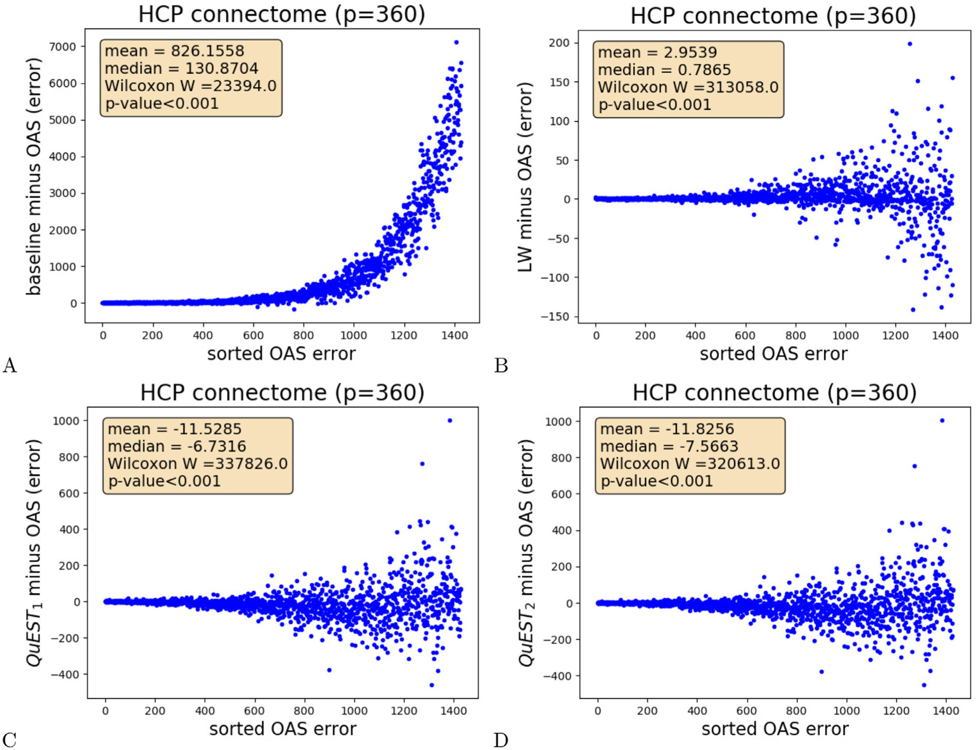
For all the high-resolution HCP connectomes, difference between the connectome errors measured: (A) before OAS shrinkage (baseline) and after OAS, (B) after Ledoit-Wolf and after OAS, (C) after QuEST1 and OAS, (D) after QuEST2 and OAS, as a function of the OAS error. The first two error differences are significantly positive (Wilcoxon sign-rank test p-values lower than 0.001, for a positive differences median). These results indicates that OAS significantly outperforms baseline and Ledoit-Wolf shrinkage. On the other hand, QuEST methods produced significantly better connectomes (Wilcoxon sign-rank test p-values lower than 0.001, for a negative differences median).
4.5. Computational time
NERCOME was the most time-consuming method, even when running for a single parameter value. NERCOME is straightforward to implement but requires multiple time-consuming matrix multiplications and additions. In addition, the method depends on a parameter, the proportion of samples retained to compute S2 during each split, which can only be selected by conducting an experimental replication or a cross-validation. This extra step of parameter selection further increases NERCOME computational cost. As a result, the computational burden was significantly larger for NERCOME than the other methods tested. The second slowest approach was QuEST, because of the cost required for the numerical inversion of the equations defined by the method. The other methods, the OAS, NAS, and the original LW method, exhibited a similar, significantly faster speed and would scale to large matrices, as noted by Ledoit and Wolf (2020).
4.6. Shrinkage alterations
The agreement between OAS and the other methods shown in Fig. 6 for the high-resolution HCP parcellation and in supplementary materials for the other networks are always larger than 0.9, the largest values been obtained with the original Ledoit-Wolf linear shrinkage and QuEST. These large Spearman correlations suggest that OAS alterations are a reliable indicator of the alterations that would be introduced by the other methods. In other words, when OAS flags connectomes as less reliable and corrects them more substantially, other shrinkage methods would introduce stronger corrections as well.
Fig. 6.

For the high-resolution HCP network, comparison between the connectome alterations introduced by the OAS and (A) Ledoit-Wolf shrinkage (LW), (B) the nonlinear analytical shrinkage method (NAS), (C) the best NERCOME method (N ERCOM E90), (D) QuEST implemented using the first solver (QuEST1), and (E) QuEST implemented using the second solver (QuEST2). In B, a few outliers were obtained when the NAS method diverged for number of time points close to the dimension of the matrix.
4.7. Thresholded connectomes
Figs. 7 and supplemental Figure 11 show that OAS has the effect of maintaining a good precision for thresholded connectomes derived from short scans. By focusing on a reduced set of reliable correlations, OAS is able to prune a significant part of the spurious connections that gradually appear in thresholded connectomes derived from empirical correlations as the number of time points is reduced. This benefit is sometimes associated with a moderate accuracy improvement, such as the one observed for the high-resolution HCP parcellation. However, it systematically comes at the cost of a reduced Jaccard Index, the shrinkage reducing the overlap between random and ground truth connectomes by strongly restricting the number of connections in random connectomes. The results obtained for the higher thresholds shown in supplementary materials indicate that these effects are stronger when the threshold is set to larger values selecting fewer connections, as long as OAS does not discard all the correlations. This issue happened once during the experiments, for connectomes estimated from 25 time points, for the high-resolution HCP parcellation, and the largest threshold tested τ = 0. 5. Interestingly, for the high-resolution HCP parcellation and the largest threshold τ, the precision improvements induced by OAS were still fairly strong for the longest time series tested: for the time series of five hundred time points, corresponding to six minutes scans acquired using the HCP protocol, the baseline precision of 0.89 was boosted by the OAS to 0.96. This corresponds to a threefold reduction of the fraction of spurious connections in the connectomes (4% versus 11%).
Fig. 7.

When connectomes are thresholded at correlations larger than 0.3 (τ = 0. 3), precision, accuracy and Jaccard index measured with and without OAS for increasing number of time points and (A) high-resolution HCP parcellation, and (B) low-resolution HCP parcellation.
4.8. Heterogeneous datasets
Fig. 8 demonstrates that, for the synthetic data generated in this experiment, OAS reduces connectome heterogeneity and produces connectomes that are not only closer to each other but also closer to the ground truth they are attempting to capture. However, the fact that all the connectomes are shrunk towards the identity matrix shifts their mean and introduces bias. This issue could perhaps be addressed in the future by developing new shrinkage methods using the population average correlation matrix as a shrinkage target (Rahim et al., 2019; Schäfer and Strimmer, 2005).
Fig. 8.

Connectivity matrix spread (spread), connectivity matrix spread around the study participant connectivity matrix (ground truth spread, GT spread), and distance between average of the connectivity matrices and the study participant average connectivity matrix (bias) measured before and after Oracle Approximating Shrinkage (OAS) for all 250 HCP study participants and (A) the high-resolution HCP parcellation, (B) the low-resolution HCP parcellatioin, (C) the DMN, (D) the DLPFC.
Fig. 9 presents the ABIDE dataset, the OAS intensity, and the proportion of pairwise functional connections strongly associated with ASD that are reinforced after OAS. These results point the variability between the 17 ABIDE acquisition sites. Most shrinkage intensities, close to 0.1 or larger, are not negligible. As a result, OAS had a noticeable impact on the results. By reinforcing the most significant associations while reducing the significance of spurious associations (see supplementary materials), OAS had a beneficial impact similar to a denoising procedure. The parcellation associated with the smallest shrinkage intensities was the Harvard-Oxford parcellation (ho, 111 parcels), followed by Eickhoff-Zilles (ez, 116 parcels), the Automated Anatomical Labeling (aal, 116 parcels), the Craddock 200 parcellation (CC200, 200 parcels), the Talaraich and Tournoux parcellation (tt, 97 parcels), and the Craddock 400 parcellation (CC400, 392 parcels). The Dosenbach 160 parcellation (do160, 161 parcels) produced the worst connectivity matrices. For all the parcellations except Dosenbach 160 the scans acquired at the Max-Mun and OHSU sites were the worst and the scans acquired at CMU, Leuven, and UM the bests. Please refer to the supplementary materials for complete results.
Fig. 9.

(A) the OAS intensity of the connectivity matrices derived from the AAL atlas strongly depend on the acquisition site, (B) OAS intensity also depends on the parcellation, (C) number of scans acquired at each location, (D) proportion of pairwise connections that differ more after OAS, between ASD and controls, among the most significantly different connections before shrinkage (the worst two parcellations are not shown). Shrinkage tends to reinforce strong ASD effects for all the parcellations.
5. Discussion
5.1. Summary
This work examined how the most prominent covariance shrinkage methods available today could be used to improve functional connectomes. The experiments were carried out on a benchmark dataset of a thousand high-resolution fMRI scans extracted from the Human Connectome Project dataset, that were used to generate thousands of short time series to study the benefits of covariance shrinkage for various scans durations. The investigations were replicated for four functional networks presenting different topologies and spatial resolutions: the entire cortex for high-resolution and low-resolution HCP parcellations, the spatially disconnected regions part of the DMN, and the functional units inside the DLPFC.
Our experimental results suggest that the connectome alterations introduced by the different methods are in agreement. When set correctly, all the methods were able to improve the connectomes derived from short fMRI time series significantly. Method comparisons suggest that NERCOME should not be used, the original Ledoit-Wolf shrinkage is obsolete compared to the OAS, and the QuEST method is the gold standard for nonlinear shrinkage approaches. The most recent approach, the nonlinear analytical method, requires additional implementation fixes. We established that shrinkage significantly improves the quality of thresholded binary connectomes (Bullmore and Sporns, 2009; Rubinov and Sporns, 2010) by pruning unreliable connections. Lastly, we found that the shrinkage intensity charts derived to investigate the effects of the OAS method are not only easy to interpret but also predictive: they delimit ranges of settings where functional connectomes cannot be correctly estimated. These charts suggest, in particular, that sparse connectomes require large numbers of time points to be distinguished from random noise. This observation is in line with the literature on sparse covariance estimation, that reports estimation errors for sparse covariance matrices slowly decreasing with the number of samples (Bien and Tibshirani, 2011), such as the EC2 method estimation error proportional to the square root of the inverse of the number of samples (Liu et al., 2014). This result is of crucial importance, as it states the impossibility of studying dynamic functional connectivity below a connectome density limit that depends on the length of the time windows considered to estimate that connectivity (Zhang et al., 2018). By reporting the characteristics of our functional networks on these charts, we found that typical connectomes derived from fMRI time series of a hundred to three hundred time points, while being relatively well estimated, would still significantly benefit from shrinkage. We observed that the best nonlinear method (QuEST) does not systematically outperform the best linear method (OAS). This result suggests that the superior flexibility of the nonlinear shrinkage methods might sometimes lead to a form of overfitting. So, we would suggest the simpler, most computationally efficient, and easier to interpret OAS method as a gold standard for fMRI processing.
5.2. Test-retest connectome reliability
Our results are in line with previous works that have established that other forms of connectivity shrinkage can successfully improve the test-retest reproducibility of correlation matrices (Mejia et al., 2018, 2015). When investigating the reliability of connectomes derived from fMRI scans, the meta-analysis (Noble et al., 2019) concluded that test-retest reproducibility increases with the amount of fMRI data available to estimate the connectomes and with the strength of their connections. These effects are consistent with our OAS intensity charts predicting better connectivity estimates for long BOLD time series and dense connectomes. However, it is still unclear how our results could be exploited to predict the reliability of individual connections as in recent works (Noble et al., 2019; Zhang et al., 2018).
5.3. Partial correlations
These test-retest studies have also pointed that partial correlations are less reliable than Pearson correlations, an issue that has already been reported multiple times in the past (Mejia et al., 2018; Noble et al., 2019; Smith et al., 2011). In the light of our results, this fact could be explained by the lower density of the connectomes derived from partial correlations, which makes them more difficult to distinguish from noisy fluctuations (Varoquaux et al., 2010). But more investigations would be required to compare the different approaches that could be employed to shrink partial correlations before concluding whether partial correlations necessarily require more shrinkage than the full Pearson correlation they originate from.
In any case, partial correlations estimation could also benefit from the covariance shrinkage methods presented in this work, particularly when the number of time points is smaller than the spatial dimension. In this setting, empirical covariance matrices are not invertible. By scaling null covariance matrix eigenvalues to strictly positive values, covariance shrinkage fixes the issue by producing an invertible matrix. A step of covariance shrinkage can thus be performed as a preprocessing before computing partial correlations via covariance matrix inversion (Varoquaux et al., 2010). By increasing the values of small noisy eigenvalues in the covariance matrix, covariance shrinkage also has the effect of reducing their influence in the precision matrices, which contributes to denoising the partial correlations (Honnorat and Davatzikos, 2017).
5.4. Binary connectomes
When binary connectomes are defined by thresholding Pearson correlations according to their amplitudes (Bullmore and Sporns, 2009; Rubinov and Sporns, 2010), the lack of data induces the apparition of spurious connections. During our experiments, the OAS was very efficient at pruning these wrong connections. For the connectomes derived from the high-resolution HCP parcellation and thresholded to focus on strong correlations larger than 0.5, this beneficial effect was still significant for time series of five hundred time points. These results demonstrate that covariance shrinkage methods have the potential to significantly improve the quality of binary graph connectomes extracted from short time series and individual fMRI scans. We hypothesize that these more reliable connectomes would exhibit more stable graph theoretical measures as well (Bullmore and Sporns, 2009; Rubinov and Sporns, 2010).
5.5. Dynamic functional connectivity
We think that our results bear crucial implications for dynamic functional connectivity (dFC) studies. Covariance shrinkage mitigates a form of statistical noise introduced by the limited ability of empirical Pearson correlations to capture exact Pearson correlation values when data lacks for the estimation. In dFC studies where Pearson correlations are computed for short time windows, this statistical noise will amount for a significant part of the dFC variability. As a result, all the statistics derived from dFC, such as standard deviation, ALFF, and excursion (Zhang et al., 2018) will be corrupted by a noise that has no biological substrate of interest. This issue calls for caution when conducting dFC studies and analyzing their results.
5.6. Scan duration and target networks
Lastly, we think that our OAS intensity charts could help designing fMRI experiments. Scan duration is a highly debated question in the field. Most researchers agree that longer scanning times produce more accurate results but resources are limited and the scanners could be employed to acquire other MRI modalities (Anderson et al., 2011; Birn et al., 2013; Dijk et al., 2010; Gonzalez-Castillo et al., 2014; Noble et al., 2019; Shehzad et al., 2009). While preliminary works had initially concluded that a duration of five to ten minutes was sufficient to acquire resting-state fMRI scans (Dijk et al., 2010; Shehzad et al., 2009) subsequent studies established that test-retest reproducibility is significantly better for half-hour-long scans and that the functional features derived for individual study participants known as functional fingerprints can improve up to a cumulated scan duration of four hours (Anderson et al., 2011; Birn et al., 2013; Gonzalez-Castillo et al., 2014). Our results indicate that the number of BOLD measurements required to achieve a target OAS shrinkage intensity depends on the density of the functional networks under investigation and its number of nodes. Once that density has been obtained, for instance, by running a pilot data acquisition, our charts could be used to select a minimal scan duration ensuring that the statistical estimates of all the functional networks investigated in the study are of sufficient quality.
For instance, the charts of Fig. 3 indicate that for the low-resolution HCP connectome one hundred fifty BOLD measurements are necessary to reach an average OAS intensity close to 0.1, corresponding to an overall error on empirical Pearson correlations amplitude around 10%. For the high-resolution HCP connectome, two hundred fifty measurements are required to reach the same quality. As a result, the ADNI3 protocol, that consists in acquiring ten-minutes-long scans at TR 3 seconds and produces scans with 200 time points Alzheimer’s Disease Neuro Imaging III (ADNI3), would only be sufficient for studying the impact of aging and neurodegenerative diseases on the low-resolution HCP connectome, that describes the functional connectivity between 44 large brain regions. By contrast, concatenating the two scans acquired for each participant of the preventAD study (304 seconds per scan, TR 2 seconds) would provide enough measurements to study as well, in that cohort, the impact of Alzheimer’s Disease on the high-resolution functional connectome that captures the connectivity between 360 fine brain parcels (Tremblay-Mercier et al., 2021).
Our results also suggest that the new scanning procedures with short TR, such as multi-band acquisitions (Feinberg and Setsompop, 2013; Moeller et al., 2010; Smitha et al., 2018), should improve functional connectivity estimates by providing more temporal measurements for similar scan duration. As long as the artifacts introduced during these acquisitions are maintained at a negligible level (Risk et al., 2021) and as long as increasing temporal resolution brings useful information for the estimation of BOLD fluctuations within the frequency range of 0.1 to 0.01 Hz commonly selected to study functional connectivity (Zou et al., 2008), an improved temporal resolution should, in theory, better capture the functional networks that are currently well measured and allow for the exploration of sparse networks more difficult to capture.
5.7. Limitations
The covariance shrinkage methods used in this work assume that the BOLD measures were statistically independent in time. This assumption might not hold in practice for time series acquired at very small repetition times. In general, the information contained in BOLD time series could be lower than expected, in the presence of repeated measurements or due to scrubbing (Power et al., 2014). As a result, we think that the methods studied in this work are only providing an upper bound of the connectome quality: poorly estimated connectomes flagged by shrinkage methods might be even more corrupted in practice. In the future, the use of statistical methods factoring out redundancies in BOLD time series to compress them to an effective duration better reflecting their underlying information might fix this limitation.
6. Conclusion
In this article, we used a thousand high-resolution fMRI scans from the Human Connectome Project to compare the ability of five prominent covariance shrinkage methods to improve the quality of functional connectomes. We established that OAS and QuEST were the best methods and NERCOME performed poorly, OAS intensity strongly depends on the density of the correlation matrices and the number of samples used to compute them but not so much on their dimension, OAS intensity is a reliable indicator of the amplitude of the correction that other shrinkage methods would introduce, sparse connectomes are difficult to estimate from short fMRI scans, shrinkage methods efficiently prune spurious connectivity in thresholded connectomes, and shrinkage would impact most standard fMRI scans and be of crucial importance for dynamic connectivity studies. We have shown how shrinkage can reduce the variability in datasets with heterogeneous scans duration. Lastly, by deriving OAS intensity charts, we provided a tool to estimate the reliability of functional connectomes. These charts could be of great help when designing and analyzing fMRI experiments and, in particular, when conducting dynamic connectivity studies.
Supplementary Material
Acknowledgments
This work has been funded in part by the National Institute of Health (NIH) grant number P30AG066546 (South Texas Alzheimer’s Disease Research Center). Data were provided by the Human Connectome Project, WU-Minn Consortium (Principal Investigators: David Van Essen and Kamil Ugurbil; 1U54MH091657) funded by the 16 NIH Institutes and Centers that support the NIH Blueprint for Neuroscience Research; and by the McDonnell Center for Systems Neuroscience at Washington University.
Footnotes
Declaration of Competing Interest
The authors declare that they have no known competing financial interests or personal relationships that could have appeared to influence the work reported in this paper.
Credit authorship contribution statement
Nicolas Honnorat: Conceptualization, Methodology, Formal analysis, Writing – original draft, Writing – review & editing. Mohamad Habes: Supervision, Writing – original draft, Writing – review & editing, Funding acquisition.
Supplementary material
Supplementary material associated with this article can be found, in the online version, at doi: 10.1016/j.neuroimage.2022.119229
Data and code availability statement
The data were provided by the HCP consortium (https://www.humanconnectome.org) and the ABIDE consortium (http://preprocessed-connectomes-project.org/abide/index.html). The nlshrink library (version 1.0.1, https://cran.r-project.org/web/packages/nlshrink/index.html) was the only external covariance shrinkage method package used in this work. All the other methods were either re-implemented or specifically developed during this project. A clean copy of these methods is freely available under a MIT licence in the following GitHub repository: https://github.com/UTHSCSA-NAL/shrinkage.
References
- Abadir K, Distaso W, Žikeš F, 2014. Design-free estimation of variance matrices. J Econom 181 (2), 165–180. [Google Scholar]
- Alzheimer’s Disease Neuro Imaging III (ADNI3) MRI Analysis User Document, 2021. Accessed December 6, 2021. http://adni.loni.usc.edu/wp-content/themes/freshnews-dev-v2/documents/mri/ADNI3_MRI_Analysis_Manual_20180202.pdf.
- Anderson JS, Ferguson MA, Larson ML, Todd DY, 2011. Reproducibility of single–subject functional connectivity measurements. American Journal of Neuroradiology 32 (3), 548–555. [DOI] [PMC free article] [PubMed] [Google Scholar]
- Bien J, Tibshirani R, 2011. Sparse estimation of a covariance matrix. Biometrika 98 (4), 807–820. [DOI] [PMC free article] [PubMed] [Google Scholar]
- Birn R, Molloy E, Patriat R, Parker T, Meier T, Kirk G, Nair V, Meyerand M, Prabhakaran V, 2013. The effect of scan length on the reliability of resting-state fMRI connectivity estimates. Neuroimage 83, 550–558. [DOI] [PMC free article] [PubMed] [Google Scholar]
- Buckner RL, Andrews-Hanna JR, Schacter DL, 2008. The brain’s default network, anatomy, function, and relevance to disease. Ann. N. Y. Acad. Sci 1–38. [DOI] [PubMed] [Google Scholar]
- Bullmore E, Sporns O, 2009. Complex brain networks: graph theoretical analysis of structural and functional systems. Nat. Rev. Neurosci 10, 186–198. [DOI] [PubMed] [Google Scholar]
- Chang C, Glover G, 2010. Time-frequency dynamics of resting-state brain connectivity measured with fMRI. Neuroimage 50, 81–98. [DOI] [PMC free article] [PubMed] [Google Scholar]
- Chen Y, Wiesel A, Eldar Y, Hero A, 2010. Shrinkage algorithms for mmse covariance estimation. IEEE Trans. Signal Process 58 (10), 5016–5029. [Google Scholar]
- Craddock C, Benhajali Y, Chu C, Chouinard F, Evans A, Jakab A, Khundrakpam B, Lewis JD, Li Q, Milham M, Yan C, Bellec P, 2013. The neuro bureau preprocessing initiative: open sharing of preprocessed neuroimaging data and derivatives. in: Neuroinformatics 2013. [Google Scholar]
- Craddock C, Sikka S, Cheung B, Khanuja R, Ghosh S, Yan C, Li Q, Lurie D, Vogelstein J, Burns R, Colcombe S, Mennes M, Kelly C, Martino AD, Castellanos F, Milham M, 2013. Towards automated analysis of connectomes: the configurable pipeline for the analysis of connectomes (C-PAC). Front Neuroinform (42). [Google Scholar]
- Daniels M, Kass R, 2001. Shrinkage estimators for covariance matrices. Biometrics 57 (4), 1173–1184. [DOI] [PMC free article] [PubMed] [Google Scholar]
- Deligianni F, Centeno M, Carmichael D, Clayden J, 2014. Relating resting-state fMRI and EEG whole-brain connectomes across frequency bands. Front Neurosci 8, 258. [DOI] [PMC free article] [PubMed] [Google Scholar]
- Dijk KV, Hedden T, Venkataraman A, Evans K, Lazar S, Buckner R, 2010. Intrinsic functional connectivity as a tool for human connectomics: theory, properties, and optimization. J. Neurophysiol 103, 297–321. [DOI] [PMC free article] [PubMed] [Google Scholar]
- Essen DCV, Smith S, Barch D, Behrens T, Yacoub E, 2013. K. ugurbil for the WU-Minn HCP consortium., the wu-minn human connectome project: an overview. Neuroimage 80, 62–79. [DOI] [PMC free article] [PubMed] [Google Scholar]
- Feinberg D, Setsompop K, 2013. Ultra-fast mri of the human brain with simultaneous multi-slice imaging. J. Magn. Reson 229, 90–100. [DOI] [PMC free article] [PubMed] [Google Scholar]
- Fox M, Raichle ME, 2007. Spontaneous fluctuations in brain activity observed with functional magnetic resonance imaging. Nat. Rev. Neurosci 8, 700–711. [DOI] [PubMed] [Google Scholar]
- Fritsch V, Varoquaux G, Thyreau B, Poline J, Thirion B, 2012. Detecting outliers in high-dimensional neuroimaging datasets with robust covariance estimator. Med Image Anal 16, 1359–1370. [DOI] [PubMed] [Google Scholar]
- Glasser M, Coalson T, Robinson E, Hacker C, Harwell J, Yacoub E, Ugurbil K, Andersson J, Beckmann C, Jenkinson M, Smith S, Essen DV, 2016. A multi-modal parcellation of human cerebral cortex. Nature 536, 171–178. [DOI] [PMC free article] [PubMed] [Google Scholar]
- Glasser S, Wilson C, Fischl A, Xu J, Webster P, Van Essen J, 2013. Neuroimage. The minimal preprocessing pipelines for the Human Connectome Project 80, 105–124. [DOI] [PMC free article] [PubMed] [Google Scholar]
- Gonzalez-Castillo J, Handwerker DA, Robinson ME, Hoy CW, Buchanan LC, Saad ZS, Bandettini PA, 2014. The spatial structure of resting state connectivity stability on the scale of minutes. Front Neurosci 8 (138). [DOI] [PMC free article] [PubMed] [Google Scholar]
- Honnorat N, Davatzikos C, 2017. Riccati-regularized Precision Matrices for Neuroimaging. In: Information Processing in Medical Imaging (IPMI), pp. 275–286. [DOI] [PMC free article] [PubMed] [Google Scholar]
- Lam C, 2016. Nonparametric eigenvalue-regularized precision or covariance matrix estimator. The Annals of Statistics 44 (3), 928–953. [Google Scholar]
- Ledoit O, Wolf M, 2003. Improved estimation of the covariance matrix of stock returns with an application to portfolio selection. Journal of Empirical Finance 10 (5), 603–621. [Google Scholar]
- Ledoit O, Wolf M, 2004. A well-conditioned estimator for large-dimensional covariance matrices. J Multivar Anal 88 (2), 365–411. [Google Scholar]
- Ledoit O, Wolf M, 2012. Nonlinear shrinkage estimation of large-dimensional covariance matrices. Ann Stat 40 (2), 1024–1060. [Google Scholar]
- Ledoit O, Wolf M, 2015. Spectrum estimation: a unified framework for covariance matrix estimation and pca in large dimensions. J Multivar Anal 139 (2), 360–384. [Google Scholar]
- Ledoit O, Wolf M, 2017. Numerical implementation of the quest function. Computational Statistics & Data Analysis 115, 199–223. [Google Scholar]
- Ledoit O, Wolf M, 2020. Analytical nonlinear shrinkage of large-dimensional covariance matrices. The Annals of Statistics 48 (5), 3043–3065. [Google Scholar]
- Liu H, Wang L, Zhao T, 2014. Sparse covariance matrix estimation with eigenvalue constraints. Journal of computational and graphical statistics 23 (2), 439–459. [DOI] [PMC free article] [PubMed] [Google Scholar]
- Martino AD, Yan C, Li Q, Denio E, Castellanos FX, Alaerts K, Anderson J, Assaf M, Bookheimer S, Dapretto M, Deen B, Delmonte S, Dinstein I, Ertl-Wagner B, Fair D, Gallagher L, Kennedy DP, Keown CL, Keysers C, Lainhart J, Lord C, Luna B, Menon V, Minshew N, Monk C, Mueller S, Müller R-A, Nebel M, Nigg J, O’Hearn K, Pelphrey K, Peltier S, Rudie J, Sunaert S, Thioux M, Tyszka J, Uddin L, Verhoeven J, Wenderoth N, Wiggins J, Mostofsky S, Milham M, 2014. The autism brain imaging data exchange: towards a large-scale evaluation of the intrinsic brain architecture in autism. Mol. Psychiatry 19 (6), 659–667. [DOI] [PMC free article] [PubMed] [Google Scholar]
- Mejia A, Nebel M, Barber A, Choe A, Pekar B, Caffo J.J.a., Lindquist M, 2018. Improved estimation of subject-level functional connectivity using full and partial correlation with empirical bayes shrinkage. Neuroimage 478–491. [DOI] [PMC free article] [PubMed] [Google Scholar]
- Mejia A, Nebel M, Shou H, Crainiceanu C, Pekar J, Mostofsky S, Caffo B, Lindquist M, 2015. Improving reliability of subject-level resting-state fMRI parcellation with shrinkage estimators. Neuroimage (112) 14–29. [DOI] [PMC free article] [PubMed] [Google Scholar]
- Moeller S, Yacoub E, Olman C, Auerbach E, Strupp J, Harel N, U ğurbil K, 2010. Multiband multislice GE-EPI at 7 tesla, with 16-fold acceleration using partial parallel imaging with application to high spatial and temporal whole-brain fMRI. Magn Reson Med 63 (5), 1144–1153. [DOI] [PMC free article] [PubMed] [Google Scholar]
- Ng B, Abugharbieh R, Varoquaux G, Poline J, Thirion B, 2011. Connectivity-informed fMRI Activation Detection. In: Medical Image Computing and Computer-Assisted Intervention (MICCAI), pp. 285–292. [DOI] [PubMed] [Google Scholar]
- Ng B, Varoquaux G, Poline J, Thirion B, 2012. A Novel Sparse Graphical Approach for Multimodal Brain Connectivity Inference. Medical Image Computing and Computer-Assisted Intervention (MICCAI). [DOI] [PubMed] [Google Scholar]
- Ng B, Varoquaux G, Poline J, Thirion B, 2013. A Novel Sparse Group Gaussian Graphical Model for Functional Connectivity Estimation. Information Processing in Medical Imaging (IPMI). [DOI] [PubMed] [Google Scholar]
- Noble S, Scheinost D, Constable R, 2019. A decade of test-retest reliability of functional connectivity: a systematic review and meta-analysis. Neuroimage 203, 11615. [DOI] [PMC free article] [PubMed] [Google Scholar]
- Power J, Mitra A, Laumann T, Snyder A, Schlaggar B, Petersen S, 2014. Methods to detect, characterize, and remove motion artifact in resting state fMRI. Neuroimage 84, 320–341. [DOI] [PMC free article] [PubMed] [Google Scholar]
- Rahim M, Thirion B, Varoquaux G, 2019. Population shrinkage of covariance (posce) for better individual brain functional-connectivity estimation. Med Image Anal 54, 138–148. [DOI] [PubMed] [Google Scholar]
- Rajaratnam B, Vincenzi D, 2016. A theoretical study of stein’s covariance estimator. Biometrika 103 (3), 653–666. [Google Scholar]
- Risk B, Murden R, Wu J, Nebel M, Venkataraman A, Zhang Z, Qiu D, 2021. Which multiband factor should you choose for your resting-state fMRI study? Neuroimage 234, 117965. [DOI] [PMC free article] [PubMed] [Google Scholar]
- Rubinov M, Sporns O, 2010. Complex network measures of brain connectivity: uses and interpretations. Neuroimage 52 (3), 1059–1069. [DOI] [PubMed] [Google Scholar]
- Schäfer J, Strimmer K, 2005. A shrinkage approach to large-scale covariance matrix estimation and implications for functional genomics. Stat Appl Genet Mol Biol 4 (1), 32. [DOI] [PubMed] [Google Scholar]
- Shehzad Z, Kelly A, Reiss P, Gee D, Gotimer K, Uddin L, Lee S, Margulies D, Roy A, Biswal B, Petkova E, Castellanos F, Milham M, 2009. The resting brain: unconstrained yet reliable. Cerebral Cortex 19, 2209–2229. [DOI] [PMC free article] [PubMed] [Google Scholar]
- Smith SM, Miller KL, Salimi-Khorshidi G, Webster M, Beckmann CF, Nichols TE, Ramsey JD, Woolrich MW, 2011. Network modelling methods for fMRI. Neuroimage 54, 875–891. [DOI] [PubMed] [Google Scholar]
- Smitha K, Arun K, Rajesh P, Joel S, Venkatesan R, Thomas B, Kesavadas C, 2018. Multiband fmri as a plausible, time-saving technique for resting-state data acquisition: study on functional connectivity mapping using graph theoretical measures. Magn Reson Imaging 53, 1–6. [DOI] [PubMed] [Google Scholar]
- Stein C, 1975. Estimation of a Covariance Matrix, Rietz Lecture. 39th Annual Meeting IMS, Atlanta, Georgia. [Google Scholar]
- Stein C, 1986. Lectures on the theory of estimation of many parameters. Journal of Mathematical Sciences 1 (34), 1373–1403. [Google Scholar]
- Stokes P, Purdon P, 2017. A study of problems encountered in granger causality analysis from a neuroscience perspective. Proceedings of the National Academy of Sciences of the United States of America (PNAS) 114 (34). E7063–E7072 [DOI] [PMC free article] [PubMed] [Google Scholar]
- Tremblay-Mercier J, Madjar C, Das S, Binette AP, Dyke S, Étienne P, Lafaille-Magnan M, Remz J, Bellec P, Collins DL, Rajah MN, Bohbot V, Leoutsakos J, Iturria-Medina Y, Kat J, Hoge R, Gauthier S, Tardif C, Chakravarty MM, Poline J, Rosa-Neto P, Evans A, Villeneuve S, Poirier J, Breitner J, 2021. Open science datasets from prevent-ad, a longitudinal cohort of pre-symptomatic alzheimer’s disease. NeuroImage Clinical 31, 102733. [DOI] [PMC free article] [PubMed] [Google Scholar]
- Varoquaux G, Gramfort A, Poline J, Thirion B, 2010. Brain Covariance Selection: Better Individual Functional Connectivity Models Using Population Prior. Advances in Neural Information Processing Systems. [Google Scholar]
- WU-Minn HCP 1200 Subjects Data Release: Reference manual, updated April 10, 2018. Accessed July 7, 2021 (March 2017).
- Zhang C, Baum S, Adduru V, Biswal B, Michael A, 2018. Test-retest reliability of dynamic functional connectivity in resting state fMRI. Neuroimage 183, 907–918. [DOI] [PubMed] [Google Scholar]
- Zou Q, Zhu C, Yang Y, Zuo X-N, Long X-Y, Cao Q-J, Wang Y-F, Zang YF, 2008. An improved approach to detection of amplitude of low-frequency fluctuation (alff) for resting-state fmri: fractional alff. J. Neurosci. Methods 172 (1), 137–141. [DOI] [PMC free article] [PubMed] [Google Scholar]
Associated Data
This section collects any data citations, data availability statements, or supplementary materials included in this article.
Supplementary Materials
Data Availability Statement
The data were provided by the HCP consortium (https://www.humanconnectome.org) and the ABIDE consortium (http://preprocessed-connectomes-project.org/abide/index.html). The nlshrink library (version 1.0.1, https://cran.r-project.org/web/packages/nlshrink/index.html) was the only external covariance shrinkage method package used in this work. All the other methods were either re-implemented or specifically developed during this project. A clean copy of these methods is freely available under a MIT licence in the following GitHub repository: https://github.com/UTHSCSA-NAL/shrinkage.