Introduction of an artificial neural network–based method for concentration‐time predictions

Abstract

Pharmacometrics and the application of population pharmacokinetic (PK) modeling play a crucial role in clinical pharmacology. These methods, which describe data with well‐defined equations and estimate physiologically interpretable parameters, have not changed substantially during the past decades. Although the methods have proven their usefulness, they are often resource intensive and require a high level of expertise. We investigated whether a method based on artificial neural networks (ANNs) may provide an alternative approach for the prediction of concentration‐time curve to supplement the gold standard methods. In this work, we used simulated data to overcome the requirement for a large clinical training data set, implemented a pharmacologically reasonable network architecture to improve extrapolation to different dosing schemes, and used transfer learning to quickly adapt the predictions to new patient groups. We demonstrate that ANNs are able to learn the shape of concentration‐time curves and make individual predictions based on a short sequence of PK measurements. Furthermore, an ANN trained on simulated data was applied to real clinical data and was demonstrated to extrapolate to different dosing schemes. We also adapted the ANN trained on simulated healthy subjects to simulated hepatic impaired patients through transfer learning. In summary, we demonstrate how ANNs could be leveraged in a PK workflow to efficiently make individual concentration‐time predictions, and we discuss the current limitations and advantages of such an ANN‐based method.

Study Highlights.

WHAT IS THE CURRENT KNOWLEDGE ON THE TOPIC?

The current state of the art for pharmacokinetic (PK) modeling and prediction is based on well‐defined mathematical models usually using ordinary differential equation (ODE)–based methods.

WHAT QUESTION DID THIS STUDY ADDRESS?

This work investigates whether artificial neural networks (ANNs) can be used to make PK predictions similar to ODE‐based methods.

WHAT DOES THIS STUDY ADD TO OUR KNOWLEDGE?

We demonstrate that ANNs are able to make PK concentration predictions for which ODE‐based methods are usually used. Their ability to explore dose regimens they were not trained on showcases their possible application in precision dosing. Also, the possibility to retrain an ANN on small data sets to transfer from one patient group to another shows a beneficial property of ANNs in precision dosing.

HOW MIGHT THIS CHANGE DRUG DISCOVERY, DEVELOPMENT, AND/OR THERAPEUTICS?

ANNs provide an efficient and easy‐to‐use supplementary method to state‐of‐the‐art population PK modeling approaches and can help increase efficiency for certain applications in pharmacometrics.

INTRODUCTION

Pharmacometrics describes the field of quantitative and qualitative analyses of pharmacological data through modeling, for example, the modeling of pharmacokinetic (PK) data from a clinical study. ¹ It is an integral part in the approval of new pharmaceutical products through health authorities and a key element for personalized dosing. Although the state‐of‐the‐art methods in pharmacometrics have proven their usefulness for many years, few parts of typical workflows are automated, there is a requirement for a high level of expertise of the modeler, and there is room for improvement in terms of efficiency.

One state‐of‐the‐art approach in pharmacometrics is population PK (popPK) modeling, ² where drug concentration data are described through a structural model with well‐defined equations including physiologically interpretable parameters. This model is developed through iteratively fitting a candidate structural model, assessing its goodness of fit, identifying possible systematic residual errors, and adjusting the model accordingly. ³ In addition, quantitative relationships between individual parameters and patients' characteristics are investigated, usually through stepwise covariate modeling. Both the model development and the covariate selection require multiple rounds of parameter calibration, which may result in substantial development time. ⁴ , ⁵

PopPK modeling allows pharmacometricians to investigate clinical data, find sources of variability of drug exposure in a population, and describe these through popPK parameters and their relationships to patients' covariates. ⁶ One specific application of popPK modeling is to make concentration‐time curve predictions for an individual patient. This enables exploration of different dose regimens to find a regimen with an optimal drug exposure for a given patient.

With the increase in computational power and available data, artificial neural networks (ANNs) have gained a strong place in many fields of daily life. They are used for text completion in emails ⁷ and autonomously driving cars ⁸ and have even been introduced in the discovery of new antibiotics. ⁹ Although ANNs have not yet been widely adopted in clinical pharmacology and pharmacometrics, multiple publications point to their potential to become an important tool in these subject areas as well. ¹⁰ , ¹¹ , ¹²

In this article, we introduce the concept of ANNs to pharmacometricians, highlight their capability for concentration‐time curve predictions, and discuss their differences and limitations compared with classical methods.

METHODS

Work overview

In this work, we demonstrate how an ANN‐based method predicts PK concentration‐time curves for individual subjects, and we show how this method could be used in a clinical pharmacology setting with a limited amount of data. Figure 1 illustrates the workflow followed in this study. First, we used a physiologically based PK (PBPK) model to simulate concentration‐time profiles. We sampled from these simulated profiles at regular intervals to generate a training data set for the ANN model, and the trained ANN was then tested for its ability to capture the training data set. Second, the ANN was tested against the actual measured clinical PK data before we further investigated its ability to extrapolate to different dosing regimens. Finally, we used the PBPK model to generate data for an hepatically impaired patient population and applied transfer learning to retrain the ANN for this different patient group.

FIGURE 1.

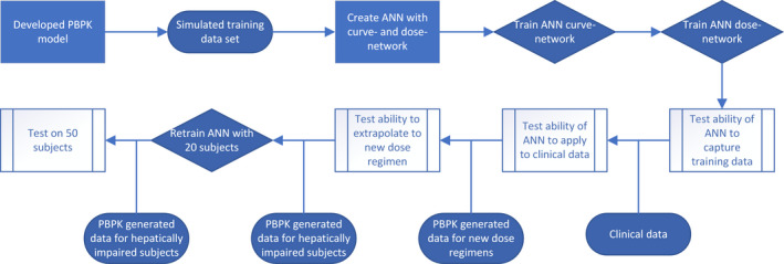
The flowchart illustrates the workflow followed in this study. A developed PBPK model is used to generate a training data set to train the ANN. The trained ANN is first tested with simulated data, followed by testing on real clinical data. In the next step, dose regimen extrapolation ability is investigated. Furthermore, the ANN is retrained on 20 hepatically impaired patients generated by the PBPK model and whether the ANN was able to retrain with a data set of this size was tested. ANN, artificial neural network; PBPK, physiologically based pharmacokinetic

Artificial neural networks

ANNs belong to the family of the supervised machine‐learning (ML) methods. ANNs are able to approximate linear and nonlinear functions by creating a network of calculation steps and calibrating the model parameters of this network to data. ¹³ For consistency, hereafter when connected to ANN, model calibration and parameters are referred to as training and weights/biases, respectively. The architecture of an ANN is structured in input, hidden, and output layers. The input layer defines which information is provided to the ANN, which in mathematical terminology corresponds to the independent variables. Pharmacometric variables that may form the input layer might include patient characteristics, measured concentrations, or combinations of different data types. The output layer represents the dependent variable, which may be a predicted outcome or the concentration at the next time step. The hidden layers define the calculation steps that lead from the input to the output layer. For different calculations and data types, different types of hidden layers can be used. Two common layer types are densely connected layers and long short‐term memory ¹⁴ (LSTM) layers. Although dense layers are used to handle static data points, LSTM layers are specifically tailored to temporal sequences of data points.

Although very simple ANNs with, for example, one hidden layer and only a few weights may be expressed as an explicit function (which is equivalent to a nonlinear regression), the strength of ANNs lies in the possibility to largely increase their complexity through increasing the number of hidden layers. With this, ANNs can approximate highly complex functions at the expense of losing comprehensibility, which is the reason why they are often referred to as a “black box” method. Although weights mathematically represent the parameters of an ANN, it is important to note that the weights and biases of a neural network do not represent physiologically or pharmacokinetically meaningful parameters but, rather, are comparable with parameters from a regression model.

ANN training

A training data set can be used to calibrate the weights of an ANN. ¹⁵ This training data set requires output data for each input data. To make useful predictions, the training data should be representative for the setting in which an ANN is applied. The weights of an ANN are adjusted during training, usually using a gradient‐based method, to minimize a loss/objective function assessing the difference between predicted and observed outputs. With an increasing number of hidden layers and parameters to calibrate, an increased training data set is required to manage the risk of overfitting.

Transfer learning

If the available data set for a specific problem is not large enough, the concept of transfer learning can be used. ¹⁶ An ANN previously trained on a similar but not identical problem can be retrained on a new data set. Because the previously trained ANN already learned to accomplish a similar task, some of the weights do not need to be adjusted and can be fixed for the retraining. The reduced number of adjustable weights requires a smaller data set for the retraining compared with the initial training.

ANN architecture

In PK models, dosing events manifest in abrupt changes of the system dynamics (e.g., steps in plasma profiles for intravenous dosing or discontinuous first derivatives of plasma profiles for oral dosing). The ANN we illustrate in this work predicts concentration‐time profiles at times with and without dosing events. Therefore, we structured the network architecture into two subnetworks. One subnetwork, later referred to as the curve network, is used to describe the concentration at a timepoint when no dose is administered. The other subnetwork, the dose network, is used to describe the concentration increase following a dosing event.

The input to the curve network is a concentration‐time profile (sequence), and the output is the next concentration in this sequence. The curve network is composed of two hidden LSTM layers that decompose a concentration sequence into parameters representing the shape of the sequence (Figure S1). In a subsequent densely connected layer, these parameters are used in a nonlinear combination to predict the concentration at the next time step. The input to the dose network is a concentration sequence including the peak concentration from the first dosing and the dosing sequence with the doses at each timepoint relative to the first dose. Both inputs are processed with two hidden LSTM layers and one densely connected layer. The vectors resulting from the densely connected layers were concatenated and processed with three additional densely connected layers. This architecture allows the dose network to draw a connection between a dose and the concentration increase after a dose in individual patients. The output of the dose network was added to the output of the curve network (Figure S2).

Training data

To train the ANN, we used simulated data from a PBPK model published by Parrott et al. ¹⁷ Single‐dose simulations were performed for three different dose levels and for multiple doses, and data were generated for subjects with each receiving 10 administrations of the same dose in a dosing interval of 24 h (for more details, see Table S1). Concentrations were sampled from these simulated concentration‐time profiles every hour. To streamline the training of the ANN and in accordance with a usual ML workflow, we normalized the individual concentration sequences by minimum–maximum normalization. ¹⁸

Curve network training

To train the curve network, we included samples from the single‐dose and multiple‐dose data and split them into sequences of different lengths. The multiple‐dose data was split such that for each sequence the last dosing was at least 10 h before the end of the sequence to avoid capturing dosing effects in the curve network, which may be adjusted for drugs with different absorption profiles (Figure S3c). The number of individual sequences generated through this procedure was shown to cover the variability in the training data set. We added a normally distributed proportional error with a mean of 0 and a standard deviation of 0.1 to all sequences and used them as input for the curve network. As target output for the training, we used the concentration one step forward in time relative to the last concentration in the input sequence.

We used the Adam‐optimizer ¹⁹ for parameter optimization, a standard optimizer for training ANNs, and mean squared error as the loss function.

Dose network training

To train the weights of the dose network, we trained the overall network with the weights of the curve network fixed. The multiple‐dose data were split into sequences including samples with the last concentration in the sequence located in a range up to 10 data points after a previous dosing to capture the effect of a new dose (Figure S3b). These sequences served as input to the fixed curve network. The inputs to the dose network were the concentration sequence and the dosing sequence as described in the ANN Architecture section.

Testing on simulated data

To assess the sensitivity of the ANN to different training data, 10 ANN variants were trained with 10 different seeds to assemble the random training data.

With each of these 10 ANNs, we predicted the complete concentration‐time curve for the subjects from the training data set to test whether the neural networks are able to approximate the shape of PK concentration‐time curves in general. We inspected the predicted concentrations one, 10, and 50 time steps ahead for the single‐dose data and at the trough and the peak predictions of the third, fourth, and fifth doses for the multiple‐dose data.

Testing on real clinical data

To investigate the translatability from simulated to observed clinical data, we used a data set of 53 subjects with single‐dose administration and six subjects with multiple‐dose administrations.¹⁷ Measurements from 0 to 8 h were initially selected as the input sequence. Because the concentrations in the single‐dose study were only measured at 0, 1, 2, 4, and 8 h, the concentrations at 3, 5, 6, and 7 h were estimated through logarithmic interpolation.

Starting from this input sequence with nine concentrations per subject, the concentration‐time curves up to 312 h were predicted through iteratively predicting the next concentration and appending the input sequence with the predicted value. To determine the goodness of fit, the measured concentrations were compared with the predicted values at the corresponding timepoint.

Test for extrapolation to different dose regimens

One key application for the ANN in clinical pharmacology and precision dosing is the possibility to simulate new dosing regimens. To test whether ANNs are able to extrapolate and make accurate predictions for dose regimens they were not trained on, the PBPK model was used to simulate additional data. The dose regimens for these simulations included an initial dose of 20 mg followed by 10 mg twice daily after 24 h or by 40 mg once every second day. The dosing scheme passed to the dose network was adjusted accordingly to predict the whole concentration‐time curves based on an initial concentration sequence.

Retraining on new data

A further challenge in clinical pharmacology are patient groups with different characteristics that lead to different pharmacological behaviors, for example, patients with a decreased clearance attributed to hepatic impairment. In classical pharmacometric approaches, physiologically interpretable parameters would be adjusted accordingly to represent such situations. In the ANN approaches, the parameters are not physiologically relevant, and therefore a new ANN must be trained for a new patient group. To minimize the required data, the ANN trained on the simulated data for common patients was used for transfer learning. ¹⁶ To demonstrate this functionality, the PBPK model was used to simulate a data set of patients with hepatic impairment with a decreased clearance rate compared with the original population. This data set was split such that 20 patients were used for the retraining and 50 patients were used to evaluate the retrained ANN. Because hepatic impairment is expected to have no influence on the characteristics of drug absorption, only the curve network was retrained and investigated. However, retraining the dose network would also be possible for other scenarios. During the retraining, the weights in the LSTM layers were fixed and only the weights in the dense layers were adjusted because we assumed that the LSTM layers can also describe the new curve and the main changes must be done in the nonlinear parameter combination part of the ANN.

The retrained ANN was used to predict the whole concentration‐time curve for the 50 patients in the test data set. The predicted concentrations at 10 equally distributed timepoints over the entire prediction time were investigated and compared with the true simulated concentrations.

RESULTS

ANNs can predict PK profiles in a simulated setting

The predicted concentration‐time curves of the ANNs for the simulated single‐dose and multiple‐dose data are in agreement with the simulated profiles generated using the PBPK model (Figure 2a,b). In the single‐dose scenario, the exponential elimination is correctly described, whereas in the multiple‐dose scenario, the drug accumulation and the steady state are adequately captured by the ANN. Thus, we conclude that in this setting the ANN is capable of producing representative PK time‐concentration profiles.

FIGURE 2.

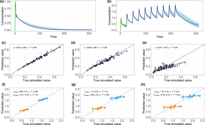
(Top) Two examples of predictions for simulated (a) single‐dose and (b) multiple‐dose data. An initial input sequence (green) was given to the 10 trained neural networks. The ranges of the artificial neural network predictions (light blue) cover the underlying simulated concentration‐time curve (dark blue line) in both of these examples. (Middle) Predictions for 100 randomly sampled simulated subjects plotted against the true simulated concentrations with the corresponding linear regression. Decreasing precision in terms of decreasing regression slope and correlation coefficients R ² was observed from (c) one‐step‐ahead predictions to (d) 10‐step‐ahead predictions and (e) 50‐step‐ahead predictions. (Bottom) Regression slope and R ² of the peak (blue triangles) and the trough predictions (orange squares) decrease from the (f) third to the (g) fourth and (h) fifth doses

The single‐dose predictions for the concentration one step ahead are very close to the simulated values (Figure 2c). With multiple iterations of predicting the next concentration and appending the input to the neural network with the prediction, the residual between the predicted value and the simulated value increases. This results in a decrease of the regression slope from 0.95 to 0.85 and 0.49 and of the correlation coefficient from 0.98 to 0.94 and 0.67 for one‐step ahead, 10‐step ahead, and 50‐step ahead predictions, respectively (Figure 2c–e). We observe the same trend for multiple doses looking at the peak and the trough predictions of the third, fourth, and fifth doses (Figure 2f–h). Interestingly, the predicted values for different subjects lay in a rather narrow range, whereas the underlying simulated values differ more from each other. This suggests an interindividual variability in the predictions that is too low.

Translation from simulated to real single‐dose data

For a similar analysis using observed clinical patient data, the range of predictions of the 10 neural networks covered the observed concentrations in most cases (Figure 3a–c). The ANNs were not only able to make good predictions for one part of the curve but also for the entire profile. The correlation between the mean predictions over all neural networks for each data point and the observed concentrations was high, with an R ² of 0.86. In the goodness‐of‐fit plot, a few outliers could be seen where the ANNs strongly underestimated the concentration. In this case, the absorption was delayed, and the peak concentration was not reached within the input sequence. Because the ANNs were trained on PK profiles with their maximum concentration within the first 9 h, they were not able to predict this outlier correctly.

FIGURE 3.

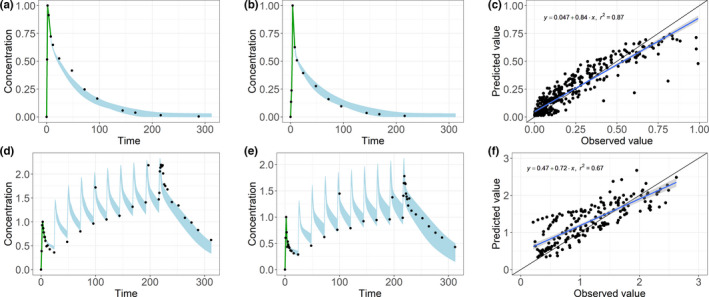
With the input sequence (green), the range in which the predictions of the 10 artificial neural networks lay (light blue) cover the majority of the observed concentrations (black dots) for two exemplary subjects with (a, b) single‐dose data and (d, e) multiple does data. The goodness‐of‐fit plots, linear regression, and correlation coefficient show a good correlation between the observed values on the x‐axis and the mean predicted values on the y‐axis for (c) single‐dose and (f) multiple‐dose predictions

Translation from simulated to real multiple‐dose data

The concentration‐time curves were predicted for a multiple‐dose schedule using the 10 neural networks (Figure 3d–f). With multiple dosing, we noted a slightly lower R ² of 0.75 compared with the single‐dose predictions. Nevertheless, the observed concentrations were within the prediction range of the neural networks for most subjects, and the ANNs were able to predict the accumulation and the steady‐state concentration.

ANNs can extrapolate to new dose regimens

The ANNs were also able to make predictions for dose regimens that were not included in the initial training data set (Figure 4). Provided with only the information on the dosing regimen, the ANN was able to capture the expected PK behavior in line with the PBPK simulations. In the high‐frequency and low‐dose regimen, we observed a smaller difference between the peak and trough concentrations, whereas in the low‐frequency and high‐dose regimen, these differences were larger compared with the original dose schedule. Also, the biphasic behavior of the high‐dose regimen was observed. There, a larger mismatch between the predicted and the underlying simulated data was observed.

FIGURE 4.

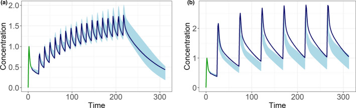
The similar input sequence (green) with the prediction range of the artificial neural networks (light blue) and the profile simulated by a physiologically based pharmacokinetic model (dark blue) for a dosing scheme with (a) a higher dosing frequency but lower doses and (b) a lower dosing frequency but higher doses show the ability of the artificial neural networks to extrapolate to different dosing schemes

ANNs can be used to predict new data without requiring a large data set

After the transfer learning with a small data set of 20 hepatically impaired patients, the ANNs clearly showed different predictions. ANN‐generated profiles after retraining were much closer to the concentration‐time curve of the hepatically impaired patients than the profiles prior to retraining (Figure 5). The mean over the predictions from 10 trained ANNs was close to the true simulated concentration, and the mean squared error decreased from 0.16 to 0.01. However, some of the individual ANNs performed less well, and the range of the predictions was larger compared with that for the nonimpaired subjects (broad range of the blue shaded area in Figure 5b).

FIGURE 5.

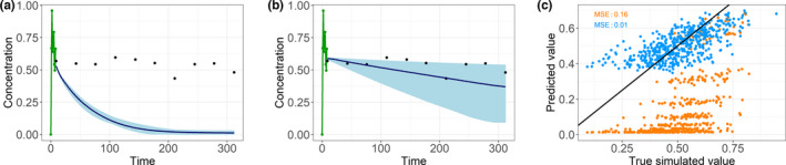
A randomly chosen patient with the input sequence (green), the range in which the predictions of the 10 artificial neural networks lay (light blue), and the mean of the predictions (dark blue) are much closer to the true simulated values (black points) after the retraining (b) compared with before the retraining (a). Also, the goodness‐of‐fit plot (c) and the corresponding mean squared errors (MSEs) show the improvement from without retraining (orange) compared to with retraining (blue)

Training and predicting efficiency

The training of the ANN was performed within 1 h on a conventional laptop (specification of computational hardware in Table S3). A prediction of a concentration‐time profile with 300 prediction steps takes <30 s. Predictions for multiple subjects can be made in parallel.

DISCUSSION

Key outcomes

The results of our study demonstrate that ANNs are able to make reasonable PK concentration‐time curve predictions without any predefined PK model. Although this study is a preliminary evaluation of this approach and extensive further evaluation is required, we consider these outcomes to be encouraging and to open further possibilities. The ANN‐based predictions shown here cannot be compared directly with the predictions of conventional population PK modeling because many of the conventional diagnostic metrics and plots are not applicable (more information in Table S2). Also, the aim and application of the two methods would not be the same. The conventional approach delivers interpretable predictions and PK parameters that allow the influence of covariates to be explored. This capability is key for individualized as well as population‐level predictions and is an established method, which is expected in support of the approval of a new drug. However, these strengths come at the cost of the required expertise and model development time. In contrast, ANN‐based predictions require only a few hours of unsupervised training. However, in the form presented here, they do not provide any rationale for the predictions and cannot be linked to PK processes or patient covariates. Although this limitation may be addressed through, for example, including patient characteristics in the input to the ANN, the current implementation might be more applicable for tasks such as the fast exploration of new data and simple extrapolations to novel dose regimens. Furthermore, the predicted concentration‐time curves could allow derivation of secondary PK parameters, such as concentration trough levels (Figure S4) or the area under the curve to have guidance for decisions. As a further key outcome of this study, we demonstrated the possibility to train an ANN on a large amount of simulated data and then retrain it on a small set of measured clinical data, thus overcoming the requirement for large clinical training data sets. This invalidates the common perception that ML methods are not available to areas of drug development where data sets are relatively small.

General discussion

In this section, the results of the study are discussed in more detail. Considering the full time‐course predictions, decreasing accuracy (lower R ² and regression slope) was observed for predictions multiple time steps ahead (Figure 2c–h). On one hand, this is probably the result of error propagation occurring when appending the input sequence with the next predicted concentration. Furthermore, the current implementation only allows training of the neural network on one‐step‐ahead predictions and therefore may be insensitive to effects of the one‐step‐ahead prediction on later timepoints. One potential solution to overcome this current limitation is to implement an alternative network architecture that would allow direct prediction of a concentration multiple timepoints ahead. A different approach that uses ANNs for similar predictions are neural ordinary differential equations (ODEs) ²⁰ as also investigated by Lu et al. ²¹ The neural ODE method combines an ANN with an ODE solver that allows predictions on an unrestricted continuous time scale. As well as these benefits, neural ODEs have some drawbacks, and the choice of method may depend on the purpose and the application.

On the other hand, the decreasing accuracy may indicate underestimation of the interindividual variability in the predictions (decreasing regression slope in Figure 2c–e and f–h). This could be addressed by basing the predictions on a combination of a concentration input sequence and some patients’ characteristics to increase the information about an individual patient provided to the ANN, which we plan to pursue in future work.

One key limitation of the current approach is the discretization of time steps as hourly sampling is not a common clinical practice. The main purpose of this densely measured input sequence is to provide information of an individual patient to the ANN. Similar information could also be given by patients’ characteristics. Providing these characteristics as an additional input to the ANN would allow for a shorter input sequence and reduce the need for a long, densely measured input sequence. Using neural ODEs as mentioned previously may be another approach to address this problem.

Another limitation is that the current curve network is averaging across dose levels and therefore does not allow adjustments for dose effects such as solubility effects or saturable absorptions. This limitation could be overcome by providing the dose as input to the curve network.

The results of the predictions for real data demonstrate the feasibility of training a neural network on simulated PK data and applying it to real clinical data. In this example, we used a PBPK model that had previously been shown to successfully simulate observed clinical data, and as a result the transition from simulated to observed data was feasible without any additional refinements of the ANN. PBPK models are often developed preclinically prior to clinical studies and could therefore be used to train a preliminary ANN before retraining with the first clinical data. There is even the prospect that a generic ANN could be trained on a large data set containing simulated data from multiple generic PK models capturing generic PK behaviors, before retraining with drug‐specific data. Such speculations will require further investigation of transfer learning, ¹⁶ which was used in this study to adjust the ANN to a different patient group but might also provide solutions for different challenges.

Possible applications

To illustrate possible applications of this approach, we present the following hypothetical scenario: prior to the first clinical study with a new molecular entity, the clinical pharmacologist (CP) needs to design phase I studies for single‐ascending and multiple‐ascending doses. A PBPK model exists that leverages all preclinical data and allows predictions of PK profiles; however, this requires a specialized PBPK modeler to run simulations to project exposures for the starting dose for single‐ascending dose studies and likely maximum dose. With a previously trained ANN, the CP could perform this task independently. Then when first clinical PK are measured after single doses, an ANN that was previously trained on PBPK data could be retrained on the clinical data to refine the multiple‐ascending dose study doses. By simply uploading the new data, the CP could apply the ANN to this task on their own within a short time frame.

CONFLICT OF INTEREST

The authors declared no competing interests for this work.

AUTHOR CONTRIBUTIONS

D.S.B., L.H., B.S., and N.P. wrote the manuscript. D.S.B., L.H., B.S., and N.P. designed the research. D.S.B., L.H., and B.S. performed the research. D.S.B., L.H., and B.S. analyzed the data.

Supporting information

Appendix S1

Appendix S2

Figure S1

Figure S2

Figure S3

Figure S4

Table S1

Table S2

Table S3

Bräm DS, Parrott N, Hutchinson L, Steiert B. Introduction of an artificial neural network–based method for concentration‐time predictions. CPT Pharmacometrics Syst Pharmacol. 2022;11:745–754. doi: 10.1002/psp4.12786

REFERENCES

- 1. Barrett JS, Fossler MJ, Cadieu KD, Gastonguay MR. Pharmacometrics: a multidisciplinary field to facilitate critical thinking in drug development and translational research settings. J Clin Pharmacol. 2008;48:632‐649. doi: 10.1177/0091270008315318 [DOI] [PubMed] [Google Scholar]
- 2. Mould DR, Upton RN. Basic concepts in population modeling, simulation, and model‐based drug development. CPT Pharmacometrics Syst Pharmacol. 2012;1:1‐14. doi: 10.1038/psp.2012.4 [DOI] [PMC free article] [PubMed] [Google Scholar]
- 3. Byon W, Smith MK, Chan P, et al. Establishing best practices and guidance in population modeling: an experience with an internal population pharmacokinetic analysis guidance. CPT Pharmacometrics Syst Pharmacol. 2013;2:1‐8. doi: 10.1038/psp.2013.26 [DOI] [PMC free article] [PubMed] [Google Scholar]
- 4. Wahlby U, Jonsson EN, Karlsson MO. Comparison of stepwise covariate model building strategies in population pharmacokinetic‐pharmacodynamic analysis. AAPS PharmSci. 2002;4:68‐79. doi: 10.1208/ps040427 [DOI] [PMC free article] [PubMed] [Google Scholar]
- 5. Smith G. Step away from stepwise. J Big Data. 2018;5:1‐12. doi: 10.1186/s40537-018-0143-6 [DOI] [Google Scholar]
- 6. Mould DR, Upton RN. Basic concepts in population modeling, simulation, and model‐based drug development – part 2: introduction to pharmacokinetic modeling methods. CPT Pharmacometrics Syst Pharmacol. 2013;2:1‐12. doi: 10.1038/psp.2013.14 [DOI] [PMC free article] [PubMed] [Google Scholar]
- 7. Chen MX, Lee B, Bansal G. Gmail smart compose: real‐time assisted writing. 2019. In Proc. ACM SIGKDD Int. Conf. Knowl. Discov. Data Min. doi: 10.1145/3292500.3330723 [DOI]
- 8. Jana S, Tian Y, Pei K, Ray B. DeepTest: automated testing of deep‐neural‐network‐driven autonomous cars. 2018. In Proc. – Int. Conf. Softw. Eng. 10.1145/3180155.3180220 [DOI]
- 9. Stokes JM, Yang K, Swanson K, et al. A deep learning approach to antibiotic discovery. Cell. 2020;180:688‐702.e13. doi: 10.1016/j.cell.2020.01.021 [DOI] [PMC free article] [PubMed] [Google Scholar]
- 10. Koch G, Pfister M, Daunhawer I, Wilbaux M, Wellmann S, Vogt JE. Pharmacometrics and machine learning partner to advance clinical data analysis. Clin Pharmacol Ther. 2020;107:926‐933. doi: 10.1002/cpt.1774 [DOI] [PMC free article] [PubMed] [Google Scholar]
- 11. Hutchinson L, Steiert B, Soubret A, et al. Models and machines: how deep learning will take clinical pharmacology to the next level. CPT Pharmacometrics Syst Pharmacol. 2019;8:131‐134. doi: 10.1002/psp4.12377 [DOI] [PMC free article] [PubMed] [Google Scholar]
- 12. McComb M, Bies R, Ramanathan M. Machine learning in pharmacometrics: opportunities and challenges. Br J Clin Pharmacol. 2021;88:1482‐1499. doi: 10.1111/bcp.14801 [DOI] [PubMed] [Google Scholar]
- 13. Hornik K, Stinchcombe M, White H. Multilayer feedforward networks are universal approximators. Neural Netw. 1989;2:359‐366. doi: 10.1016/0893-6080(89)90020-8 [DOI] [Google Scholar]
- 14. Hochreiter S, Schmidhuber J. Long short‐term memory. Neural Comput. 1997;9:1735‐1780. doi: 10.1162/neco.1997.9.8.1735 [DOI] [PubMed] [Google Scholar]
- 15. Kavzoglu T. Determining optimum structure for artificial neural networks. 1999. Proceddings 25th Annu. Tech. Conf. Exhib. Remote Sens. Soc.
- 16. Weiss K, Khoshgoftaar TM, Wang DD. A survey of transfer learning. J Big Data. 2016;3:1‐40. doi: 10.1186/s40537-016-0043-6 [DOI] [Google Scholar]
- 17. Parrott N, Hainzl D, Alberati D, et al. Physiologically based pharmacokinetic modelling to predict single‐ and multiple‐dose human pharmacokinetics of bitopertin. Clin Pharmacokinet. 2013;52:673‐683. doi: 10.1007/s40262-013-0061-x [DOI] [PubMed] [Google Scholar]
- 18. Nayak SC, Misra BB, Behera HS. Impact of data normalization on stock index forecasting. Int J Comput Inf Syst Ind Manag Appl. 2014;6:257‐269. [Google Scholar]
- 19. Kingma DP, Ba JL. Adam: a method for stochastic optimization. 2015. In 3rd Int. Conf. Learn. Represent. ICLR 2015 – Conf. Track Proc.
- 20. Chen RTQ, Rubanova Y, Bettencourt J, Duvenaud D. Neural ordinary differential equations. arXiv. 2018.
- 21. Lu J, Bender B, Jin JY, Guan Y. Deep learning prediction of patient response time course from early data via neural‐pharmacokinetic/pharmacodynamic modelling. Nat Mach Intell. 2021;3:696‐704. doi: 10.1038/s42256-021-00357-4 [DOI] [Google Scholar]
Associated Data
This section collects any data citations, data availability statements, or supplementary materials included in this article.
Supplementary Materials