Microsimulation model calibration with approximate Bayesian computation in R: A tutorial

Abstract

Mathematical health policy models, including microsimulation models (MSMs), are widely used to simulate complex processes and predict outcomes consistent with available data. Calibration is a method to estimate parameter values such that model predictions are similar to observed outcomes of interest. Bayesian calibration methods are popular among the available calibration techniques, given their strong theoretical basis and flexibility to incorporate prior beliefs and draw values from the posterior distribution of model parameters, and hence the ability to characterize and evaluate parameter uncertainty in the model outcomes. Approximate Bayesian computation (ABC) is an approach to calibrate complex models where the likelihood is intractable, focusing on measuring the difference between the simulated model predictions and outcomes of interest in observed data. While ABC methods are increasingly being used, there is limited practical guidance in the medical decision making literature on approaches to implement ABC to calibrate MSMs. In this tutorial we describe the Bayesian calibration framework, introduce the ABC approach, and provide a step-by-step guidance for implementing an ABC algorithm to calibrate MSMs, using two case examples based on a microsimulation model for dementia. We also provide the R code for applying these methods.

1. INTRODUCTION

Microsimulation models (MSMs) perform simulations at the level of the individual.¹ MSMs involve numerous parameters which dictate individual trajectories. Some MSM parameters can be directly estimated or obtained from the literature; however, often MSMs incorporate parameters that can not be directly estimated. Even when parameters are directly estimated or obtained from the literature, the MSM may yield predictions that differ from reference quantities of interest.²

Calibration is a method to estimate parameter value(s) such that model predictions are similar to observed pre-specified outcomes of interest called (calibration targets), with similarity defined by a distance function.^3,4 Consider a simple model with one parameter p, the probability of a patient dying each monthly cycle. Although p is not observed, an observational study provides an estimated mean survival time for N patients. Calibration methods use the mean survival time from the observational study in conjunction with the pre-specified calibration target(s) to find values for the parameter p. The result of the calibration procedure is a set of values for p such that the difference between model predicted survival time (model output) and the survival time (calibration target) in the observational study is minimized.

Bayesian calibration produces a distribution of acceptable values for each calibrated parameter by combining prior information with observed data to estimate the posterior distributions of calibrated model parameters.^5,6 Although Bayesian calibration can be more computationally intensive than other calibration methods, it has a strong theoretical basis and provides useful information for conveying parameter uncertainty and for conducting uncertainty analyses.^5,7,8 For MSMs, likelihood functions are often difficult or impossible to specify or simulate.⁹ Approximate Bayesian computation (ABC) is a Bayesian approach that avoids computation of the likelihood by instead measuring the difference between the simulation model’s predictions and outcomes of interest observed from available data.^10,11,12

ABC methods are increasingly being used to calibrate health policy models.¹² Although there are excellent tutorials on Bayesian calibration (e.g., see Menzies et al.)¹³, there is limited practical guidance in the literature on how to implement ABC methods to calibrate MSMs. In this tutorial we describe the essential steps for calibrating an MSM using an ABC approach. First, we define the model calibration problem within a Bayesian framework. Second, we introduce the ABC method and describe in detail two variants: the ABC rejection sampler^14,15 and an ABC Markov Chain Monte Carlo algorithm.^16,15 Third, we provide two case examples for implementing an ABC algorithm for MSM calibration, using a streamlined version of a dementia MSM. Finally, we provide R code for applying the methods.

1.1. Define Calibration Problem

Calibration is the process of finding a point or a distribution of parameter values for which the model predicted outcomes are similar to a target outcome (the calibration target).¹⁷ The calibration process includes identifying calibration targets, selecting the parameters to calibrate, and determining the calibration approach.

Calibration targets can be obtained from raw data or summary statistics drawn from the literature. Ultimately, the calibration targets should be informed by high quality data, and it should be an outcome that the model was intended to predict.¹⁸

MSMs usually involve a large number of parameters and outcomes. Certain model parameters may not have an effect on the outcome in question, and simultaneous calibration of all model parameters can be computationally infeasible. A practical choice is to calibrate a parameter if it affects the target outcome, which can be determined by varying the parameter and observing the change in the predicted target outcome. Parameters which don’t affect the target outcome or for which valid estimates are available can be fixed during the calibration process, either to a point estimate or a distribution.

1.2. Methods of Calibration

An empirical or ad hoc calibration method finds values for each calibrated parameter such that the model produces outcomes similar to the calibration target by running the model at a set of points in the parameter space. Exploration of the parameter space can be performed using a grid search, or testing parameters using Latin hypercube sampling. These methods are easy to implement and can quickly find parameter values that solve the calibration problem. However, these approaches do not have a strong theoretical basis, and there are no formal rules for conducting the analysis.^19,20,21

Another method is to apply an optimization algorithm (such as the Nelder-Mead algorithm) to find parameter values that minimize the difference between model predictions and the calibration target. This method can be more efficient than an empirical approach, since it employs a structured search to find an optimal set of parameters. However, calibration via optimization yields a single best performing set of parameters and it can be challenging to quantify parameter uncertainty without introducing additional assumptions.^22,23

1.3. Bayesian Calibration

Another alternative is to implement a Bayesian calibration, a method employing Bayes theorem:

$$P(\theta \mid D)=\frac{L(D\mid \theta )\pi (\theta )}{P(D)}$$ (1)

to estimate the posterior distribution (P(θ|D)) of each calibrated parameter by combining observed data (D) with prior beliefs. π(θ) is the prior distribution for the calibration parameters θ, and is based on available information about the distribution of θ. L(D|θ) is the likelihood function; which is the conditional probability distribution of the data D given a fixed set of model parameters θ. The likelihood function therefore summarizes the statistical model which generates data, what is known about the distribution of model parameters θ, and the observed data D.^13,24

The results of a Bayesian calibration represent a sample from the joint posterior distribution of the parameters being calibrated. A recent simulation study showed that compared to other calibration approaches Bayesian calibration is more effective at predicting rare events.²¹

2. APPROXIMATE BAYESIAN COMPUTATION (ABC)

Likelihood based calibration techniques are often inapplicable when calibrating complex models (i.e. MSMs) because it can be difficult or impossible to derive a closed form for the likelihood function in terms of the model parameters.²¹ Simulation of the likelihood of MSMs is often infeasible due to the large number of microsimulations that must be performed. In this setting, likelihood-free methods are preferred, because they do not require evaluation or simulation of the likelihood function.¹⁵

Approximate Bayesian computation (ABC) is a class of likelihood-free methods that use the difference between observed and simulated data rather than evaluation of the likelihood function.¹⁰ The ABC calibration algorithm proceeds as follows: parameter values are sampled from the prior distribution, the model is run with these sampled parameters, and the parameters are either accepted or rejected depending on how similar (using a distance measure) the model outputs are to the calibration target. The set of accepted values for the model parameters provides an approximation of their joint posterior distribution.

Before implementing an ABC calibration algorithm for an MSM, it is necessary to specify a prior distribution π(θ) for each of the model parameters to be calibrated, the number n_s of individual trajectories to be simulated for each step of the algorithm, the desired size of the sample from the posterior distribution (N), and the distance function. that compares the MSM predictions and the calibration target. The choice of a distance function should be appropriate for the type of data (e.g., continuous or discrete). Each individual simulated in an MSM has their own characteristics (i.e. age, sex, race), and a given individual’s trajectory is their model predicted disease progression.

The prior distribution of the calibration parameters π(θ) incorporates what is currently known about the distribution of the parameters θ. When there is little information available on the distribution of θ a diffuse prior can be used. A diffuse prior has a distribution with a large amount of uncertainty about the parameter.^25,24 A preliminary empirical calibration analysis can be performed to guide the choice of a diffuse prior.²¹

There are two considerations for determining the number of microsimulations to perform at each step of the ABC algorithm: i) how many individuals n should be simulated and ii) how many times M the n individuals should be simulated, for a total of n_s = n×M simulations.²¹ Larger values of n reduce between-individual variation, while larger values of M reduce within-individual variation. The decision on the optimal n,M combination is a trade off between computational efficiency and variance in the model predictions. If there is too much variance in the model predictions then it will be difficult to find parameter values that consistently result in predictions that are similar to the calibration target. Since ABC requires many repeated simulations at each step of the algorithm, the choice of n and M must be small enough that the simulations can be performed in a reasonable amount of time. The rule-of-thumb is to perform simulations until model estimates and projections become stable (i.e., they do not vary meaningfully with additional simulation runs). Potential values of n and M can be tested by repeatedly performing the n_s = n×M simulations to obtain samples from the distribution of the predicted calibration target given a fixed set of parameters θ drawn from the prior distribution. The distribution of the predictions from different n,M combinations can be compared by a method that measures the difference between two distributions, such as Kullback-Leibler divergence. These results and the average computation time to perform the simulations are combined to choose appropriate values for n and M.

Finally, it is generally desirable to obtain a large sample N from the posterior distribution, but the computation time of the MSM often limits the possible size of this sample. Different sized samples (e.g., N=50, N=75, and N=100) from the posterior distribution can be compared to determine whether the distribution has stabilized (i.e. the mean and standard deviation do not continue to change).

2.1. ABC Rejection Sampler Algorithm

In the ABC rejection sampler algorithm (Figure 1), the decision to accept or reject values for the model parameters depends on a pre-specified threshold ε ≥ 0.¹¹ If for a given set of parameter values the distance between the model prediction of the calibration target and the calibration target is less than ε then that set is accepted. A higher proportion of proposed parameter values will be accepted by increasing the tolerance ε, but this reduces the accuracy of the approximation.¹⁶ As ε approaches 0, both computation time and predictive accuracy increase. An approach for choosing the tolerance is to use the results of an empirical calibration to find the smallest distance between the model predictions and calibration targets, and then choose a value for ε slightly larger than this distance. The choice of tolerance may also be based on the observed variance in the data - for example, the bounds of a confidence interval may be used to determine the tolerance.

Figure 1.

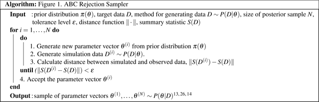
ABC Rejection Sampler Algorithm

The ABC rejection sampler (Figure 1) begins by sampling a parameter vector θ⁽ⁱ⁾ from the prior distribution π(θ). Next, the MSM simulates M trajectories for the n individuals to generate data D⁽ⁱ⁾ given the parameter vector θ⁽ⁱ⁾ - these data are then summarized via the summary statistic S. Third, the distance ||S(D⁽ⁱ⁾)−S(D)|| between the model predictions S(D⁽ⁱ⁾) and calibration target S(D) is calculated, and if this distance is less than ε the proposed parameter vector is accepted. Steps 1–3 are repeated until N sets of parameters have been accepted. The resulting sets of parameter values are an independent sample from the approximate posterior distribution.²⁶

2.2. ABC Markov Chain Monte Carlo algorithm

A variant of the ABC algorithm combines ABC with Markov Chain Monte Carlo (MCMC) algorithms (Figure 2).¹⁶ MCMC algorithms (e.g., Metropolis and Gibbs samplers) sample from an arbitrary probability distribution, and are widely applied in Bayesian inference.²⁷

Figure 2.

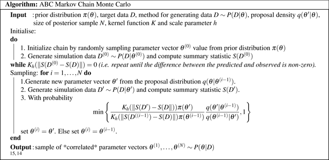
ABC-MCMC Algorithm

The ABC MCMC algorithm is initialized by randomly sampling a proposed parameter vector θ⁽⁰⁾ from the prior distribution π(θ). Second, the MSM generates data D⁽⁰⁾ by simulating individual trajectories of patients given the newly proposed set of parameters θ⁽⁰⁾ and the data are summarized via the summary statistic S. The distance between the predictions and the observed target ||S(D⁽⁰⁾ −S(D)|| is re-scaled using a kernel smoothing function K_h with a scale parameter h > 0, with $K_h(x)=\frac{1}{h}{K}_h\left(\frac{x}{h}\right)$. This kernel function discriminates between predictions that are close to the target and predictions that are further from the target, unlike the use of a tolerance in the ABC rejection sampler algorithm, where a parameter set is always accepted if the distance between the predictions and the target are less than the tolerance. The use of a Gaussian kernel function $K(x)=\frac{1}{\sqrt{2\pi }}{e}^{-\frac{1}{2}{x}^2}$ decreases the time needed for the chain to converge.^28,15 The initialization process stops when the scaled distance is greater than 0 and this scaled distance value is stored.

Following the initialization procedure, the algorithm generates a new vector of parameter values θ⁽ⁱ⁾ from the proposal density q(θ′|θ). The proposal density is a function which determines the next proposed parameter value in the MCMC chain conditional on the current accepted parameter value. Next, the MSM simulates patients to generate data D given the parameter vector θ⁽ⁱ⁾. These data are then summarized via the summary statistic S(D), and the distance between the summarized model predictions and observed data ||S(D⁽ⁱ⁾)–S(D)|| is re-scaled using the kernel smoothing function. The probability of accepting the proposed parameter value is then calculated as:

$$\min \left\{\frac{K_h\left(\Vert S\left(D^{\prime }\right)-S(D\Vert )\right)\pi \left({\theta }^{\prime }\right)}{K_h(\Vert S(D((i-1))-S(D)\Vert )\pi ({\theta }^{(i-1)})}\frac{q\left({\theta }^{\prime }\mid {\theta }^{(i-1)}\right)}{q\left({\theta }^{(i-1)}\mid {\theta }^{\prime }\right)},1\right\}$$ (2)

Smaller values of h decrease the overall acceptance rate of the algorithm, whereas larger values of h increase the acceptance rate. If h is too small, the accuracy of the posterior approximation will improve, but the algorithm will take longer to converge. If h is too large, the accuracy of the posterior approximation decreases, but the algorithm will converge faster.¹⁵ A range of h values can be determined where the acceptance rate is greater than 0 and less than 1. Parameters from this range should be tested to observe the effect on the approximate posterior as well as the effect on the acceptance rate of the algorithm runs. These results can then be used to choose a final value for the scale parameter.

If the newly proposed value is accepted, the chain then moves to the new value θ⁽ⁱ⁾, otherwise it stays at the previous position θ⁽ⁱ⁻¹⁾. The sampling then repeats for N steps.

A common choice for the proposal distribution q(θ′|θ) is to use a random walk, e.g., to add a (multivariate) normal random variable with mean 0 and a chosen standard deviation to the previously accepted parameter value(s). In this case the proposal distribution is symmetric, and therefore the acceptance probability formula reduces to:

$$\min \left\{\frac{K_h\left(\Vert S\left(D^{\prime }\right)-S(D\Vert )\right)P\left({\theta }^{\prime }\right)}{K_h\left(\Vert S\left(D^{((i-1)}\right)-S(D)\Vert \right)P\left({\theta }^{(i-1)}\right)},1\right\}$$ (3)

If the chosen standard deviation is too small, the chain will move too slowly, whereas if the chosen standard deviation is too large, the chain will reject too large a number of proposed parameters.²⁹ Inspecting the plot of parameter values of the chain (the trace plot) can help determine if the choice of scale parameter and proposal function are acceptable. If values are proposed that have a prior probability of 0, they will be rejected because the prior distribution evaluated at the current parameter set in the chain is in the numerator of the Metropolis acceptance formula.

Common issues with MCMC algorithms are that the chain takes time to converge, samples drawn prior to convergence are not from the posterior distribution, and that the resulting sample is not independent, but is autocorrelated due to the sequential nature of the MCMC algorithm. It is common to determine when the chain has converged and to eliminate the first N samples of the algorithm that were drawn prior to convergence. This technique is called burn-in. Autocorrelation is corrected for by the use of thinning, which is the acceptance of only one of every T samples from the posterior.

2.3. Other ABC Algorithms

Computing time is a challenge when implementing Bayesian calibration.¹⁵ Vectorization, which simultaneously moves patients in the model from state to state in a discrete time MSM, can improve efficiency.³⁰ Paralellization reduces the computation time of the ABC rejection sampler, but has a smaller benefit for ABC-MCMC as it can only be applied to a restricted portion of the entire process (e.g., simulating individual trajectories in parallel) due to the sequential nature of the algorithm. Even with these improvements, the ABC rejection sampler and ABC-MCMC algorithms may not be efficient enough to calibrate a large number of model parameters.

Variants of the ABC algorithm have been developed to reduce computation time. One popular ABC algorithm is Sequential Monte Carlo ABC (ABC-SMC).³¹ ABC-SMC improves efficiency by ensuring that a larger proportion of proposed parameters come from a region of high posterior density. This is achieved by creating a sequence of sampling distributions f₀(θ), f₁(θ),... that converge to the posterior distribution.¹⁵ Incremental Mixture Approximate Bayesian Computation (IMABC) is another ABC variant. IMABC begins with a ABC rejection sampler step, and then draws additional samples from a mixture of multivariate distributions centered at points accepted by the ABC rejection sampler. This algorithm was developed for the purpose of calibrating microsimulation models.¹² Both the ABC-SMC and IMABC algorithms can be parallelized.

Software is available to implement the different ABC algorithms in many different programming environments. The R package ”EasyABC” implements the ABC rejection sampler, ABC-MCMC, and ABC-SMC.²⁶ The recent R package ”imabc” implements the IMABC algorithm. Both of these packages are available on CRAN.

2.4. Calibration Diagnostics and Reporting of Results

To assess the results from an ABC calibration procedure, the posterior predictive distribution should be calculated. The posterior predictive distribution is the distribution of model predictions conditioned on the observed data. The output of the ABC algorithms is a set of parameters drawn from the approximate posterior distribution, together with the predictions simulated from the set of parameters. These predictions are a sample from the approximate posterior predictive distribution. The posterior predictive distribution can be visualized and compared to the calibration targets, in a method known as predictive visual checks.³²

The posterior and posterior predictive distributions can also be used to calculate a ”credible interval” - the Bayesian analogue of a confidence interval. A (100)(1−α)% credible interval for a single dimensional posterior distribution is defined as an interval [a,b] in the parameter space such that:

$${\int }_a^{b}P(\theta \mid D)d\theta =1-\alpha$$

There are multiple methods of calculating credible intervals which can produce different results.³³ In our examples, we use the equal tailed interval (ETI) method of calculating credible intervals. For example, the 90% equal tailed credible interval for a given single dimension posterior distribution contains the central portion of the posterior distribution, excluding the values that are less than the 5th percentile and greater than the 95th percentile. No assumption of normality on the posterior distribution is necessary to calculate a credible interval. Credible intervals for the posterior predictive distribution that do not contain the calibration target indicate poor fit.

Final reporting of the calibration procedure should graphically present the prior distribution, approximate posterior distribution, approximate posterior predictive distribution, calibration target, and credible interval. Pairwise plots of accepted parameters can help to identify relationships between calibrated parameters.

3. APPLICATION OF ABC FOR MSM CALIBRATION

3.1. Dementia Microsimulation Model

We illustrate the implementation of ABC calibration using a streamlined version of a published dementia model (R Code: Appendix 1),³⁴ that predicts transitions between the community and nursing home. This streamlined version consists of three states: living in the community, living in a nursing home, and deceased. An individual enters the model as a community-dwelling incident case, and at each cycle (month) can transition to any of the three states. The monthly probability of transitioning from the community to nursing home is derived from a Weibull proportional hazards regression estimated using data from the National Alzheimer’s Coordinating Center Uniform Data Set.³⁴ Another Weibull proportional hazards regression predicts the monthly probability of leaving a nursing home. This model was fit using Medicare data. Each Weibull regression has coefficients for an individual’s age of dementia onset, sex, and race. In this parameterization, the Weibull cumulative hazard function is given by

$$H(t)=\exp (\mathbf{X}\beta )t^a$$ (4)

where a is the shape of the Weibull distribution, X is the covariates and β are the coefficients.

The difference of the cumulative hazard between two months is calculated and transformed into a monthly probability of transitioning to or from the nursing home. Mortality is predicted using age and race stratified published survival estimates for people living with dementia.³⁵

3.2. Example 1: Single Parameter and Single Target

Prior to calibration (see eTable 1 for original model parameters), the streamlined dementia MSM predicts 6.4% of people die in the nursing home. In comparison, a published study reports 48.8% of Medicare beneficiaries living with dementia die in the nursing home.³⁶ We applied ABC to calibrate the dementia MSM predicted place of death towards the proportion reported in the literature. We calibrated the intercept of the Weibull regression β₀ predicting transition to a nursing home, which can be thought as an adjustment of the baseline risk of transition to a nursing home. We fixed the coefficients of age, sex, race, and shape to their point estimates from the model prior to calibration.

We do not have information to inform the prior distribution of the Weibull intercept, and have therefore opted to use a diffuse prior. To inform the choice of a diffuse prior distribution of the Weibull intercept, we conducted an empirical calibration using a search of a Unif(−20,0) distribution, and ultimately a prior distribution of Unif(−10,−5) was selected.

Using the age, sex, and race distribution observed in the target data, we sampled a cohort of n = 100 individuals and the cohort was repeatedly simulated M = 10 times for a total of 1,000 microsimulations per parameter tested. Our summary statistic S summarizes the microsimulation results by calculating the proportion of simulated patients who die in a nursing home. We chose values for n,M that were large enough to reduce variation and could be conducted in a reasonable amount of time. This cohort is saved and new trajectories for the cohort are simulated for each set of parameter values tested.

We aimed to complete analyses within 3 hours, which allowed us to obtain N = 100 samples from the approximate posterior distribution. We set the maximum computing time to three hours so that it is easy to recreate our example. Additional computation would be needed in a more complex analysis. We compared the mean and standard deviation of the first 25, 50, 75, and 100 parameters accepted by the ABC algorithms, to observe how the distribution changes as new samples are drawn (eFigures 1 and 2). The mean and standard deviation of the approximate posterior distribution did not substantially change when the size of the sample increased from 75 to 100.

We used root mean squared error (RMSE)

$$\text{RMSE}=\sqrt{\frac{{\sum }_{i=1}^N{\left(y_i-x_i\right)}^2}{N}}$$ (5)

where y = (y₁,...,y_n) is the vector of predicted summary statistics and x = (x₁,...,x_n) is the vector of observed summary statistics, to calculate the distance between the model predictions and the calibration target. In this 1-dimensional case, RMSE is equivalent to absolute value, since the formula reduces to $\sqrt{{\left(y_1-x_1\right)}^2}=\left|y_1-x_1\right|$.

For the ABC rejection sampler (R Code: Appendix 2), we evaluated a range of values of ε (ε = 0.5%,1%,2.5%,5%) to examine how the approximation changed with varying tolerances. We tested parameter values until 100 (i.e., our predefined target sample size approximate posterior distribution) were accepted for each of the tested tolerance values.

For the ABC-MCMC algorithm (R Code: Appendix 3), we used a Gaussian kernel and random-walk Metropolis algorithm. The Gaussian kernel has been empirically observed to decrease the convergence time of the algorithm, and the random-walk Metropolis algorithm was chosen to simplify the calculation of the Metropolis acceptance probability.¹⁴ We tested different values of h (h = 0.01,0.025,0.05,0.1) to examine how the approximation changed as the scale parameter was varied. These values were chosen because the algorithm had too high of a rejection rate for values of h < 0.01 and too low of a rejection rate for values of h > 0.1. We ran the chain with a length of 2,500, a burn in period of 500 and a thinning of 20, producing a sample of exactly 100 values. The burn-in period was chosen based on visual inspection of the trace plot of accepted parameter values to determine convergence (eFigure 3). We tested different possible thinning values and observed how the autocorrelation plot of the posterior sample was affected (eFigure 4).

Both the ABC rejection Sampler (Figure 3) and the ABC MCMC algorithm (Figure 4) identified similar posterior distributions for the calibration parameter. The mean predicted value and 90% credible interval of the posterior predictive distribution obtained by the ABC rejection sampler (ε = 0.5%, 0.488 90% CI: [0.484, 0.492]) and ABC MCMC (h = 0.01, 0.489 90% CI: [0.469, 0.505]) both overlapped with the calibration target (0.488) indicating good fit (Figures 3B and 4B). The posterior distribution of the ABC rejection sampler and ABC MCMC algorithm narrowed as ε and scale parameter h decreased and the predictive means remained close to the calibration target (eTable 2).

Figure 3.

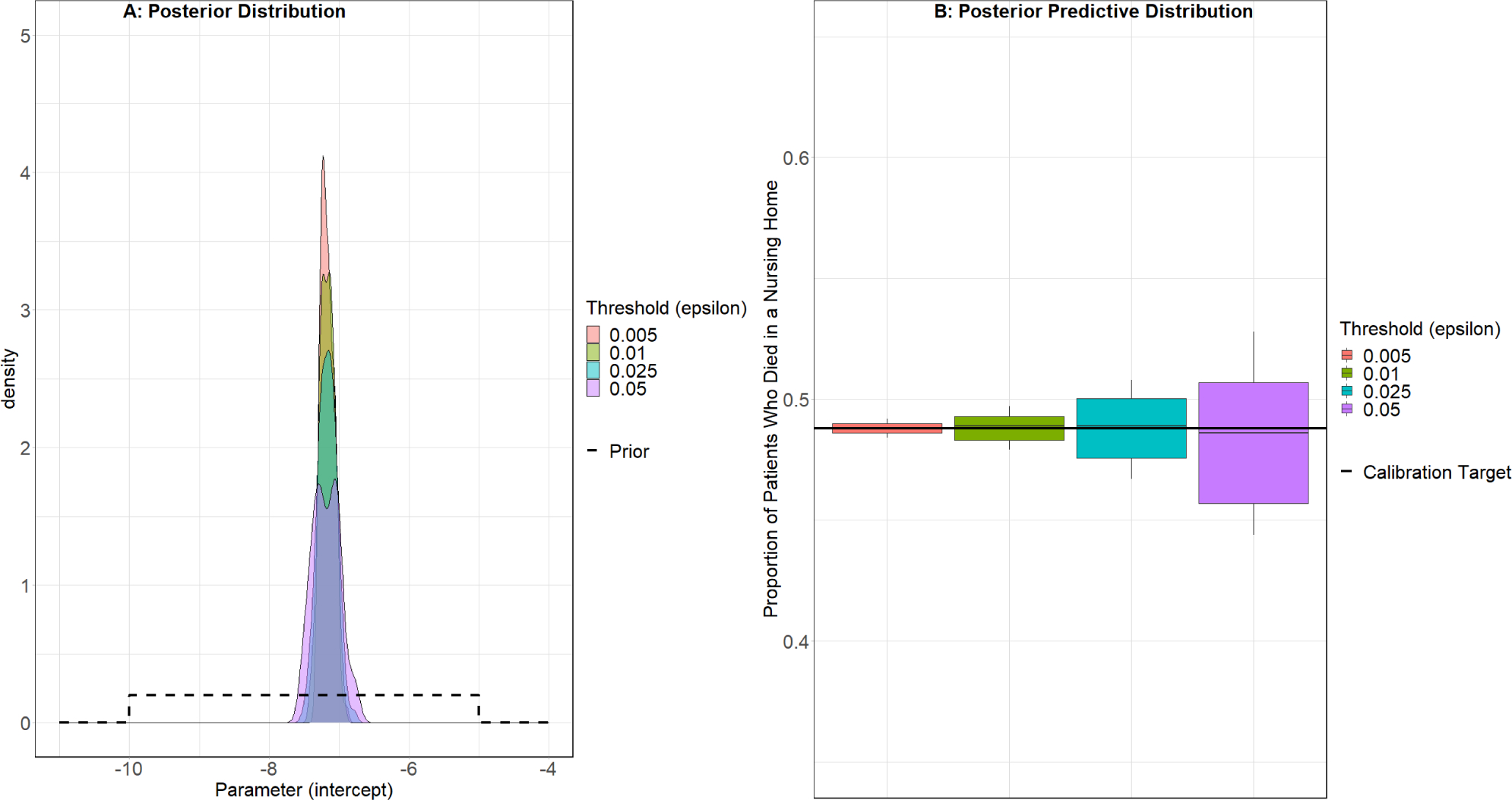
ABC Rejection Sampler Results: Place of Death Calibration Target *

* Boxplot whiskers represent the 90% credible interval for the distribution, instead of the common usage of 1.5 times the interquartile range.

Figure 4.

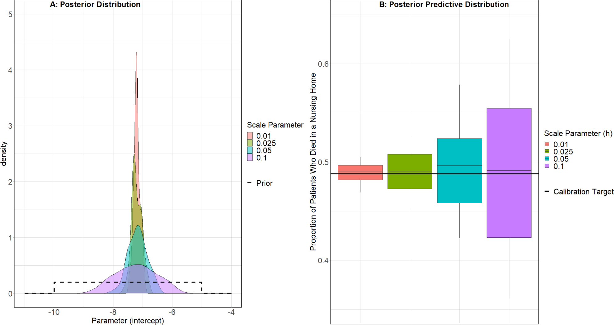
ABC MCMC Results: Place of Death Calibration Target *

* Boxplot whiskers represent the 90% credible interval for the distribution, instead of the common usage of 1.5 times the interquartile range.

3.3. Example 2: Multiple Parameters and Multiple Targets

Prior to calibration, the dementia MSM predicted time in the nursing home deviates from values observed in Medicare data (Table 2; eTable 1 for model parameters). As an example of a multidimensional calibration, we applied ABC to calibrate the dementia MSM towards the average time a person with dementia spends in a nursing home, stratified by sex, race, and life expectancy (3–7 years following diagnosis) as reported in Medicare data (see Target column in Table 2).

Table 2.

Multidimensional Calibration Example Results

Race	Sex	Months to Death Post Diagnosis	Target	Original Model Predictions (Mean)	ABC Rejection (ε = 2) Calibrated Model Predictions (Mean, 90% Credible Interval)	ABC MCMC (h = 0.5) Calibrated Model Predictions (Mean, 90% Credible Interval)
White	Men
		25–36 Months	3.90	0.48	2.69 [1.68, 4.01]	2.92 [2.08, 3.86]
		37–48 Months	5.43	1.15	4.88 [3.34, 6.88]	5.14 [3.86, 6.52]
		49–60 Months	6.74	1.75	7.33 [5.13, 9.75]	7.48 [5.77, 9.11]
		61–72 Months	8.47	2.65	9.75 [6.85, 12.94]	9.71 [7.59, 11.85]
	Women
		25–36 Months	5.04	0.52	3.32 [2.15, 4.71]	3.60 [2.62, 4.72]
		37–48 Months	7.24	1.11	5.85 [4.24, 7.90]	6.11 [4.65, 7.54]
		49–60 Months	9.81	1.93	8.70 [6.39, 11.22]	8.80 [6.87, 10.66]
		61–72 Months	12.64	2.96	12.17 [8.96, 15.55]	12.01 [9.59, 14.51]
Black	Men
		25–36 Months	4.79	0.24	2.78 [1.72, 4.22]	3.07 [2.08, 4.08]
		37–48 Months	6.16	0.54	4.71 [3.17, 6.76]	5.03 [3.67, 6.40]
		49–60 Months	8.61	0.83	7.28 [5.06, 9.82]	7.56 [5.65, 9.46]
		61–72 Months	10.29	1.36	10.56 [7.38, 13.86]	10.65 [8.10, 13.19]
	Women
		25–36 Months	4.34	0.28	3.58 [2.36, 5.06]	3.87 [2.81, 4.92]
		37–48 Months	6.85	0.51	6.02 [4.31, 8.06]	6.31 [4.91, 7.80]
		49–60 Months	9.04	1.03	8.90 [6.51, 11.46]	9.03 [7.16, 11.03]
		61–72 Months	11.31	1.46	12.59 [9.20, 16.01]	12.45 [10.19, 15.01]
Other	Men
		25–36 Months	3.42	0.24	2.05 [1.15, 3.36]	2.34 [1.54, 3.20]
		37–48 Months	5.20	0.62	3.48 [2.14, 5.28]	3.87 [2.70, 5.08]
		49–60 Months	6.59	1.15	5.54 [3.51, 8.01]	5.88 [4.18, 7.57]
		61–72 Months	7.14	1.46	7.87 [4.86, 11.16]	8.14 [5.86, 10.46]
	Women
		25–36 Months	3.40	0.39	2.54 [1.51, 3.86]	2.86 [1.95, 3.84]
		37–48 Months	4.83	0.62	4.43 [2.85, 6.33]	4.80 [3.30, 6.27]
		49–60 Months	6.74	1.11	6.48 [4.28, 9.09]	6.78 [4.81, 8.63]
		61–72 Months	8.64	1.61	8.79 [5.73, 12.14]	9.00 [6.42, 11.52]

We calibrated the sex, race, intercept, and shape parameters of the Weibull regression predicting transition to a nursing home. We conducted an empirical calibration using Latin hypercube sampling to identify a space of plausible values for the model parameters to inform their respective prior distributions. The intercept was highly correlated with the shape which causes nonidentifiability (where multiple parameter sets solve the calibration problem) (eFigure 5). To eliminate this issue, we propose new intercept values as a linear function of the shape. Identifying relationships between parameters can help reduce the total number of parameters that need to be calibrated. Parameter values that produced a prediction with an RMSE within 5 of the calibration target were accepted in our empirical calibration (eTable 3).

For each of the 24 stratifications (Table 2) we sampled 100 individuals, for a total of n = 2,400 individuals. This cohort was then simulated M = 5 times for a total of n_s = 12,000 microsimulations. As before, we found that this value was large enough to reduce variation, and could be conducted in a reasonable amount of time. The microsimulations are summarized by calculating the average time in a nursing home within each stratification. We aimed to complete analyses within 24 hours which allowed us to obtain a sample of at least 1,000 values from the approximate posterior distribution. We compared the mean and standard deviation of the first 250, 500, 750, and 1,000 parameters accepted by the ABC algorithm. The approximate posterior distribution did not substantially change the mean and standard deviation when the size of the sample was increased from 750 to 1,000. We used the RMSE distance function between the model predicted and target observed time in the nursing home for both the ABC rejection sampler and ABC MCMC.

For the ABC rejection sampler (R Code: Appendix 4), we selected a tolerance of ε = 2, and tested values until the predictions of at least 1,000 sets of parameters met the acceptance criteria.

In implementing the ABC MCMC algorithm (R Code: Appendix 5), we used a Gaussian kernel, random-walk Metropolis algorithm, and a scale h parameter of 0.5. To obtain 1,000 samples from the approximate posterior distribution, we ran the chain with a length of 25,000, a burn in period of 5,000 and a thinning of 20. The choice of burn-in and thinning values were determined with the same method as the previous example.

The ABC rejection sampler and ABC MCMC algorithm identified similar posterior distributions for each of the parameters (eFigures 6, 7). The predictions from the ABC rejection algorithm were less accurate with our chosen threshold than those generated by the ABC MCMC algorithm. While the mean and 90% credible interval of the posterior predictive distribution obtained from the ABC rejection sampler and MCMC algorithm overlapped with most of the target data (eFigures 8, 9), the credible intervals for the predictions obtained from the rejection sampler are wider than those obtained from the MCMC algorithm.

Neither algorithm fit perfectly to the calibration targets, as can be seen in (eFigures 8,9), though there was an improvement from the predictions of the model prior to calibration (eTable1, Table 2). The accuracy of the predictions could potentially be improved by reducing the value of the threshold/scale parameter, which will necessarily lead to an increase in computation time to achieve the same sized sample. If a model fails to achieve a desired similarity to the calibration target, adjustment of the model structure may be necessary.

4. DISCUSSION

We provide a tutorial for implementing an ABC rejection sampler and ABC-MCMC for calibrating MSMs. These algorithms are relatively easy to implement, can be applied to any simulation model, account for parameter uncertainty, and do not require calculation of the likelihood function. However, ABC algorithms are time consuming, the posteriors are an approximation, and there is limited guidance on how to choose algorithm inputs (e.g. the distance function, threshold). Our tutorial provides a basic conceptual framework to understand calibration and focuses on the application of approximate Bayesian calibration to MSMs. Detailed descriptions of calibration and approximate Bayesian methods can be found elsewhere.^13,3,4,15

In our analyses, computation time was considerably greater in the example with multiple targets than the example with a single target. We also saw that the introduction of multiple calibration targets makes it more difficult to fit to each target. The ABC rejection sampler is easier to implement than other ABC algorithms, but it is also less efficient. The ABC-MCMC algorithm is more likely to propose parameters that will be accepted because every value accepted by the chain after it has converged to the stationary distribution is a random draw from the target posterior distribution. However, ABC-MCMC has other challenges including: autocorrelation of the sample, the algorithm cannot be parallelized, and convergence of the chain can be difficult to ascertain. Other MCMC methods can potentially be integrated into ABC-MCMC to help mitigate these concerns (e.g., burn-in).¹⁵ In our first example, both algorithms were easily able to fit to one calibration target when calibrating one parameter. In the example with multiple calibration targets, the ABC-MCMC algorithm predictions were closer to the target than the ABC rejection sampler, when both algorithms were given the same prior distributions and amount of computing time. By reducing the tolerance of the ABC rejection sampler algorithm, we could match the results of the ABC-MCMC algorithm, but this requires an increase in computing time.

We did not explore the effect of changing the choice of summary statistic or distance measure on the approximation of the posterior distribution. Finally, our example calibration fits only to outcomes on the same scale. A possible method for calibrating to multiple targets with different types of outcomes (i.e. discrete or continuous or across multiple scales) is to use a weighted distance function (such as weighted RMSE), with weights assigned to the different types of targets.

In conclusion, the ABC rejection sampler and ABC-MCMC are two powerful approaches to implement calibration procedures in the context of microsimulation modelling. Both methods successfully find a posterior distribution that produces outcomes similar to the calibration target. The implementation of calibration ultimately supports the goal of modeling which is to improve decision making by using models that can accurately replicate observed data.

Table 1.

Considerations for Approximate Bayesian Computation Algorithms

	Description	Recommendation	Notation
Step 1: Establish Calibration Problem
Define Calibration Problem and Identify Calibration Target	Identify calibration targets, model predicted outcome(s) that should be similar to outcome(s) from an external source. Generally, these consists of summary measures such as means or proportions.	Target outcomes should be meaningful for decision makers or model end users.	D: target data S(D): summary of target data $\widehat{D}$: model prediction of target data
Identify Model Parameters to Calibrate	Identify model parameters to calibrate.	Parameters should be selected based on whether or not they affect the calibration target outcome, and whether or not a good estimate for the parameter in question exists.	θ: Set of parameters being calibrated.
Determine Prior Distribution of Parameters to be Calibrated	Describes what is known about the distribution of the parameters to be calibrated. The calibration procedure samples from this distribution.	If possible, incorporate known information about the distribution of a target parameter. Otherwise, a uniform prior or other uninformative prior can be chosen. Posterior predictive checks can eliminate unlikely parameter values from consideration.	π(θ): prior distribution for model parameters to be calibrated
Determine Number of Simulations	Determine how many patients are simulated and how many times at each step of the calibration algorithm. The simulation process can be computationally taxing, and there is a trade-off between computation time and variance of the distribution of predicted outcome P(D|θ).	Use a sufficiently large number of simulations to ensure reasonable computation time and small enough variance. Or, conduct simulations with varying levels of n and k to determine optimal combination.	n: number of patients k: number of times the n patients are simulated
Determine Sample Size of the Posterior Distribution	The size of the sample drawn from the posterior distribution P(θ|D) in the calibration procedure.	Limited guidance in the literature in the application of approximate Bayesian calibration, but in practice the sample size should be sufficiently large that the researcher can obtain summary measures from the posterior distribution with minimal error. Size of the sample may also be limited by the computational budget of the researcher.	N: size of the sample drawn from the posterior distribution P(θ|D): posterior distribution of new model parameter conditioned on the calibration target data.
Distance Measure	Calculates how far the model predicted outcomes S($S(\widehat{D})$ are from the target outcomes S(D) given a sampled parameter set ($\widehat{\theta }$).	A measure appropriate for the data type and how the predictions are expected to fit the observed data. There many possible distance measures, including Euclidean distance, (root) mean squared error, Mahalanobis distance.	||·||
Step 2: Implement ABC Approach
ABC Rejection Sampler Considerations
Threshold	Determines if a parameter value is likely to be sampled from the posterior distribution of target outcome P(θ|D)	When calibration is only used for prediction than ε ≥ 0 should be as close to 0 as feasible. When calibration is used for prediction and uncertainty analysis, then an ε ≥ 0 should be chosen that replicates the uncertainty observed in the target outcome.	ε
MCMC Rejection Sampler Considerations
Kernel function	Is a weighted function of the difference between model predicted $\widehat{D}$ and target data D. The function gives greater importance to predicted $\widehat{D}$ values that are closer to D. Kernel smoothing functions are often applied in statistics.	A Gaussian kernel has been recommended over kernel functions with compact support, since they have been shown in an empirical study to reduce the convergence time of the algorithm.28	K
Scale parameter	Scales the curve of the kernel function and helps determine the acceptance probability. Larger scale parameter values cause a higher proportion of tested values being accepted, while small scale parameter values cause a smaller proportion of tested values to be accepted.	Empirically test different values until a reasonable proportion of tested parameter values are accepted.	h
Proposal density	Determines the next proposed parameter value in the MCMC chain conditional on the current sampled parameter value.	Random normal variable (mean = 0 and SD = scaled to the parameters magnitude) added to the previous value.	q(θ′|θ)
Step 3: Final Reporting Considerations
Compare Posterior Predictive Distribution With Calibration Target	Visually compare the posterior predictive distribution with the calibration targets. Targets lying outside of the distribution indicate poor fit.	Use boxplot to visualize the posterior predictive distribution and include calibration targets in the plot.
Other Considerations	Comprehensively report all elements of the calibration procedure.	Graphically present approximate posterior and posterior predictive distributions. Include choices of distance function, number of simulations, sample size of posterior distribution, and other necessary algorithm inputs.

REFERENCES

- 1.Chrysanthopoulou S MILC: A microsimulation model of the natural history of lung cancer. Int J Microsimulation. 2017;10(3):5–26. [Google Scholar]
- 2.Rutter CM, Zaslavsky AM, Feuer EJ. Dynamic Microsimulation Models for Health Outcomes. Med Decis Making. 2011;31(1):10–18. [DOI] [PMC free article] [PubMed] [Google Scholar]
- 3.Taylor DCA, Pawar V, Kruzikas D, Gilmore KE, Pandya A, Iskandar R, Weinstein MC. Methods of model calibration: observations from a mathematical model of cervical cancer. Pharmacoeconomics. 2010;28(11):995–1000. [DOI] [PubMed] [Google Scholar]
- 4.Kennedy MC, O’Hagan A. Bayesian calibration of computer models. J R Statist Soc B. 2001;63(3):425–464. [Google Scholar]
- 5.Doubilet P, Begg CB, Weinstein MC, Braun P, McNeil BJ. Probabilistic sensitivity analysis using Monte Carlo simulation: a practical approach. Med Decis Making. 1985;5(2):157–177 [DOI] [PubMed] [Google Scholar]
- 6.Rutter CM, Miglioretti DL, Savarino JE. Bayesian Calibration of Microsimulation Models. J Am Stat Assoc. 2009;104(488):1338–1350. [DOI] [PMC free article] [PubMed] [Google Scholar]
- 7.Claxton KP, Sculpher MJ. Using value of information analysis to prioritise health research. Pharmacoeconomics. 2006;24(11):1055–1068. [DOI] [PubMed] [Google Scholar]
- 8.Wong RKW, Storlie CB, Lee TCM. A frequentist approach to computer model calibration. J R Statist Soc B. 2017;79(Pt2):635–648. [Google Scholar]
- 9.Marjoram P, Hamblin S, Foley B. Simulation-based Bayesian Analysis of Complex Data. Summer Comput Simul Conf (2015). 2015;47(10):176–183. [PMC free article] [PubMed] [Google Scholar]
- 10.Beaumont MA, Zhang W, Balding DJ. Approximate Bayesian Computation in Population Genetics. Genetics. 2002;162(4):2025–2035. [DOI] [PMC free article] [PubMed] [Google Scholar]
- 11.Turner BM, Zandt TV. A tutorial on approximate Bayesian computation. J Math Psychol. 2012;56(2):69–85. [Google Scholar]
- 12.Rutter CM, Ozik J, DeYoreo M, et al. Microsimulation model calibration using incremental mixture approximate Bayesian computation. The Annals of Applied Statistics 2019; 13. DOI: 10.1214/19-aoas1279. [DOI] [PMC free article] [PubMed] [Google Scholar]
- 13.Menzies NA, Soeteman DI, Pandya A, Kim JJ. Bayesian methods for calibrating health policy models: a tutorial. PharmacoEconomics. 2017;35(6):613–624. [DOI] [PMC free article] [PubMed] [Google Scholar]
- 14.Pritchard JK, Seielstad MT, Perez-Lezaun A, Feldman MW. Population growth of human Y chromosomes: a study of Y chromosome microsatellites. Mol Biol Evol. 1999. Dec;16(12):1791–1798. [DOI] [PubMed] [Google Scholar]
- 15.Sisson SA, Fan Y, Beaumont M. Handbook of approximate Bayesian computation. CRC Press, Taylor Francis Group;2019. [Google Scholar]
- 16.Marjoram P, Molitor J, Plagnol V, Taváre S. Markov chain Monte Carlo without likelihoods. Proc Natl Acad Sci U S A. 2003;100(26):15324–15328. [DOI] [PMC free article] [PubMed] [Google Scholar]
- 17.Aronica G, Hankin B, Beven K. Uncertainty and equifinality in calibrating distributed roughness coefficients in a flood propagation model with limited data. Adv Water Resour. 1998;22(4):349–365. [Google Scholar]
- 18.Vanni T, Karnon J, Madan J, White RG, Edmunds W, Foss AM, Legood R. Calibrating models in economic evaluation: a seven-step approach. Pharmacoeconomics. 2011;29(1):35–49. [DOI] [PubMed] [Google Scholar]
- 19.Ramsey SD, McIntosh M, Etzioni R, Urban N. Simulation modeling of outcomes and cost effectiveness. Hematol Oncol Clin North Am. 2000;14(4):925–938. [DOI] [PubMed] [Google Scholar]
- 20.Salomon JA, Weinstein MC, Hammitt JK, Goldie SJ. Empirically calibrated model of hepatitis C virus infection in the United States. Am J Epidemiol. 2002. Oct 15;156(8):761–773. [DOI] [PubMed] [Google Scholar]
- 21.Chrysanthopoulou SA, Rutter CM, Gatsonis CA. Bayesian versus empirical calibration of Microsimulation Models: A comparative analysis. Medical Decision Making; 41: 714–726. [DOI] [PMC free article] [PubMed] [Google Scholar]
- 22.Chia YL, Salzman P, Plevritis SK, Glynn PW. Simulation-based parameter estimation for complex models: a breast cancer natural history modelling illustration. Stat Methods Med Res. 2004. Dec;13(6):507–524. [DOI] [PubMed] [Google Scholar]
- 23.Calvello M, Finno RJ. Selecting parameters to optimize in model calibration by inverse analysis. Comput Geotech. 2004;31(5):410–424. [Google Scholar]
- 24.van de Schoot R, Depaoli S, King R, et al. Bayesian statistics and modelling. Nature Reviews Methods Primers 2021; 1. DOI: 10.1038/s43586-020-00001-2. [DOI] [Google Scholar]
- 25.Sunnaker M, Busetto AG, Numminen E, Corander J, Foll M, Dessimoz C. Approximate Bayesian Computation. PLoS Comput Biol. 2013;9(1):e1002803. [DOI] [PMC free article] [PubMed] [Google Scholar]
- 26.Jabot F, Faure T, Dumoulin N. Easy ABC: performing efficient approximate Bayesian computation sampling schemes using R. Methods Ecol. Evol. 2013;4(7):684–687. [Google Scholar]
- 27.Robert C, Casella G. A Short History of Markov Chain Monte Carlo: Subjective Recollections from Incomplete Data. Statistical Science. 2011;26(1):102–115. [Google Scholar]
- 28.Sisson SA, Fan Y. Likelihood-free Markov chain Monte Carlo. 2010. In MCMC handbook, Brooks SP, Gelman A, Jones G and Meng X-L (eds), Chapman ‘l&’ Hall. [Google Scholar]
- 29.Sherlock C, Fearnhead P, Roberts GO. The Random Walk Metropolis: Linking Theory and Practice Through a Case Study. Statist. Sci. 2010;25(2):172–190. [Google Scholar]
- 30.Krijkamp EM, Alarid-Escudero F, Enns EA, Jalal HJ, Hunink MGM, Pechlivanoglou P. Microsimulation Modeling for Health Decision Sciences Using R: A Tutorial. Med Decis Making. 2018;38(3):400–422. [DOI] [PMC free article] [PubMed] [Google Scholar]
- 31.Sisson SA, Fan Y, Tanaka MM. Sequential Monte Carlo without likelihoods. Proceedings of the National Academy of Sciences. 2007;104(6):1760–5. [DOI] [PMC free article] [PubMed] [Google Scholar]
- 32.Lemaire L, Jay F, Lee IH, Csilĺery K, Blum MGB. Goodness-of-fit statistics for approximate Bayesian computation. ArXiv:1601.04096; 2016. [Google Scholar]
- 33.Makowski D, Ben-Shachar MS, Ludecke D. bayestestR: Describing Effects and their Uncertainty, Existence and Significance within the Bayesian Framework. J Open Source Softw. 2019;4(40):1541. [Google Scholar]
- 34.Jutkowitz E, Kuntz KM, Dowd B, Gaugler JE, Maclehose RF, Kane RL. Effects of cognition, function, and behavioral and psychological symptoms on out-of-pocket medical and nursing home expenditures and time spent caregiving for persons with dementia. Alzheimers Dement. 2017;13(7):801–809. [DOI] [PMC free article] [PubMed] [Google Scholar]
- 35.Mayeda ER, Glymour MM, Quesenberry CP, Johnson JK, Perez-Stable EJ, Whitmer RA. Survival after dementia diagnosis in five racial/ethnic groups. Alzheimers Dement. 2017;13(7):761–769. [DOI] [PMC free article] [PubMed] [Google Scholar]
- 36.Teno JM, Gozalo PL, Bynum JPW, Leland NE, Miller SC, Morden NE, Scupp T, Goodman DC, Mor V. Change in End-of-Life Care for Medicare Beneficiaries Site of Death, Place of Care, and Health Care Transitions in 2000, 2005, and 2009. JAMA. 2013;309(5):470–477. [DOI] [PMC free article] [PubMed] [Google Scholar]
Associated Data
This section collects any data citations, data availability statements, or supplementary materials included in this article.