TITE-BOIN12: A Bayesian Phase I/II Trial Design to Find the Optimal Biological Dose with Late-onset Toxicity and Efficacy

Summary

In the era of immunotherapies and targeted therapies, the focus of early phase clinical trials has shifted from finding the maximum tolerated dose to identifying the optimal biological dose (OBD), which maximizes the toxicity-efficacy trade-off. One major impediment to using adaptive designs to find OBD is that efficacy or/and toxicity are often late-onset, hampering the designs’ real-time decision rules for treating new patients. To address this issue, we propose the model-assisted TITE-BOIN12 design to find OBD with late-onset toxicity and efficacy. As an extension of the BOIN12 design, the TITE-BOIN12 design also uses utility to quantify the toxicity-efficacy trade-off. We consider two approaches, Bayesian data augmentation and an approximated likelihood method, to enable real-time decision making when some patients’ toxicity and efficacy outcomes are pending. Extensive simulations show that, compared to some existing designs, TITE-BOIN12 significantly shortens the trial duration while having comparable or higher accuracy to identify OBD and a lower risk of overdosing patients. To facilitate the use of the TITE-BOIN12 design, we develop a user-friendly software freely available at www.trialdesign.org.

1 |. INTRODUCTION

In the era of targeted therapies and immunotherapies, the focus of early phase trials has shifted from finding maximum tolerated dose (MTD) to identifying optimal biological dose (OBD), defined as the dose that optimizes the risk-benefit trade-off of the treatment. For these novel agents, efficacy may not monotonically increase with the dose,^1,2 and thus MTD may not be the optimal dose for treating patients. Numerous phase I/II dose-finding designs have been proposed that take into consideration the trade-off between toxicity and efficacy. Thall and Russell developed a Bayesian phase I/II design that characterizes patient outcomes using a trinary variable that accounts for both toxicity and efficacy.³ Braun generalized the continual reassessment method (CRM⁴) to accommodate toxicity and efficacy simultaneously.⁵ Thall and Cook proposed the EffTox design, based on the trade-off between toxicity and efficacy.⁶ Yin et al. proposed to use the odds ratio of toxicity and efficacy as a measure of desirability.⁷ Liu and Johnson proposed a robust Bayesian phase I/II design based on a flexible Bayesian dynamic model.⁸ Guo and Yuan proposed a personalized Bayesian phase I/II design that accounts for patient characteristics and biomarker information.⁹ Zang and Lee proposed several adaptive phase I/II trial designs to find the OBD.¹⁰ A robust two-stage design has also been developed to identify OBD.¹¹ Liu et al. proposed a Bayesian phase I/II trial design for immunotherapy that considers the immune response, toxicity, and efficacy.¹² Yuan et al. provided a comprehensive review on model-based phase I/II designs.¹³ Most of the aforementioned designs require complicated model fitting and are complex to implement in practice. In addition, they require that toxicity and efficacy are observed quickly enough to apply the decision rules of the designs.

To simplify the implementation of phase I/II trials, several model-assisted designs have been proposed, but still under the assumption that toxicity and efficacy are quickly observable. Lin and Yin proposed a simple toxicity and efficacy interval (STEIN) design to find a safe dose with the highest efficacy.¹⁴ Takeda et al. developed the BOIN-ET design to extend the Bayesian optimal interval (BOIN) design to phase I/II trials.¹⁵ Zhou et al. proposed the two-stage U-BOIN design, in which the trade-off between efficacy and toxicity is measured by utility elicited from clinicians.¹⁶ Recently, Lin et al. proposed the utility-based Bayesian optimal interval phase I/II (BOIN12) design to find OBD for immunotherapies and targeted therapies.¹⁷ One attractive feature of BOIN12 is its simplicity. To conduct the trial, no complicated model fitting is needed, and clinicians can simply look up the decision table to determine the dose for treating the next cohort of patients. Moreover, BOIN12 has desirable operating characteristics comparable to or better than some existing, more complicated model-based designs (e.g., EffTox). Several trials based on BOIN12 are under development at MD Anderson Cancer Center.

One practical issue we encountered when applying BOIN12 was that of possible late-onset efficacy and toxicity. As a motivating example, consider a phase I/II renal cell carcinoma trial. The objective is to determine the OBD of a novel targeted agent, combined with nivolumab at a fixed dose of 3 mg/kg daily for 2 weeks, in patients with metastatic renal cell carcinoma. Toxicity is defined as a grade 3 or 4 liver, lung, gastrointestinal or endocrine toxicity, or myelosuppression, within 45 days from the start of therapyaccording to Common Terminology Criteria for Adverse Events (CTCAE) version 5. Efficacy is defined as achieving complete response or partial response within 60 days. Patients will be treated in cohorts of three with a maximum sample size of 36. The expected accrual rate is three patients per month. The challenge of designing this trial is that, on average, six new patients will be enrolled by the time the previous cohort of patients complete their efficacy evaluation. The question is: how do we treat these new patients in a timely fashion?

To address this issue, we proposed the time-to-event BOIN12 (TITE-BOIN12) design, which allows for real-time decision making to choose the optimal dose based on available data for new patients when some previous patients’ toxicity and efficacy outcomes are still pending. We consider two approaches to handle the pending outcomes caused by late-onset toxicity and efficacy: Bayesian data augmentation (BDA)¹⁸ and the approximate likelihood approach.¹⁹ Both approaches leverage the follow-up time of pending patients’ outcomes to facilitate real-time decision making. Extensive numerical studies and sensitivity analyses show that TITE-BOIN12 has robust performance across various configurations of trial settings, and it possesses desirable accuracy to identify OBD while greatly shortening trial duration.

The rest of the text is organized as follows. Section 2 briefly reviews the BOIN12 design, and then extends it to TITE-BOIN12 using BDA and the approximated likelihood approach. Section 3 demonstrates the operating characteristics of TITE-BOIN12 through extensive numerical studies. Section 4 evaluates the sensitivity of TITE-BOIN12. Section 5 provides an overview of the web-based software to implement TITE-BOIN12. Section 6 gives a brief summary and discussion.

2 |. METHOD

2.1 |. BOIN12 design

Consider a binary toxicity endpoint Y_T and a binary efficacy endpoint Y_E, with Y_T = 1 indicating dose limiting toxicity (DLT) and Y_E = 1 indicating response. The joint distribution of (Y_T, Y_E) can be equivalently represented by a single variable Y following a multinomial distribution with four categories: Y = {Y₀₁, Y₀₀, Y₁₁, Y₁₀} = {(Y_T, Y_E) = (0, 1), (Y_T, Y_E) = (0, 0), (Y_T, Y_E) = (1, 1), (Y_T, Y_E) = (1, 0)}, with Y_ab = 1, if (Y_T, Y_E) = (a, b), a, b ∈ {0, 1}, 0 otherwise. Define p_ab = Pr(Y_ab = 1) and p = (p₀₁, p₀₀, p₁₁, p₁₀). It follows that the marginal toxicity and efficacy probabilities are π_T = p₁₁ + p₁₀ and π_E = p₀₁ + p₁₁, respectively. See Lin et al.¹⁷ for the more general case that Y_T and Y_E are categorical variables with more than two levels.

BOIN12 uses utility to quantify the toxicity-efficacy trade-off, which is considered in other phase I/II designs.^{9,12,13,20,21} In this approach, as shown in Table 1, we elicit utility for each of the four possible outcomes (i.e., the four categories of Y), denoted as Ψ = (Ψ₀₁, Ψ₀₀, Ψ₁₁, Ψ₁₀), with a higher value representing a more desirable outcome. This can be done as follows: assign the most desirable outcome Y₀₁ (no toxicity, efficacy) a score of Ψ₀₁ = 100, and the least desirable outcome Y₁₀ (toxicity, no efficacy) a score of Ψ₁₀ =0, and then ask clinicians to use them as references to specify scores for the other two outcomes. The utility is shown to be highly flexible and scalable in previous studies.^16,17 It contains marginal (toxicity and efficacy) probabilities based trade-off, i.e., π_E − ωπ_T, where ω is a weight, as a special case. In addition, it is directly applicable to categorical Y_T and Y_E with more than two levels. Table 1 provides an example of the utility approach for a trinary toxicity endpoint (minor/moderate/severe) and a trinary efficacy endpoint (progressive disease (PD)/stable disease (SD)/partial response or complete response (PR/CR)).

TABLE 1.

Examples of utility.

(a) Example 1
	YE = 1	YE = 0
YT = 0	100	40
YT = 1	60	0
(b) Example 2
	YE = 1	YE = 0
YT = 0	100	40
YT = 1	75	0
(b) Example 3
	YE = PR/CR	YE = SD	YT = PD
YT = minor	100	60	35
YT = moderate	65	30	25
YT = severe	30	15	0

PD: progressive disease, SD: stable disease, PR: partial response, CR: complete response.

Given Ψ, the expected utility of a dose, with outcome probabilities p, is given by

$$u=\sum _{a=0}^1\sum _{b=0}^1{\psi }_{ab}{p}_{ab}.$$ (1)

A higher value of u indicates a higher desirability of a dose in the risk-benefit trade-off. The dose with the highest desirability is the OBD. One innovation of BOIN12 is that, rather than modeling the outcome Y, it directly models the dose utility using a quasi-beta-binomial model. This greatly simplifies the estimation of the desirability of the doses, as well as decision making. Specifically, define the standardized utility u* = u/100 ∈ [0, 1], BOIN12 models u* using a binomial distribution with the “quasi-binomial” data D = (x, N):

$$x=\frac{1}{100}\sum _{a=0}^1\sum _{b=0}^1{\psi }_{ab}{n}_{ab},$$ (2)

which can be interpreted as the number of “events” observed from N patients treated at a dose, $0\le x\le N={\sum }_{a=0}^1{\sum }_{b=0}^1{n}_{ab}$, where n_ab is the number of patients with Y_T = a and Y_E = b. That is,

$$x~\mathrm{Binomial}\left(N,u^{*}\right),$$ (3)

which is called quasi-binomial because x is not necessarily an integer. Assuming u* ~ Beta(α, β), where α and β are the prespecified hyperparameters. The posterior of u* follows a beta distribution:

$$u^{*}\mid D~\mathrm{Beta}(\alpha +x,\beta +N-x).$$ (4)

By default, we set α = β = 1 to employ a non-informative uniform prior distribution for u*.

Another innovation of BOIN12 is that it uses posterior probability Pr(u > u_b | D), rather than the posterior mean of u (i.e., the most commonly used approach), to determine the most desirable dose for treating patients at each interim, where u_b is a utility benchmark. Because the tail posterior probability Pr(u > u_b | D) accounts for both the mean location of u and its uncertainty, it leads to more appropriate decisions of dose assignment than the common approach based on the mean of u. Denoting ϕ_T and ϕ_E as the upper limit of DLT probability and lower limit of efficacy probability, respectively, the recommended default value for u_b is u + (100 − u)/2, where u = Ψ₀₁ϕ_E(1 − ϕ_T) + Ψ₀₀(1 − ϕ_T)(1 − ϕ_E) + Ψ₁₁ϕ_Tϕ_E.¹⁷ The justification of this default value, and several specific examples showing the advantageous property of using tail probability to guide dose assignment, is provided in Section S.1. Consider a phase I/II trial with J doses under investigation. Let N_j and D_j denote the number of patients treated and data collected at dose j, and ${\widehat{\pi }}_{jT}$ and u_j denote the corresponding observed DLT probability and expected utility at dose j, respectively, where j ∈ {1, …, J}. Let λ_e and λ_d be the escalation and de-escalation boundaries of standard BOIN using a target toxicity rate ϕ_T,²² and let N* denote a sample size cutoff, which indicates that a reasonably sufficient amount of information is collected for a dose. The value of N* = 6 is recommended for practical use, but it may be determined by clinicians and statisticians depending on trial settings. The dose-finding rule of the BOIN12 design can be described as follows:

1. Treat the first cohort of patients at the lowest dose level or a prespecified level.

2. Suppose the current dose level is j, determine the dose level for the next cohort of patients using the following rules:

   1. If ${\widehat{\pi }}_{jT}\ge {\lambda }_d$, de-escalate the dose to j − 1.
   2. If ${\lambda }_e<{\widehat{\pi }}_{j_T}<{\lambda }_d$ and N_j ≥ N*, choose j or j − 1, whichever has the largest value of Pr(u_j′ > u_b | D_j′), where j′ ∈ {j, j − 1}.
   3. Otherwise, choose j, j − 1, or j + 1, whichever has the largest value of Pr(u_j′ > u_b | D_j′), where j′ ∈ {j − 1, j, j − 1}.

3. Repeat Step 2 until the maximum sample size is reached.

Thanks to the use of the quasi-beta-binomial model, the value of Pr(u_j > u_b | D_j) can be pre-calculated for all possible outcome D_j and its rank can be pre-tabulated and included in the protocol of a trial.¹⁷ As a result, when conducting the trial, simply look up the decision table to determine the most desirable dose in Steps 2b and 2c.

To safeguard patients from toxic and/or futile doses, in Step 2, BOIN12 employees two dose admissibility criteria to decide which doses can be used to treat patients.

Dose level j, j = 1, …, J, is considered as admissible if the observed data at the dose meet the two criteria:

$$(\text{Safety})\mathrm{Pr}\left({\pi }_{jT}>{\varphi }_T\mid D\right)<c_T,$$ (5)

$$\text{(Efficacy)}\mathrm{Pr}\left({\pi }_{jE}<{\varphi }_E\mid D\right)<c_E\text{,}$$ (6)

where π_jT and π_jE are the marginal DLT probability and efficacy probability for dose level j; c_T and c_E are probability cutoffs. In Step 2, only admissible doses may be used to treat incoming patients, and doses that are not admissible should be eliminated. If all doses are eliminated, the trial is stopped with no dose selected as OBD. When a trial completes without early stopping, BOIN12 selects OBD as the dose that is admissible that does not exceed the estimated MTD (i.e., the dose level that has a toxicity probability closest to ϕ_T), and that has the largest estimated utility using a two-step procedure (more details in Section S.2).

2.2 |. TITE-BOIN12 design

BOIN12 requires that both Y_T and Y_E be observed quickly such that, by the time of next dose assignment, Y_T and Y_E for previously enrolled patients have been ascertained. In the presence of late-onset toxicity and/or efficacy, some patients’ Y_T and Y_E are pending (i.e., not yet observed), and thus the decision rule of BOIN12 cannot be directly applied.

2.2.1 |. Bayesian data augmentation

A natural approach to deal with late-onset toxicity and efficacy is to impute the unobserved outcomes using BDA. After the imputation, BOIN12 can be directly applied to guide dose transition and identification of OBD. BDA has been investigated in a few dose-finding designs.^23,24 Assuming that the joint outcome Y follows a Dirichlet-multinomial model:

$$\begin{gathered} \mathit{Y}~\mathrm{Multinomial}\left(N;p_{01},p_{00},p_{11},p_{10}\right), \\ \left(p_{01},p_{00},p_{11},p_{10}\right)~\mathrm{Dirichlet}\left(a_{01},a_{00},a_{11},a_{10}\right), \\ \left(p_{01},p_{00},p_{11},p_{10}\right)\mid D~\mathrm{Dirichlet}\left(a_{01}+n_{01},a_{00}+n_{00},a_{11}+n_{11},a_{10}+n_{10}\right), \end{gathered}$$ (7)

where (a₀₁, a₀₀, a₁₁, a₁₀) are the hyperparameters and D is observed data.

We utilize a noninformative Dirichlet prior such that it corresponds to a prior effective sample size of one patient and prior estimates for DLT probability and efficacy probability as 0.5ϕ_T and ϕ_E. BDA iterates between two steps: the imputation (I) step, in which the missing Y_T and Y_E are imputed from their conditional posteriors, and the posterior (P) step, in which the posterior samples of unknown parameters (i.e., p) are simulated based on the imputed data. As the P step is the same as BOIN12, we here focus on the I step, which involves the conditional posteriors of missing Y_T and Y_E. Let X_T and X_E denote the time to toxicity and efficacy, respectively. Let t be the follow-up time. In the presence of late-onset toxicity or efficacy, there are three possible missing data patterns: (1) both Y_T and Y_E are missing; (2) only Y_T is missing; and (3) only Y_E is missing, which are computed as follows:

• When both Y_T and Y_E are missing, we impute (Y_T, Y_E) by drawing a random sample from their conditional posterior:

$$\mathrm{Pr}\left(Y_T=a^{\prime },Y_E=b^{\prime }\mid X_T>t,X_E>t\right)=\frac{p_{a^{\prime }{b}^{\prime }}{S}_{a^{\prime }{b}^{\prime }}}{{\sum }_{a=0}^1{\sum }_{b=0}^1{p}_{ab}{S}_{ab}}\text{for}{a}^{\prime },b^{\prime }=0,1,$$ (8)

where S_ab = Pr(X_T > t, X_E > t | Y_T = a, Y_E = b) for a, b ∈ {0, 1}. Assuming “working” independence between X_T and X_E, we have

$$S_{ab}=\mathrm{Pr}\left(X_T>t,X_E>t\mid Y_T=a,Y_E=b\right)=\mathrm{Pr}\left(X_T>t\mid Y_T=a\right)\mathrm{Pr}\left(X_E>t\mid Y_E=b\right).$$

Let ω_q = Pr(X_q ≤ t | Y_q = 1),q ∈ {T, E} denote a weight, which accounts for the partial information from patients who have not completed the assessment of Y_T and Y_E. The specification of ω_q will be discussed below. As Pr(X_q > t | Y_q = 0) = 1, q ∈ {T, E}, we have S₀₀ = 1, S₀₁ = 1 − ω_E, S₁₁ = (1 − ω_T)(1 − ω_E), and S₁₀ = 1 − ω_T.

• When Y_T is observed but Y_E is missing, we draw missing values of Y_E from its conditional posterior

$$\mathrm{Pr}\left(Y_E=1\mid X_E>t,Y_T\right)={\left[\frac{p_{11}\left(1-w_E\right)}{p_{10}+p_{11}\left(1-w_E\right)}\right]}^{Y_T}{\left[\frac{p_{01}\left(1-w_E\right)}{p_{00}+p_{01}\left(1-w_E\right)}\right]}^{1-Y_T}.$$ (9)

• When Y_E is observed but Y_T is missing, we draw missing values of Y_T from its conditional posterior

$$\mathrm{Pr}\left(Y_T=1\mid X_T>t,Y_E\right)={\left[\frac{p_{11}\left(1-w_T\right)}{p_{01}+p_{11}\left(1-w_T\right)}\right]}^{Y_E}{\left[\frac{p_{10}\left(1-w_T\right)}{p_{00}+p_{10}\left(1-w_T\right)}\right]}^{1-Y_E}.$$ (10)

Derivation for (8)-(10) and more details of the BDA procedure are provided in Section S.3. To calculate the above conditional posteriors, we specify the weights ω_T and ω_E by assuming that the time to toxicity and the time to efficacy are uniformly distributed over the assessment window, like in TITE-CRM.²⁵ This assumption seems strong, but it is remarkably robust for the purpose of dose finding.²⁵ Under the uniform distribution assumption, ω_T = t/A_T and ω_E = t/A_E, where A_T and A_E are the lengths of the assessment windows for Y_T and Y_E, respectively. Once the pending Y_T and Y_E are imputed, the estimated DLT probability, efficacy probability, and desirability of dose can be calculated as in BOIN12. We refer to the resulting design as TITE-BOIN12_BDA. TITE-BOIN12_BDA supports continuous accrual and allows for real-time dose assignment whenever a new patient arrives. Another commonly used approach to handle unobserved data is multiple imputation (MI), which can be viewed as an approximation of BDA.²⁶ We provide a description of TITE-BOIN12 with MI in Section S.5 and the comparison of the two (BDA versus MI) with simulation studies in Section S.6.

2.2.2 |. Approximated likelihood approach

One limitation of BDA is that it is computationally intensive (see Section S.11 for its computation time compared to other approaches). To address this issue, we extend the approximated likelihood approach proposed by Lin and Yuan for late-onset toxicity (i.e., univariate case) to the bivariate case with late-onset efficacy and toxicity.¹⁹ As we show below, this extension is not trivial because of the complexity induced by bivariate outcomes.

The key observation is that in the presence of pending Y_T and Y_E, the reason that BOIN12 cannot be directly applied is that the number of quasi-events x given by equation (2) cannot be calculated. Our solution is to approximate x, and thus the quasi-binomial likelihood (3), by replacing the pending/missing values of Y_T and Y_E with their respective conditional expectations. Let δ_q indicate that Y_q has been ascertained (δ_q = 1) or is pending (δ_q = 0) by the interim time, q ∈ {T, E}. Depending on the values of δ_T and δ_E, patients can be divided into four types (i.e., (δ_T, δ_E) =(1, 1), (0, 1), (1, 0), (0, 0)). We approximate the number of quasi-events x as follows:

$$\begin{gathered} x=\frac{1}{100}\sum _{a=0}^1\sum _{b=0}^1\{{\psi }_{ab}\sum _{i=1}^{N}I\left(Y_{iT}=a\right)I\left(Y_{iE}=b\right){\delta }_{iT}{\delta }_{iE} \\ +{\psi }_{ab}\sum _{i=1}^{N}I\left(Y_{iT}=a\right)E\left(Y_{iE}=b\mid {\delta }_{iE}=0\right){\delta }_{iT}\left(1-{\delta }_{iE}\right) \\ +{\psi }_{ab}\sum _{i=1}^{N}E\left(Y_{iT}=a\mid {\delta }_{iT}=0\right)I\left(Y_{iE}=b\right)\left(1-{\delta }_{iT}\right){\delta }_{iE} \\ +{\psi }_{ab}\sum _{i=1}^{N}E\left(Y_{iT}=a\mid {\delta }_{iT}=0\right)E\left(Y_{iE}=b\mid {\delta }_{iE}=0\right)\left(1-{\delta }_{iT}\right)\left(1-{\delta }_{iE}\right)\}. \end{gathered}$$ (11)

In this equation, the first term corresponds to the patients whose Y_T and Y_E are both observed, and thus no approximation is needed. The last three terms correspond to the patients with at least one of Y_T and Y_E pending, and involve the approximation of Y_T and Y_E by E(Y_T | δ_T = 0) and E(Y_E | δ_E = 0), based on the assumption that Y_T and Y_E are independent. We made this assumption for two reasons. First, it makes the method simple and computationally fast. Second, although technically we can model the correlation, the small sample size of phase I/II provides very limited information to reliably estimate the correlation. The independent assumption seems strong, but the numerical study described later shows that the proposed design is remarkably robust to the violation of this assumption. This may be because the assumption is only used to approximate the likelihood of the patients who have pending data. For patients with observed Y_T and Y_E (i.e., the first term), the independent assumption is not made. When the trial progresses, the percentage of observed data increases, limiting the impact of the violation of the independent assumption.

Let t_i denote the follow-up time for patient i. As in the BDA approach, we assume the time to toxicity (X_iT) and time to efficacy (X_iE) follow uniform distributions over [0, A_T ] and [0, A_E], respectively. Let ${\widehat{\pi }}_T$ and ${\widehat{\pi }}_E$ denote the estimates of π_T and π_E, respectively, based on the interim data. Based on Yuan et al.,²⁷ in equation (11), $E\left(Y_{iq}=1\mid {\delta }_{iq}=0\right)=\mathrm{Pr}(Y_{iq}=1\mid X_{iq}>t_i)=\frac{{\widehat{\pi }}_q\left(1-t_i/A_q\right)}{1-{\widehat{\pi }}_q{t}_i/A_q}$ and $E\left(Y_{iq}=0\mid {\delta }_{iq}=0\right)=\mathrm{Pr}\left(Y_{iq}=0\mid X_{iq}>t_i\right)=\frac{1-{\widehat{\pi }}_q}{1-{\widehat{\pi }}_q{t}_i/A_q}$, q ∈ {T, E}. We adopt the procedure and formula from Lin and Yuan¹⁹ to calculate ${\widehat{\pi }}_T$ and ${\widehat{\pi }}_E$ and provide the derivations in Supplemental Materials Section S.7. Once x is available, the method of BOIN12 can be directly applied to obtain the posterior of u* as equation (4) to guide dose transition. We refer to the resulting design as TITE-BOIN12_AL. We have focused on the case that both Y_T and Y_E are binary endpoints. The proposed methodology can be readily extended to handle categorical Y_T and Y_E with more than two levels, see Supplementary Materials for details.

2.2.3 |. Dose-finding algorithm for TITE-BOIN12

The dose-finding algorithm for TITE-BOIN12, using the BDA or approximated likelihood methods, is the same as that for BOIN12, with a few modifications. At each interim analysis, TITE-BOIN12 needs to update the estimate for admissibility criteria (5) and (6), the marginal DLT probability ${\widehat{\pi }}_T$, and the dose desirability Pr(u > u_b | D) for all doses. In addition, to avoid risky decisions caused by sparse data, TITE-BOIN12 imposes the following accrual suspension rule: if more than 50% of the patients have pending DLT or efficacy outcomes at the current dose, suspend the accrual to wait for more data to become available. Of note, another appealing feature of TITE-BOIN12 is that it naturally accommodates the case that some patients may be evaluable for toxicity, but not evaluable for efficacy (e.g., patients are off treatment due to toxicity). These patients can be regarded as Y_T is observed and Y_E is (permanently) pending, and thus directly incorporated into the utility estimation and decision making. In contrast, it is challenging to account for these patients in most existing model-based phase I/II designs, which assume that both Y_T and Y_E are evaluable.

2.2.4 |. Trial illustrations for BOIN12 versus TITE-BOIN12

Figure 1 shows a simulated trial example by comparing BOIN12 to TITE-BOIN12 (TITE-BOIN12_AL), based on the patient-level data in Table 2. We can see that TITE-BOIN12 greatly shortens trial duration while having similar decisions to BOIN12. Simulation settings for this example are the same as what is described in the first paragraph of Section 3.1, except that the simulated trial stops when nine patients are treated at the current dose, and the decision is to stay at that dose. The initial values of dose desirability values (measured by Pr(u_j > u_b|D_j),j = 1, …, 5) for untried doses are 0.295, which is determined by the uniform prior distribution and the trial setting.

FIGURE 1.

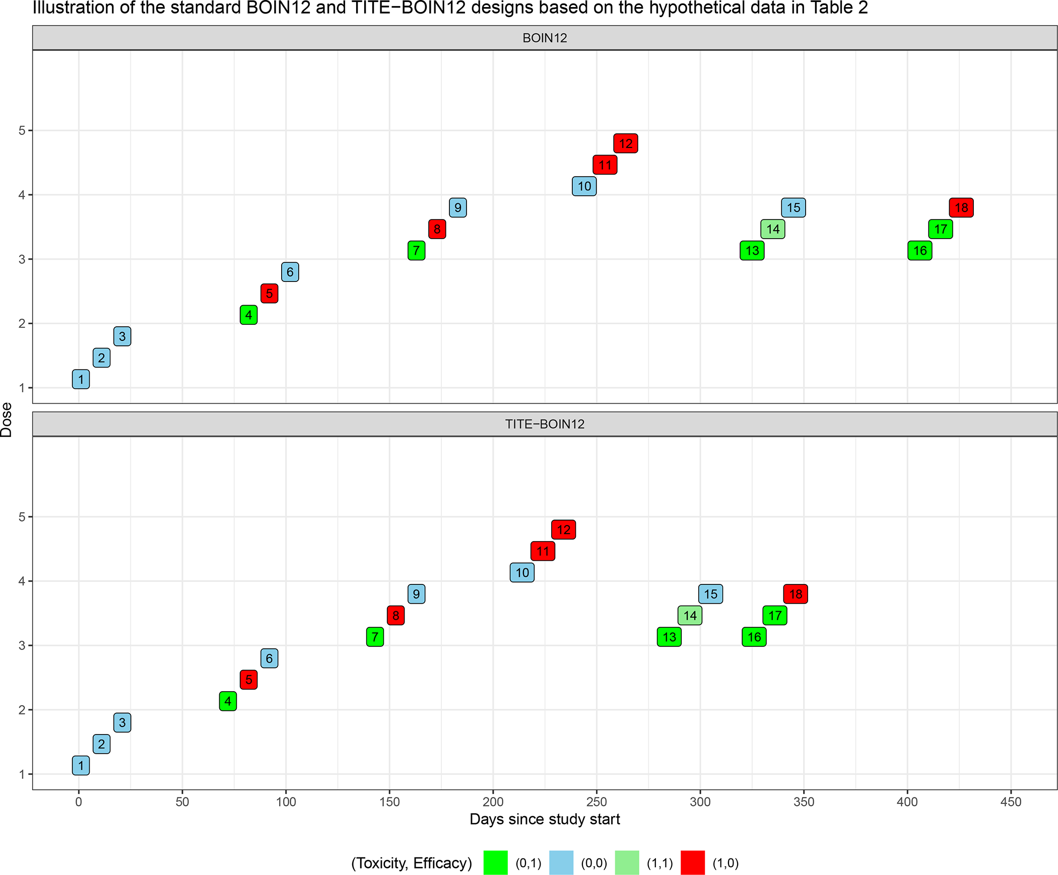
Trial illustration by applying the standard BOIN12 design and the TITE-BOIN12 design.

TABLE 2.

Hypothetical patient-level data for trial illustration

BOIN12							TITE-BOIN12
ID	Dose	YT	YE	Day	XT	XE	ID	Dose	YT	YE	Day	XT	XE
1	1	0	0	1	-	-	1	1	0	0	1	-	-
2	1	0	0	11	-	-	2	1	0	0	11	-	-
3	1	0	0	21	-	-	3	1	0	0	21	-	-
4	2	0	1	82	-	40	4	2	0	1	72	-	40
5	2	1	0	92	30	-	5	2	1	0	82	30	-
6	2	0	0	102	-	-	6	2	0	0	92	-	-
7	3	0	1	163	-	40	7	3	0	1	143	-	40
8	3	1	0	173	25	-	8	3	1	0	153	25	-
9	3	0	0	183	-	-	9	3	0	0	163	-	-
10	4	0	0	244	-	-	10	4	0	0	214	-	-
11	4	1	0	254	40	-	11	4	1	0	224	40	-
12	4	1	0	264	35	-	12	4	1	0	234	35	-
13	3	1	1	325	25	30	13	3	1	1	285	25	30
14	3	0	1	335	-	55	14	3	0	1	295	-	55
15	3	0	0	345	-	-	15	3	0	0	305	-	-
16	3	0	1	396	-	50	16	3	0	1	316	-	50
17	3	0	1	406	-	50	17	3	0	1	326	-	50
18	3	1	0	416	30	-	18	3	1	0	336	30	-

ID: patient ID; Day: day of enrollment.

For the TITE-BOIN12 design, at day 71, when two patients of the first cohort complete endpoint assessment (e.g., < 50% of patients have pending data), we estimate the dose desirability for dose 1, which is 0.113 (Table S.3). As dose 1 is safe and the desirability is less than 0.295 at dose 2, we escalate to dose 2 to treat patients 4–6. If BOIN12 were used, we would wait for 10 more days to have all outcomes observed for the first cohort before enrolling the second cohort. With TITE-BOIN12, dose escalation continues until the fourth cohort. At day 284, patients 10 and 11 complete their assessment and patients 11 and 12 experience a DLT at dose 4. This dose is deemed overly toxic and TITE-BOIN12 de-escalates back to dose 3 to treat patients 13–15. At day 315, four out of the six patients treated at dose 3 complete evaluation for both efficacy and toxicity. TITE-BOIN12 proceeds to estimate the desirability for all the doses used to treat patients based on all observed data. Dose 3 appears to have the highest desirability among the tried dose levels, and it is used to treat the next cohort (patients 16–18) starting on day 316. If BOIN12 were used, it would take 396 days to get to this point. With the use of TITE-BOIN12, on day 396, all patients complete the efficacy and toxicity assessment. The trial duration would be 476 days with use of BOIN12. The estimated desirability for doses 1, 2, 3, and 4 are 0.113, 0.156, 0.208, and 0.022, respectively. Because nine patients are treated at dose 3, the decision is to stay on this dose, we stop the trial. Dose 3 is estimated to have the highest utility and thus declared as the OBD.

3 |. SIMULATION

3.1 |. Scenario configuration

We carried out simulation studies to evaluate the operating characteristics of the TITE-BOIN12 design based on the setting of the renal cell carcinoma trial. We considered five dose levels. The highest acceptable DLT probability was ϕ_T = 0.35, and the lowest acceptable efficacy probability was ϕ_E = 0.25. The utility example 1 in Table 1 was used to define toxicity-efficacy trade-off. Patients were treated in cohorts of three with a maximum sample size of 36. The accrual rate was three patients per month. The toxicity and efficacy assessment windows were 45 days and 60 days, respectively. The probability cutoffs in admissibility criteria (5) and (6) were set as c_T = 0.95 and c_E = 0.90, respectively. We examined 18 representative scenarios (Table S.4) with various dose-response curve shapes. All doses in Scenarios 17 and 18 are toxic, and all doses in Scenario 17 are futile. Figure 2 visualizes the first nine scenarios with MTDs and OBDs marked on the DLT probability curve and utility curves, respectively. Note that only Scenarios 3 and 4 have an OBD that coincides with their MTD. Under each scenario, we generated (Y_T ,Y_E) based on a Gumbel model:

$$\begin{gathered} \mathrm{Pr}\left(Y_T=a,Y_E=b\right)={\pi }_T^a{\left(1-{\pi }_T\right)}^{1-a}{\pi }_E^b{\left(1-{\pi }_E\right)}^{1-b} \\ +{\pi }_T\left(1-{\pi }_T\right){\pi }_E\left(1-{\pi }_E\right){(-1)}^{{}^{a+b}}\left(\frac{exp(c)-1}{exp(c)+1}\right), \end{gathered}$$ (12)

where a, b ∈ {0, 1}, and c is the association parameter between π_T and π_E. We present the results when c = 0 in this section and examine the sensitivity of the design to c in the next section. We compared TITE-BOIN12_BDA and TITE-BOIN12_AL with BOIN12 and EffTox. We chose EffTox as a comparator because it is a well-known model-based design, and it is one of few phase I/II designs that have been implemented in practice.²⁸ The EffTox design parameters were calibrated to ensure a comparable toxicity-efficacy trade-off to that of the TITE-BOIN12 design. Specifically, to determine the equivalence contour in the EffTox design, we specified the three equivalent pairs of (efficacy probability, DLT probability) as (0.6, 0), (1, 0.6), and (0.77, 0.25). Based on the specified utilities values (Ψ₀₁, Ψ₀₀, Ψ₁₁, Ψ₁₀) = (100, 40, 60, 0) for the TITE-BOIN12 design, all the three pairs of the equivalent points in EffTox had a utility value of 76. All of the designs started the trial at the lowest dose level (Section S.10 provides results for the designs when the starting dose level was 3). All designs imposed the same dose elimination rules.

FIGURE 2.

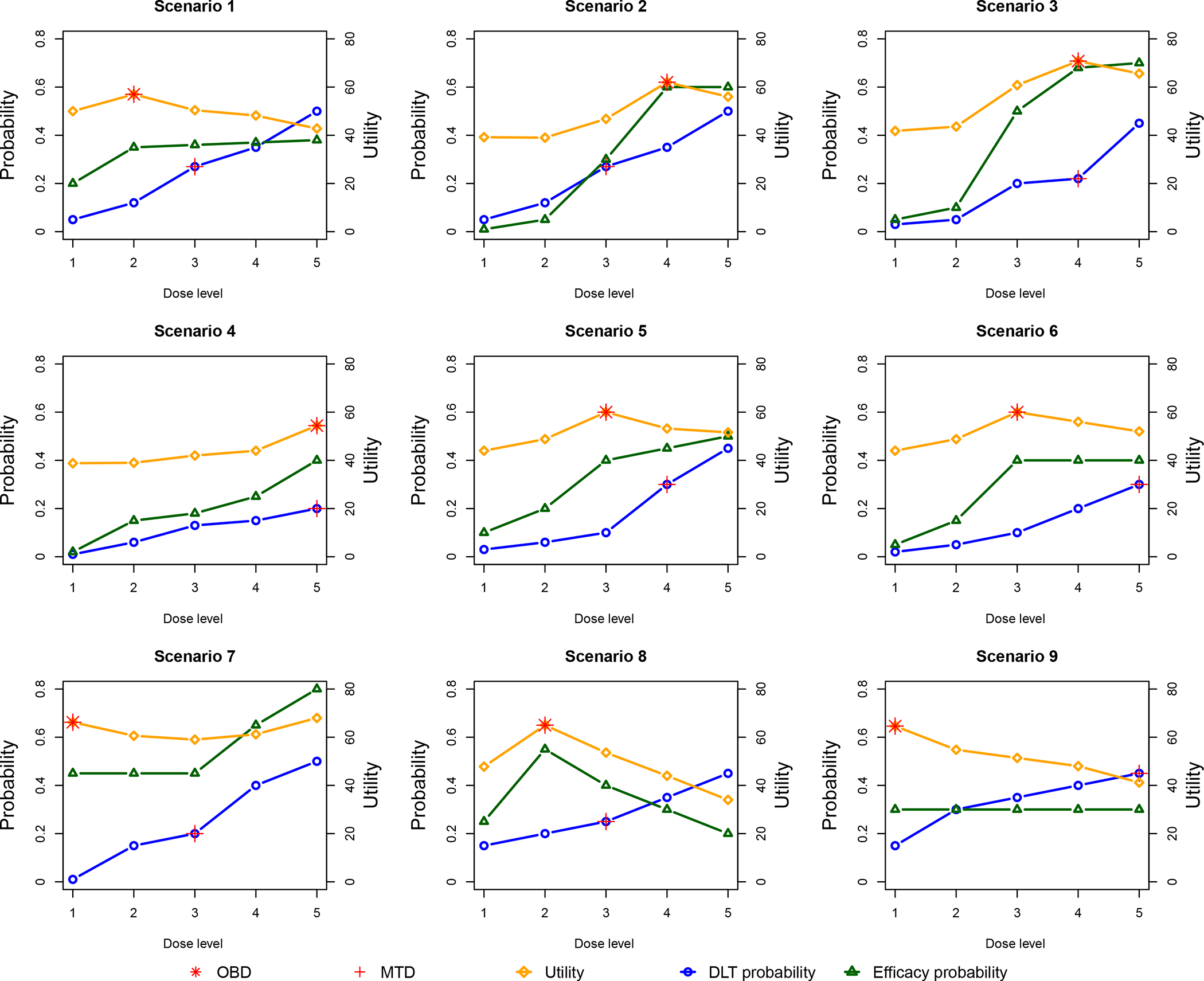
The nine representative scenarios for simulation study.

3.2 |. Operating characteristics

To quantify the operating characteristics (OCs) of the designs, we consider four metrics for comparison: A) percentage of correct selection of the OBD, B) number of patients treated at OBD, C) number of patients treated at overdoses (i.e., with DLT probability > 0.35), and D) trial duration. Metrics A and B measure the accuracy of OBD identification and patient allocation, with the higher values demonstrating better performance. Metric C measures the safety of a design (i.e., how likely a design is to assign patients to excessively unsafe or in-efficacious doses), and metric D measures the efficiency of a design in terms of time used to complete a trial. For both metrics C and D, lower values indicate better performance.

The simulation results are shown in Figure 3. Overall, both TITE-BOIN12_BDA and TITE-BOIN12_AL have comparable performance to BOIN12 in terms of metrics A-C, and they have much shorter trial durations (a desirable outcome for D). Therefore, in what follows, we will focus the comparison of the OCs between TITE-BOIN12_AL and the model-based EffTox, where more differences are observed.

FIGURE 3.

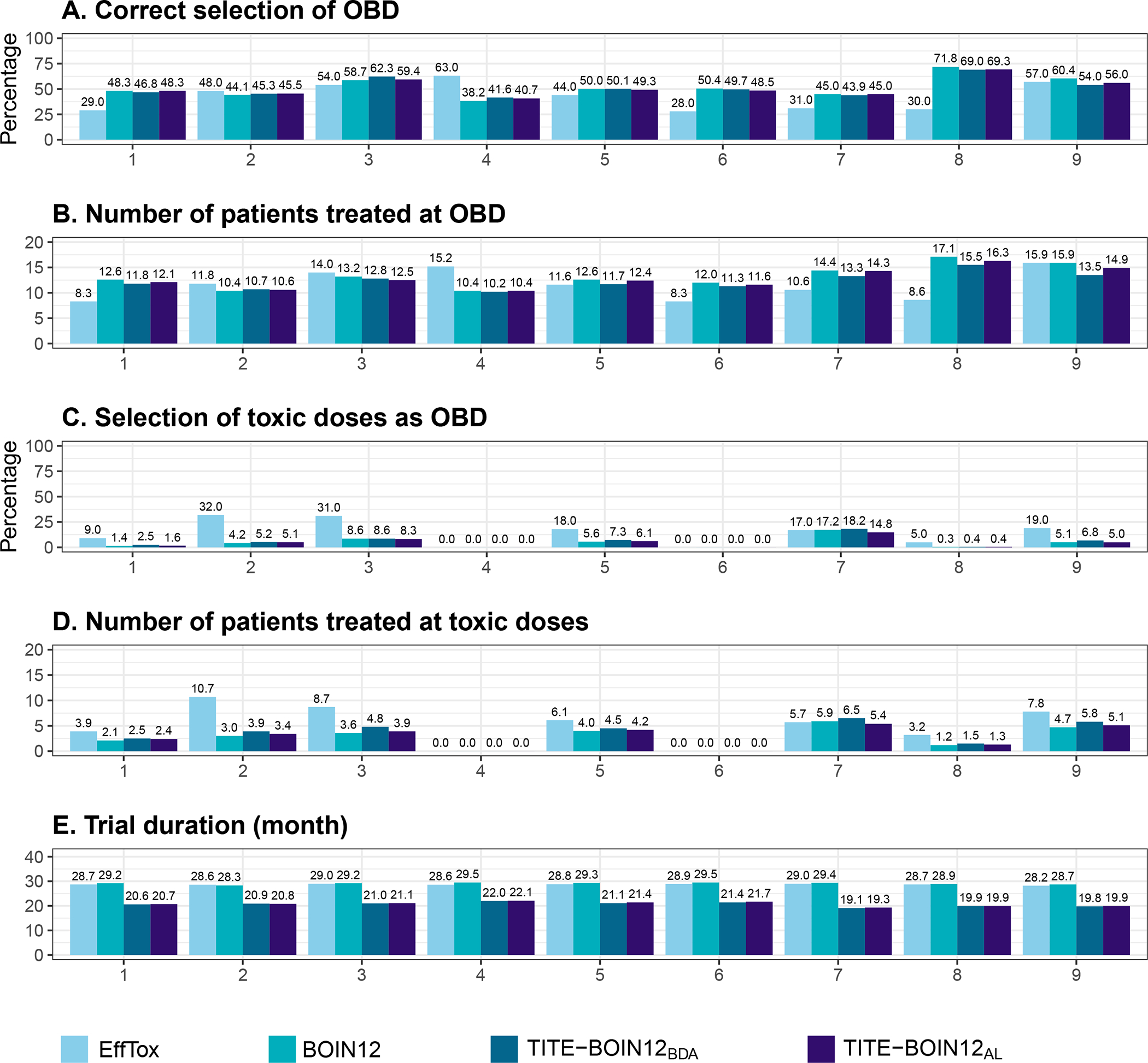
The operating characteristics include (A) percentage of correct selection of the OBD, (B) number of patients treated at OBD, (C) percentage of selecting toxic doses as OBD, (D) number of patients treated at overdoses (with DLT probability > 0.35), and (E) trial duration, based on the EffTox, BOIN12, TITE-BOIN12_BDA, and TITE-BOIN12_AL designs. The results were based on 2,000 simulated trials using each of the nine scenarios shown in Figure 2. The maximum sample size was 36.

Scenario 1 considers the case that the dose-efficacy curve first increases and then nearly plateaus at OBD (i.e., dose level 2). TITE-BOIN12_AL greatly outperforms EffTox in that it has a 17% greater chance of correct OBD selection and assigns more patients to OBD (12.1 versus 8.3). In terms of trial duration, TITE-BOIN12_AL takes about 8 months fewer than EffTox in all the scenarios. In Scenario 2, dose 3 is MTD, but dose 4 is OBD with the highest utility. The model-based EffTox design is much more aggressive and treats slightly more patients at OBD with a 2.5% higher percentage of correct selection, but this is at the cost of overdosing seven more patients. Scenarios 3 and 4 have an OBD that coincides with their MTD, which is located at dose level 4 and 5, respectively. We note that EffTox outperforms TITE-BOIN12 by having more patients allocated to OBD, especially in Scenario 4 where OBD is the highest dose. In this case, EffTox has greater selection. The same finding is observed in Scenario 14, where the highest dose is OBD. The relative superiority of EffTox in Scenarios 4 and 14 is actually due to the aggressiveness of EffTox (Figures S.4–S.5). In Scenario 5, dose 3 is much safer than dose 4 in terms of the DLT probability, but the efficacy improvement from dose 3 to dose 4 is minimal, making dose 3 OBD. TITE-BOIN12_AL has a 5% higher chance to correctly select OBD, treats more patients at OBD, and is still safer than EffTox. The OBDs in Scenarios 6 and 7 are two doses lower than their respective MTDs. In these two scenarios, the OBD selection percentage of TITE-BOIN12_AL is substantially greater than that of EffTox (e.g., 48.5% versus 28% in Scenario 6). For Scenario 7, the OBD is the lowest dose with a high efficacy probability and a particularly small toxicity rate. Although dose 4 has a much higher efficacy probability, it is overly toxic. In this case, TITE-BOIN12_AL has a 14% greater probability of identifying OBD and allocates four more patients to OBD. In Scenario 8, the dose-efficacy curve has an umbrella shape: the efficacy probability first rises from dose 1 to dose 2 and then decreases as dose level increases. The correct selection percentage of the TITE-BOIN12_AL design is more than twice that of EffTox (i.e., 69.3% versus 30%). And eight more patients are treated at OBD with TITE-BOIN12_AL, while the design remains at a lower risk of overdosing. This demonstrates the flexibility of TITE-BOIN12_AL in accommodating various dose response curves. Scenario 9 considers a special case where the efficacy probability plateaus from dose level 1 at 0.3, making the first dose OBD. TITE-BOIN12_AL and EffTox have comparable correct selection of OBD and number of patients at OBD, but EffTox still appears more aggressive and allocates more patients to overly toxic doses. In the case where all doses are toxic (Scenarios 17 and 18) regardless of whether or not the doses are futile, all of the designs have comparable performance (Figures S.4–S.5). In general, we note that EffTox is more likely to select a toxic dose as OBD, which is substantial in Scenarios where the utility does not increase with dose levels (e.g., Scenarios 9 and 16).

Due to the simplicity, accuracy, and robustness of TITE-BOIN12_AL, we recommend it for practical use. The TITE-BOIN12 design, by default, thus refers to TITE-BOIN12_AL.

4 |. SENSITIVITY

We conducted extensive sensitivity analyses to assess the performance of the TITE-BOIN12 design. To investigate the sensitivity of TITE-BOIN12 to the correlation between DLT and efficacy probabilities, we varied the correlation coefficient c in the Gumbel model from 0 to 0.6. Figure S.2 shows the difference between using c = 0 and c = 0.6, where the difference is calculated by (metric value when using c = 0) − (metric value when using c = 0.6). As shown, TITE-BOIN12 yields robust performance in all metrics considered across different correlations. For example, the absolute mean difference in the percentage of correct selection of OBD is only 0.5 across the nine scenarios and the mean difference in the number of patients treated at OBD is 0.1.

One major advantage of TITE-BOIN12 is that it can incorporate the risk-benefit trade-off into the design by eliciting utility values from clinicians. We examined the performance of TITE-BOIN12 given different elicited utility values. Figure S.2 shows the difference of the OCs between two sets of utilities Ψ ∈ {Ψ₁ = (100, 40, 60, 0),Ψ₂ = (100, 40, 70, 0)}. The difference is calculated by (metric value when using Ψ₁) − (metric value when using Ψ₂). As shown, the OCs have some negligible changes. For instance, the mean difference in the percentage of correct selection of OBD is 1.3%, and there is no difference in other matric values.

The expected utility u was modeled using a quasi-binomial model in TITE-BOIN12. We also considered using an exact posterior cumulative distribution function (CDF) of u to serve as the gold standard to assess the accuracy of using the quasi-binomial model. The CDF of u given observed data D is determined by

$$F_u\left(u_b\mid D\right)=\underset{\Theta }{\int }f\left(p_{01},p_{00},p_{11},p_{10}\mid D\right)I\left(u\le u_b\right)d{p}_{01}d{p}_{00}d{p}_{11}d{p}_{10},$$

where $\Theta =\{\left(p_{01},p_{00},p_{11},p_{10}\right):p_{ab}\ge 0,{\sum }_{a=0}^1{\sum }_{b=0}^1{p}_{ab}=1\}$. Results in Figure S.2 show that the quasi-binomial model has great accuracy, as the absolute mean differences in all metrics’ value ranges from 0 to 0.2. The advantage of the quasi-binomial model is that it greatly simplifies computation, saving a great amount of time (Section S.11). We also examined if TITE-BOIN12 is sensitive to the underlying time-to-event distributions. We assumed that the time to toxicity and efficacy follow a uniform distribution versus a Weibull distribution. Results in Figure S.2 show that TITE-BOIN12 is robust to the underlying time-to-event distributions.

Last but not least, we assessed the design’s performance under different endpoint assessment windows: A = (A_T, A_E) ∈ {A₁ = (45days, 60days), A₂ = (60days, 90days)}. The difference shown for each metric was calculated as (metric value when using A₁) − (metric value when using A₂). As shown in Figure S.2, the results using A₂ are extremely close to that of using A₁ in metrics A-C. As expected, when the assessment windows are shorter, the trial duration is smaller (Figure S.2). As the assessment window increases, it becomes harder for the design as more pending outcomes will exist. To further assess the robustness of the TITE-BOIN12 design to this parameter, we added two sets of longer assessment times for both toxicity and efficacy: A = (A_T, A_E) ∈ {A₁ = (75days, 120days), A₂ = (90days, 120days)}. Figure S.3 shows that while some small variations are observed, TITE-BOIN12 is generally robust.

5 |. SOFTWARE

We developed a user-friendly Shiny web application to facilitate the implementation of the TITE-BOIN12 design, which is freely available at www.trialdesign.org. Users can access the TITE-BOIN12 app under the BOIN suite at the website. The Shiny app is developed with standard operating procedure (SOP) to ensure that the app is reproducible, reliable, and stable. The app includes five functional tabs and has the capability to design a trial, run simulations to assess the design’s operating characteristics, generate a concise protocol template, conduct interim analysis to guide dose assignment for the next cohort of patients, and determine OBD after the trial completes. A detailed example of using this app is provided in Section S.12.

6 |. CONCLUSION

To overcome the logistical difficulty caused by monitoring late-onset toxicity and efficacy, we proposed the TITE-BOIN12 design to enable real-time decision making in the presence of pending outcomes. We considered BDA and the approximated likelihood approach, which yield similar performances. For practical use, we recommend TITE-BOIN12 with the approximated likelihood approach because of its fast computation and simplicity. The TITE-BOIN12 design provides a practical, well-performing solution for utility-based phase I/II trials with late-onset toxicity and efficacy. It supports continuous accrual without sacrificing patient safety or the accuracy of identifying OBD. Compared to the more complicated model-based EffTox design, the model-assisted TITE-BOIN12 is capable of accommodating different shapes of dose-efficacy curves, and it has higher accuracy in identifying OBD in most cases. Moreover, it has better overdose control, while significantly reducing trial duration. When all the pending toxicity and efficacy data become available, TITE-BOIN12 seamlessly reduces to BOIN12.

TITE-BOIN12 has several limitations. First, it focuses on single agent dose-finding trials. Given the importance of drug combination trials, it is of great interest to extend TITE-BOIN to combination trials. One approach is to take the strategy of evaluating the desirability of the doses adjacent to the current dose and selecting the best one as the dose for treating the next cohort of patients.²⁹ The advantage of this approach is that it keeps the simplicity of the design. Secondly, TITE-BOIN12 takes a non-informative approach and assumes a priori that the time to both DLT and efficacy are uniformly distributed over the assessment window to incorporate the information of pending patients. TITE-BOIN12 is robust to this uniform assumption, similar to what is demonstrated in TITE-CRM²⁵ and TITE-BOIN.²⁷ But if reliable prior information is available, different distributions can be used. For example, if we expect that DLT or efficacy are more likely to occur in either the earlier or the later part of the assessment window, we can use a prior distribution with more weights on the earlier or the later part of the assessment window to incorporate that prior information. Lastly, TITE-BOIN12 does not account for patient subgroups, e.g., subgroups defined by the level of PD1 or PD-L1 for immune checkpoint inhibitors. One simple approach to this challenge is to stratify the patients and then apply TITE-BOIN12 to each subgroup independently. A more flexible option is to take a model-based approach (e.g., see Guo and Yuan⁹), which allows information borrowing across subgroups, but at the cost of losing the simplicity of model-assisted designs.

References

- 1.Reynolds AR. Potential relevance of bell-shaped and u-shaped dose-responses for the therapeutic targeting of angiogenesis in cancer. Dose-response 2010; 8(3): dose–response. [DOI] [PMC free article] [PubMed] [Google Scholar]
- 2.Sachs JR, Mayawala K, Gadamsetty S, Kang SP, Alwis dDP. Optimal dosing for targeted therapies in oncology: drug development cases leading by example. Clinical Cancer Research 2016; 22(6): 1318–1324. [DOI] [PubMed] [Google Scholar]
- 3.Thall PF, Russell KE. A strategy for dose-finding and safety monitoring based on efficacy and adverse outcomes in phase I/II clinical trials. Biometrics 1998: 251–264. [PubMed] [Google Scholar]
- 4.O’Quigley J, Pepe M, Fisher L. Continual reassessment method: a practical design for phase 1 clinical trials in cancer. Biometrics 1990: 33–48. [PubMed] [Google Scholar]
- 5.Braun TM. The bivariate continual reassessment method: extending the CRM to phase I trials of two competing outcomes. Controlled Clinical Trials 2002; 23(3): 240–256. [DOI] [PubMed] [Google Scholar]
- 6.Thall PF, Cook JD. Dose-finding based on efficacy–toxicity trade-offs. Biometrics 2004; 60(3): 684–693. [DOI] [PubMed] [Google Scholar]
- 7.Yin G, Li Y, Ji Y. Bayesian dose-finding in phase I/II clinical trials using toxicity and efficacy odds ratios. Biometrics 2006; 62(3): 777–787. [DOI] [PubMed] [Google Scholar]
- 8.Liu S, Johnson VE. A robust Bayesian dose-finding design for phase I/II clinical trials. Biostatistics 2016; 17(2): 249–263. [DOI] [PMC free article] [PubMed] [Google Scholar]
- 9.Guo B, Yuan Y. Bayesian phase I/II biomarker-based dose finding for precision medicine with molecularly targeted agents. Journal of the American Statistical Association 2017; 112(518): 508–520. [DOI] [PMC free article] [PubMed] [Google Scholar]
- 10.Zang Y, Lee JJ, Yuan Y. Adaptive designs for identifying optimal biological dose for molecularly targeted agents. Clinical Trials 2014; 11(3): 319–327. [DOI] [PMC free article] [PubMed] [Google Scholar]
- 11.Zang Y, Lee JJ. A robust two-stage design identifying the optimal biological dose for phase I/II clinical trials. Statistics in medicine 2017; 36(1): 27–42. [DOI] [PMC free article] [PubMed] [Google Scholar]
- 12.Liu S, Guo B, Yuan Y. A Bayesian phase I/II trial design for immunotherapy. Journal of the American Statistical Association 2018: 1–12. [DOI] [PMC free article] [PubMed] [Google Scholar]
- 13.Yuan Y, Nguyen HQ, Thall PF. Bayesian designs for phase I-II clinical trials. CRC Press. 2017. [Google Scholar]
- 14.Lin R, Yin G. STEIN: A simple toxicity and efficacy interval design for seamless phase I/II clinical trials. Statistics in Medicine 2017; 36(26): 4106–4120. [DOI] [PubMed] [Google Scholar]
- 15.Takeda K, Taguri M, Morita S. BOIN-ET: Bayesian optimal interval design for dose finding based on both efficacy and toxicity outcomes. Pharmaceutical Statistics 2018; 17(4): 383–395. [DOI] [PubMed] [Google Scholar]
- 16.Zhou Y, Lee JJ, Yuan Y. A utility-based Bayesian optimal interval (U-BOIN) phase I/II design to identify the optimal biological dose for targeted and immune therapies. Statistics in Medicine 2019; 38(28): S5299–S5316. [DOI] [PMC free article] [PubMed] [Google Scholar]
- 17.Lin R, Zhou Y, Yan F, Li D, Yuan Y. BOIN12: Bayesian optimal interval phase I/II trial design for utility-based dose finding in immunotherapy and targeted therapies. JCO Precision Oncology 2020. [DOI] [PMC free article] [PubMed] [Google Scholar]
- 18.Tanner MA, Wong WH. The calculation of posterior distributions by data augmentation. Journal of the American statistical Association 1987; 82(398): 528–540. [Google Scholar]
- 19.Lin R, Yuan Y. Time-to-event model-assisted designs for dose-finding trials with delayed toxicity. Biostatistics 2019. [DOI] [PMC free article] [PubMed] [Google Scholar]
- 20.Murray TA, Yuan Y, Thall PF, Elizondo JH, Hofstetter WL. A utility-based design for randomized comparative trials with ordinal outcomes and prognostic subgroups. Biometrics 2018; 74(3): 1095–1103. [DOI] [PMC free article] [PubMed] [Google Scholar]
- 21.Houede N, Thall PF, Nguyen H, Paoletti X, Kramar A. Utility-based optimization of combination therapy using ordinal toxicity and efficacy in phase I/II trials. Biometrics 2010; 66(2): 532–540. [DOI] [PMC free article] [PubMed] [Google Scholar]
- 22.Liu S, Yuan Y. Bayesian optimal interval designs for phase I clinical trials. Journal of the Royal Statistical Society: Series C: Applied Statistics 2015: 507–523. [Google Scholar]
- 23.Liu S, Yin G, Yuan Y. Bayesian data augmentation dose finding with continual reassessment method and delayed toxicity. The annals of applied statistics 2013; 7(4): 1837. [DOI] [PMC free article] [PubMed] [Google Scholar]
- 24.Jin IH, Liu S, Thall PF, Yuan Y. Using data augmentation to facilitate conduct of phase I–II clinical trials with delayed outcomes. Journal of the American Statistical Association 2014; 109(506): 525–536. [DOI] [PMC free article] [PubMed] [Google Scholar]
- 25.Cheung YK, Chappell R. Sequential designs for phase I clinical trials with late-onset toxicities. Biometrics 2000; 56(4): 1177–1182. [DOI] [PubMed] [Google Scholar]
- 26.Little RJ, Rubin DB. Statistical analysis with missing data. 793. John Wiley & Sons. 2019. [Google Scholar]
- 27.Yuan Y, Lin R, Li D, Nie L, Warren KE. Time-to-event Bayesian optimal interval design to accelerate phase I trials. Clinical Cancer Research 2018; 24(20): 4921–4930. [DOI] [PMC free article] [PubMed] [Google Scholar]
- 28.Yan F, Thall P, Lu K, Gilbert M, Yuan Y. phase I–II clinical trial design: a state-of-the-art paradigm for dose finding. Annals of Oncology 2018; 29(3): 694–699. [DOI] [PMC free article] [PubMed] [Google Scholar]
- 29.Lin R, Yin G. Bayesian optimal interval design for dose finding in drug-combination trials. Statistical methods in medical research 2017; 26(5): 2155–2167. [DOI] [PubMed] [Google Scholar]
Associated Data
This section collects any data citations, data availability statements, or supplementary materials included in this article.