

Abstract

This paper presents the modeling of a continuous-flow reactor used for the synthesis of organic products. The finite element method software, COMSOL Multiphysics, was used to model transport phenomena and reaction kinetics. The temperature is one of the most important kinetic factors that may modify the reaction. A rise in temperature can generate a positive reaction but also secondary side reactions. The design of our system and of many other continuous systems makes it impossible, however, to measure the temperature throughout the reactor. In this paper, we modeled the temperature profile within the reactors as a function of the flow rate, temperature set point, and type of reactor material. The results demonstrated that although it is not a good thermal conductor, polytetrafluoroethylene can be used like other materials. The desired temperature was not reached for any of the reactor material likely to affect the product yield. The model gave the residence time required to reach the stabilized temperature. The comparison of calculated and experimental values of outlet temperature showed good agreement, with a maximum relative difference of only 5%. Knowledge of the temperature profile made it possible to control the concentration distribution of the chemical species in the reactor. The aldol condensation was chosen to determine the kinetic parameters of this reaction as the products of this reaction are found in many natural molecules and drugs. To integrate the chemical model, the kinetic parameters were determined by using experimental data. An equilibrium concentration of 0.2 mol/L was found with initial reactant concentrations of 0.45 mol/L. The chemical modeling gave the species concentrations throughout the reactor. Calculated concentrations were in good agreement with experimental data, with a maximum relative difference of less than 9%. By modeling this reaction, the reaction yield as a function of reactant concentration, temperature, and residence times was estimated.
Introduction
Batch reactors are traditionally used in chemical production because of their flexibility and versatility.1 However, scale up is always a great challenge during the development of batch technologies. An additional challenge for the pharmaceutical industry is to save time during the preclinical and clinical phase (phase 1). During this phase, drug production must have the same reliability and quality. Continuous processes meet these constraints, and flow microreactors appear well-suited for the relatively low tonnage of the pharmaceutical industry. The goal when using continuous reactors is to create efficient and scalable protocols. Synthesis in microreactors is increasingly addressed in many industrial laboratories including the pharmaceutical and fine chemicals industries.2−10
Microreactors provide a high surface-to-volume ratio, giving good heat transfer which improves selectivity, reduces costs, and maximizes reaction yields and product quality. These capacities make them competitive compared to other intensification processes such as microwaves. Their advantages have been demonstrated in several chemistry fields such as analytical chemistry and organic synthesis chemistry.11−18 However, the temperature profile must be known at all points of the reactor in order to ensure reproducibility and safe conditions.19−22 The current trend in organic chemistry is to use tubular reactors as they allow rapid start-up of the system. In this paper, we determined the thermal profiles within tubular reactors with an internal diameter of 1 mm. These reactors were inserted into the commercial equipment Uniqsis to control the heating and flow of incoming reagents. With this technology, the flow rates and temperature can be easily controlled and the length of the reactor can be selected in order to control the residence time. While it is relatively straightforward to qualify the flow rates, it is difficult to ascertain the temperature as a function of the location in the reactor. The actual temperature is essential information for extrapolation.
Furthermore, the thermal profile within the reactors obviously depends, in addition, on the heating powers applied but also on the reaction enthalpies involved in the chemical syntheses.23−25
In order to carry out a comprehensive study, it is therefore necessary to simulate the system by coupling physical phenomena. This simulation is an important design step because it will allow the optimization of the operating conditions.26 In the present study, COMSOL Multiphysics software was used. COMSOL Multiphysics software is a powerful finite-element method (FEM) and partial differential equation (PDE) solution engine.27 It makes it possible to consider multiple phenomena when developing the model: in our case, heat, mass and momentum transfers, and chemical reactions. Eventually, this modeling will be used to establish a relationship between global parameters and local conditions. This can be used to assess the impact of modifying the operating parameters on the product. It will also be used, after the validation of these conditions, to size the process on an industrial scale by extrapolation. To accomplish the scale-up from laboratory to industrial scale, modeling is an essential tool in addition to experimentation. Various examples of modeling of microreactors are reported in the literature. Some publications study hydrodynamics28 and temperature,7,29−31 whereas others focus on kinetic analysis and the determination of reaction parameters.6,22
For modeling, the aldol condensation was chosen here because of its importance in organic chemistry.32−34 The structural unit of the products formed is found in many natural molecules and drugs,35 and its importance is attested by the abundant literature describing industrially or academically viable continuous-flow systems.36−40
This reaction, like all chemical reactions, is affected by several parameters, such as concentration, rate of addition, temperature, and solvent. The temperature of the reaction medium is one of the most important kinetic factors that may modify the reaction. A rise in temperature can generate a positive reaction but also secondary side reactions.
In this paper, we modeled the temperature profile within the reactors as a function of the flow rate, temperature set point, and type of reactor material. In this study, polytetrafluoroethylene (PTFE) was especially studied as it is often used by chemists. This knowledge was applied to determine the chemical species generated by the aldol condensation at the reactor exit as a function of temperature.
Materials and Methods
The systems considered here were Uniqsis coil reactors (Figure 1). These reactors are tubes with an inner diameter of 1 mm. They can be made of PTFE, perfluoroalkoxy (PFA), stainless steel, or Hastelloy C-276. Table 1 gives some characteristics of these tubes.
Figure 1.

Coil FlowSyn reactor from Uniqsis (material: PTFE) and 3D geometry modeled. Photograph courtesy of Uniqsis Ltd. Copyright 2018.
Table 1. Characteristics of Microreactor Tubes.
| PTFE | PFA | stainless steel | Hastelloy | |
|---|---|---|---|---|
| Pmax (bar) | 20 | 20 | 200 | 200 |
| Tmax (°C) | 150 | 150 | 300 | 300 |
| chemical resistance | excellent | excellent | very good | excellent |
Our reference reactor is integrated in a FlowSyn system. FlowSyn is used for small-scale individual reactions (flow rate up to 20 mL/min).
FlowSyn combines two high-pressure pumps and two reactor (coil and chip reactor) modules in a single compact unit. Only the coil reactor was studied in this paper. The coil reactor consists of a steel cylinder coated by another aluminum cylinder. The tubular reactor is wrapped around the aluminum cylinder. This aluminum cylinder has an inner diameter of 123 mm, an outer diameter of 129 mm, and a height of 110 mm. The heating resistance is placed between the walls of the steel and aluminum cylinders. The temperatures can be programmed and varied according to the desired reaction temperature. The system is isolated by a glass lid with an inner diameter of 145 mm, a thickness of 2.5 mm, and a height of 140 mm. The whole system is placed on a Teflon disk.
To initiate continuous flow reactions, reagents (A and B) are pumped at predetermined flow rates (from 0.02 to 10 mL/min) into the reactor after passing through a mixing T-piece (90° angle). Figure 2 shows schematically the path of the reagents in the FlowSyn system. The reagents are prepared in a mixture of methanol/water with a volume ratio (3:1) used as solvent. The injection can be achieved in two different ways. The first is by continuous introduction. This means that the solution is prepared in vials and aspirated by the pump. The second is by injection through a loop. The advantage of the latter is that only a minimal quantity of reagent needs to be used. In this paper, this mode was selected and a 2 mL loop was used.
Figure 2.

Synthesis procedure.
The aldol reaction can be performed in an acidic or in a basic medium. In our case, sodium hydroxide (NaOH) was selected as the base. The mechanism of this reaction is given in Scheme 1. Reagent A, a ketone, reacts with NaOH to form an enolate. As this reaction is very fast compared to the condensation, it does not influence the reaction kinetics.
Scheme 1. Aldol Condensation.

In the reactor, the reagents A (ketone) and B (aldehyde) react together to form the expected product, C (α,β-unsaturated ketone), and water, D. This reaction is simplified as follows:
The reaction is reversible. Hence, the reagent concentration does not tend toward 0 but toward an equilibrium concentration.
To establish this concentration, we determined the kinetic parameters. Experiments were carried out with three different temperatures: 25, 50, and 100 °C. The initial concentration of A used was equal to the initial concentration of B, approximately equal to 0.91 mol/L. The NaOH concentration was 2.15 mol/L. The flow rates of the pumps were identical, so the concentrations of the initial solutions were divided by a dilution factor of 2. For each temperature, the inlet flow rate was chosen so as to have residence times of 0.5, 1, 2.5, and 5 min for a 5 mL volume reactor.
α,β-Unsaturated ketone, C, and water, D, were collected in a container at the reactor outlet during a time corresponding to twice the reactor volume. To recover product C, the collected liquid was evaporated under pressure to remove water and methanol. To improve the crystallization of product C, water was added to the remaining quantity and stored in the refrigerator. After a few hours, product C was filtered with water to remove the excess reagent, as product C is the only chemical compound insoluble in water. Finally, the α,β-unsaturated ketone, C, was dried under vacuum to remove the water, and the mass produced was weighed to afford (Z)-2-(pyridin-3-ylmethylene)quinuclidin-3-one as a yellow solid. Of course, this method, which is commonly used in laboratories, does not provide instant concentration but provides chemical yields.
To identify compounds, 1H NMR and 13C NMR spectra were recorded on a Bruker DPX 250 or 400 MHz instrument using CDCl3 and DMSO-d6. The chemical shifts are reported in parts per million (δ scale), and all coupling constant (J) values are reported in hertz. The following abbreviations were used for the multiplicities: s (singlet), d (doublet), t (triplet), q (quartet), p (pentuplet), m (multiplet), sext (sextuplet), and dd (doublet of doublets). Melting points are uncorrected. IR absorption spectra were obtained on a PerkinElmer PARAGON 1000 PC, and the values are reported in inverse centimeters. HRMS spectra were acquired in positive mode with an ESI source on a Q-TOF mass by the “Fédération de Recherche” ICOA/CBM (FR2708) platform. Monitoring of the reactions was performed using silica gel TLC plates (silica Merck 60 F 254). Spots were visualized by UV light (254 and 356 nm). Column chromatography was performed using silica gel 60 (0.063–0.200 mm, Merck). The results for (Z)-2-(pyridin-3-ylmethylene)quinuclidin-3-one were as follows: Rf (EA/PE 70/30) 0.30; mp 117–119 °C; 1H NMR (400 MHz, CDCl3) δ 2.05 (td, J = 3.0, 8.0 Hz, 4H, 2×CH2), 2.66 (p, J = 3.0 Hz, 1H, CH), 2.93–3.05 (m, 2H, N–CH2), 3.12–3.24 (m, 2H, N–CH2), 6.99 (s, 1H, C=CH), 7.30 (dd, J = 4.9, 8.0 Hz, 1H, CHAr), 8.48 (dt, J = 1.9, 8.0 Hz, 1H, CHAr), 8.54 (dd, J = 1.7, 4.8 Hz, 1H, CHAr), 9.05 (d, J = 2.1 Hz, 1H, CHAr); 13C NMR (101 MHz, CDCl3) δ 25.83 (2×CH2), 40.27 (CH), 47.56 (2×N–CH2), 121.63 (Calk), 123.49 (CHAr), 130.12 (Cq), 138.65 (CHAr), 146.68 (C=CH), 150.07 (CHAr), 153.12 (CHAr), 205.74 (Cq); IR (ATR diamond, cm–1) ν 2954, 2937, 1702, 1621, 1409, 1098, 700; HRMS (ESI/MS) m/z calcd for C13H15N2O 215.1178 [M + H]+; found 215.1179.
All reagents were purchased from commercial suppliers and were used without further purification.
Modeling Approach
Using COMSOL Multiphysics, the reactor was built using 3D geometry. To define the operating conditions as well as the limiting conditions, it is first necessary to integrate the various parts around the reactor. Figure 1 shows the modeled zone (modeled system) and the different areas of the 3D geometry (steel cylinder, aluminum cylinder, glass lid, air, liquid inside reactor, reactor walls). CFD (computational fluid dynamics) modules were used to solve the continuity, momentum, and energy equations, while the chemical reaction engineering module was used to describe the reagents and products in a reacting system.
The model was developed in two stages. The first step was to define the model under consideration to determine the temperature as well as the flow in order to ensure good representation of the temperatures in the reactor. The second step was the integration of material transfers and the chemical model by incorporating the aldol condensation.
Thermal/Hydrodynamic Model
Fluid flow (incompressible fluid and laminar flow) is described by the Navier–Stokes equations, which predict the fluid velocity and its pressure in the reactor geometry with a classical set of boundary conditions. For the modeling, the following flow rate values were used: 2, 5, and 10 mL/min. At the outlet, we selected atmospheric pressure for reaction temperatures of 40 and 80 °C, and a pressure of 100 psi for a reaction temperature of 120 °C. A pressure of 100 psi was chosen as it corresponds to the pressure applied with a back pressure regulator (BPR). A no-slip boundary condition (i.e., the velocity is set to zero) is specified at the walls. In these conditions, the Mach number is less than 0.3 and the momentum equation can be simplified by assuming an incompressible fluid. The Reynolds numbers (Re) in the reactor tube corresponding to these flows are between 99 and 418, i.e., lower than 2100, which corresponds to a laminar flow. The momentum equation is written in the following form:
| 1 |
By introducing the temperature, the energy equation is written as follows in solid areas. The imposed temperature is defined on the outer boundaries of the steel cylinder (Figure 1) which heats the reactor. This temperature thus corresponds to the set temperature, and we consider that the cylinder has a homogeneous temperature.
The remaining outer boundaries in contact with a Teflon disc were assumed to be adiabatic. This disc was the white disc at the bottom of the reactor shown on Figure 1. At the external glass wall, a convective heat transfer was defined.
| 2 |
In the liquid phase, due to the non-null velocity, the convection term is added to describe the heat transfer in fluids as follows:
| 3 |
The liquid temperature in the reactor inlet is taken at room temperature (293 K). The coupling of heat flows is effective on the internal walls (internal boundaries between two domains), where contact between the different domains is assumed to be perfect. The temperature and the flux density are continuous at the fluid/solid and solid/solid interfaces.
Chemical Model
The type of reaction (endothermic, exothermic, or athermic) remains an important parameter. The thermodynamic properties of the reaction can thus influence the thermal profile in the reactor. The heat released or absorbed by the reaction can change the temperature T. To model chemical reactions and material transfer of species during synthesis reactions, it is necessary to include the reaction heat (Q) in the energy reaction. This heat is calculated from the enthalpy and the reaction rate. It is equal to
| 4 |
The energy equation is written as follows:
| 5 |
The reaction enthalpy was experimentally determined using a calorimeter. The chemical reaction was carried out in the adiabatic calorimeter at constant pressure. The first reagent was introduced into the calorimeter; the equilibrium temperature was denoted T1. Then the second reagent with the temperature T2 was introduced, and a thermal equilibrium was reached at temperature T3. After calculation, we deduced the heat capacity of the calorimeter. In adiabatic conditions, the quantities of heat exchanged were equal to zero. The temperature variations depending on the quantities of reagents were measured with a thermometer, making it possible to determine the reaction enthalpy (H) according to the following relationship:
| 6 |
where Cp is the heat capacity of the system, which is equal to the heat capacity of the solvent (methanol–water mixture with a ratio of 3:1). In our case, the enthalpy of the reaction was −46.84 J/mol. This value is low, and the reaction can be considered to be athermal.
To study the chemical reaction and define the reaction rate, we used the “reaction model” in COMSOL Multiphysics. The changes in chemical species transported by diffusion and convection were modeled using the “transport of diluted species model”.
Due to the large flow of methanol/water in the system, the diffusion of each species was considered alone in the solvent. Mixture properties such as density and viscosity were assumed to correspond to those of methanol/water (3:1) and were estimated from the methanol and water charts.
The species conservation equation can then be written in the following form:
| 7 |
where Ci(f) refers to the concentration of chemical species i and Di,solvent is the diffusion coefficient of this species in the predefined phase (methanol/water (3:1)).
The production term ri corresponds to the production or consumption reaction of the species i.
For the aldol reaction, the general form of (A + B ⇆ C + D) can be simplified and written in the following form (water D is a solvent):
We note k1 is a kinetic constant in the forward direction and k′2 in the opposite direction, but k′2 is an apparent rate constant.
The rate of the reaction is written in the following form:
| 8 |
This expression is simplified by taking simple initial conditions. The concentrations of A and B are equal, and the order of the reaction is 2/1. The reaction rate can be written in the form:
| 9 |
When t goes to infinity (to equilibrium)
| 10 |
The kinetic expression becomes
| 11 |
The integration and the initial conditions (t = 0, x = 0) give
| 12 |
Kinetic analysis leads to k1. At equilibrium, the measurement of the concentrations gives
| 13 |
The equilibrium constants k1 and k′2 follow the Arrhenius law. They are equal to
| 14 |
| 15 |
After determining k1 and k′2 for different temperature values (25, 50, and 100 °C), the plotting of ln k1 and ln k′2 as a function of ln(1/T) gave the activation energy values E1 and E2 and the Arrhenius factors A1 and A2, respectively.
Kinetic Parameters
To study this reaction, we used 2-benzylidenequinuclidin-3-one derivatives as models due to their potential to generate diagnostic or therapeutic agents.41 3-Quinuclidinone hydrochloride (A) and 3-pyridinecarboxaldehyde (B) were used as reagents. (2Z)-2-(Pyridin-3-ylmethylene)quinuclidin-3-one is the product (C) formed (Scheme 2).
Scheme 2. (2Z)-2-(Pyridin-3-ylmethylene)quinuclidin-3-one Production.

To establish the kinetic constants using the injection mode, the initial concentrations of A and B in the mixture of MeOH/H2O (3:1; v/v) were both 0.91 mol/L. This produces a concentration of 0.45 mol/L for each reagent at the reactor inlet. After passing through the reactor, the concentrations of C and A were determined. The flow rate was decreased until the weight of C was constant, corresponding to an equilibrium concentration. From this result, an average concentration (Cavg) was calculated by dividing this weight by reactor volume. FlowSyn was fitted with a 100 psi BPR. In Table 2, we report the values of Cavg at equilibrium (C*avg) and Cavg for a total flow rate of 10 mL/min, giving a residence time of 0.5 min (C0.5avg). This time is shorter than the equilibrium time. The experiments were carried out at 25, 50, and 100 °C with a 5 mL reactor in PTFE. These values were implemented in eqs 12 and 13 to obtain pseudo-equilibrium constants (k1 pseudo,k′2 pseudo,K′pseudo).
Table 2. Kinetic Constants of the Aldol Reaction.
| temperature (°C) | C0.5avg (mol/L) | C*avg (mol/L) | k1 pseudo (m3/(s·mol)) | k′2 pseudo (s–1) | K′pseudo (m3/mol) |
|---|---|---|---|---|---|
| 25 | 0.145 | 0.215 | 7.90 × 10⁻⁵ | 0.022 | 3.57 × 10⁻³ |
| 50 | 0.151 | 0.214 | 8.31 × 10⁻⁵ | 0.023 | 3.56 × 10⁻³ |
| 100 | 0.161 | 0.215 | 8.98 × 10⁻⁵ | 0.025 | 3.58 × 10⁻³ |
The experimental conditions as well as the calculated kinetic constant values are given in Table 2.
In our conditions, the values of direct and opposite constants did not change much with the temperature. Therefore, the reaction rate is almost constant, which shows the limited influence of temperature in this temperature range. This weak influence can be explained by the low reaction enthalpy determined experimentally and found to be −46.84 J/mol. The values of kinetic constants were obtained by plotting ln k as a function of 1/T. Figure 3 gives straight lines with slopes equal to −E/R and intercepts equal to ln A.
Figure 3.

Kinetic parameter plots.
The calculated values are displayed in Table 3.
Table 3. Activation Energy and Arrhenius Factors.
| kinetic constant | activation energy, E (J/mol) | Arrhenius factor, A (m3/(mol·s)) |
|---|---|---|
| k1 pseudo | 1.58 × 10³ | 1.5 × 10⁻⁴ |
| k’2pseudo | 1.52 × 10³ | 4.1 × 10⁻² |
Results and Discussion
Thermal/Hydrodynamic Model
The simulation was conducted with water as liquid for reasons of usability and data availability. The distribution of the temperature and the hydrodynamics of the liquid at each point of the reactors were determined with a stationary study. Figure 4 shows the radial water evolution temperature inside the 20 mL reactor (PTFE, length = 25 m) for temperature set points of 40, 80, and 120 °C and a water flow of 2, 5, and 10 mL/min. These profiles are the results of CFD. The CFD results are strongly dependent on the mesh quality of the 3D geometry, itself dependent on the number of mesh elements.42 We increased the number of mesh elements until no significant change in the temperature profile was observed. We retained the temperature profiles obtained with 1776164 mesh elements and swept until 2223038 mesh elements. We applied an extremely fine mesh especially in the reactor geometry. In this domain, the mesh size was between 2.5 and 0.225 mm.
Figure 4.
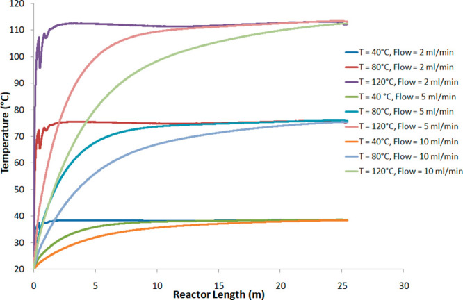
Variation in calculated temperature as a function of the length of the PTFE reactor for T = 40, 80, and 120 °C and water flow = 2, 5, and 10 mL/min.
The water entered at a temperature of 20 °C, and the temperature increased as it progressed through the reactor.
The results showed that, in all cases, the stabilized temperature never reached the set point for reactor lengths of at least 25 m, corresponding to a 20 mL reactor. This means that if the heater of the Uniqsis system reaches the temperature set point, it cannot transmit enough energy to allow the temperature inside the reactor to reach the temperature set point. Table 4 gives the thermal gradient between heating and stabilized temperature. This evolution can be associated with the increase in heat loss at the glass/air surface.
Table 4. Thermal Gradient between Heating and Stabilized Temperature.
| heating temperature (°C) | 40 | 80 | 120 |
|---|---|---|---|
| average stabilized axial temperature (°C) | 38.6 | 75.8 | 113.0 |
| absolute error (°C) | –1.4 | –4.2 | –7 |
| water flow rate (mL/min) | length to reach 99% of the stabilized temperature (m) – corresponding reactor volume (mL) | ||
| 2 | 1.60–1.26 | 1.9–1.50 | 2.0–1.57 |
| 5 | 13.6–10.69 | 16.3–12.80 | 17.2–13.5 |
| 10 | 22.0–17.28 | 23.0–18.06 | 23.6–18.54 |
For a given flow rate, the stabilized temperature values are almost similar, in particular, at 40 and 80 °C. At 120 °C, 1 °C of difference is observed. However, the time, reactor length, or the reactor volume needed to reach this temperature is dependent on the flow. Thus, for a flow rate of 2 mL/min, the time to reach 99% of the temperature stabilization is less than 1 min, requiring a reactor volume of at least 2 mL. For flows of 5 and 10 mL/min, this time is less than 3 and 2 min, requiring reactor volumes of 14 and 20 mL, respectively.
Knowing the residence time makes it possible to select the flow rate or reactor in order to ensure the desired temperature which is, as already mentioned, an important parameter in kinetic reactions. This knowledge also reduces error in the case of scale-up or change of setup.
To study the radial temperature, temperature distributions for three positions (0, r/2, and −r/2) in the reactor tube were calculated. The programmed temperature was 80 °C, and the water flow was 5 mL/min. Results show that the radial temperature within the reactor is homogeneous. The thermal gradient is low (less than 1 °C) and can be neglected. This is one of the advantages of a microreactor: a uniform temperature distribution due to its small size.
Model Validation
To validate the thermal/hydrodynamic model, an experimental study of the temperature distribution in the reactor was carried out to evaluate the difference between the measured and the simulated values. For this study, water was used as a liquid circulating in the reactor. The reactor outlet is the only position that can be used to measure the temperature. Various reactor volumes (5, 10, and 20 mL) were used. This method made it possible to have the temperature at three different points for a fixed water flow. A K thermocouple was used (diameter of 0.5 mm). The comparison was performed by varying the temperature set points (50 and 80 °C) and the water flow (5, 10, and 20 mL/min). Due to the vaporization temperature of water, the temperature is limited to 80 °C. Table 5 shows the simulation results and the experimental measurements of the temperature at the reactor outlets.
Table 5. Outlet Reactor Temperatures (Measured (Tm) and Calculated (Tc)) for Temperature Set Points of 40 and 80°C.
| temperature
(°C) |
|||||||
|---|---|---|---|---|---|---|---|
| 40 |
80 |
||||||
| reactor volume (mL) | water flow (mL/min) | Tm (°C) | Tc (°C) | absolute error (°C) | Tm (°C) | Tc (°C) | absolute error (°C) |
| 20 | 5 | 37.8 | 37.8 | 0 | 73.1 | 73.9 | +0.8 |
| 10 | 37.3 | 37.8 | + 0.5 | 70.8 | 74.1 | +3.3 | |
| 20 | 36.5 | 37.7 | +1.3 | 69.8 | 73.9 | +4.1 | |
| 10 | 5 | 37.2 | 38 | +0.8 | 71.4 | 74.1 | +2.7 |
| 10 | 36.6 | 38.1 | +1.5 | 69.9 | 73.2 | +3.3 | |
| 20 | 35.2 | 36 | +0.8 | 64.6 | 67.5 | +2.9 | |
| 5 | 5 | 36.9 | 38 | +1.1 | 70.4 | 73.7 | +3.3 |
| 10 | 35.9 | 36.5 | +0.6 | 66.4 | 69.1 | +2.7 | |
| 20 | 33.5 | 33.4 | –0.1 | 58.9 | 59.5 | +0.6 | |
| MAEa (°C) | 0.75 | MAE (°C) | 2.64 | ||||
| relative error (%) | 1.9 | relative error (%) | 3.3 | ||||
| RMSEb (°C) | 0.88 | RMSE (°C) | 2.86 | ||||
 .
.
The comparison between the measured and calculated values revealed positive absolute errors, meaning that the model overestimates the values and that the real system is less efficient than the theoretical model. The mean absolute error (MAE) and root mean square error (RMSE) values were almost identical, meaning that the absolute errors have the same magnitude. For a set temperature of 40 °C, the MAE was less than 1 °C against 3 °C for a temperature of 80 °C, representing, respectively, a relative error of 1.9 and 3.3%. However, these relative differences can be neglected, and the model was therefore validated.
Water was used as an example of the liquid for illustration purposes in the above results. However, some chemical reactions need to use organic solvents. To demonstrate the validity of the model for other liquids, ethanol and toluene, the temperature profiles at the reactor center were determined. Figure 5 shows the radial temperature distribution for these liquids for a temperature set point of 80 °C and a liquid flow rate of 5 mL/min. For the three liquids, the stabilized temperatures were almost 75.5 °C. Ninety-nine percent of this value was reached for reactor lengths of 4.9 m (3.85 mL) and 7.5 m (5.89 mL) for toluene and ethanol, respectively, against 16.3 m for water (Table 3). This result can also be expressed in the following way. If a reactor of 20 mL and a flow rate of 5 mL/min are applied, 99% of the liquid is at the stabilized value for 75.5, 62.5, and only 18.5% of the residence time for toluene, ethanol, and water, respectively. This difference is explained by the different isobaric heat capacity of each liquid (1.70, 2.57, 4.18 kJ/kg·K) and by the difference in the thermal conductivities (0.134, 0.167, and 0.606 w/m·K (at 25 °C and 1 bar)) for toluene, ethanol, and water, respectively. The comparison of these temperatures with experimental ones showed good agreement. The maximum relative error was 3.6 and 4.5%, respectively, for toluene and ethanol.
Figure 5.

Variation in temperature versus reactor length for water, ethanol, and toluene (temperature set point: 80 °C; flow rate: 5 mL/min).
Tube Material Effect
To finalize this thermal/hydrodynamic study, the effect of the reactor material was determined. As indicated in the reactor description given above, other materials can be used for the construction of the reactor tube with 1 mm internal diameter and 1.6 mm external diameter. We studied the effect of the material on the temperature distribution in the reactor with a fixed flow rate of 5 mL/min. Figure 6 shows the modeled axial water temperature according to the length of the tube for three different heating temperatures (40, 80, and 120 °C) using PTFE, Hastelloy, and stainless steel as reactor materials.
Figure 6.

Axial temperature distribution for different tube construction materials for three different temperature set points with a water flow rate of 5 mL/min.
A slight thermal gradient was detected with the PTFE curve at the beginning of the curves, especially at high temperature with a maximum deviation of 5 °C. However, the stabilization temperature remained almost the same for the three materials (Figure 6) especially at 80 and 40 °C. At 120 °C, the stabilized temperature for steel and Hastelloy was 1.5 °C higher than that of PTFE. Therefore, for this reactor configuration, PTFE remains a suitable material despite its weak thermal conductivity of 0.259 W/m·K at 50 °C (50.2 and 9.1 for steel and Hastelloy, respectively).
Chemical Model Integration and Exploitation
After validation of the thermal/hydrodynamic model, the next step was the integration of the chemical model. For the following results, a PTFE reactor with a volume of 5 mL was used.
In the injection mode, the profile of the concentrations depends on the residence time distribution, which depends on the molecular axial dispersion. To avoid determining this value, we chose to model with a mode corresponding to a continuous injection of reactants. The model leads to a steady state where there is no axial dispersion due to any concentration gradient.43
Owing to the kinetic constants obtained (Table 2), a simulation was carried out with a 50 °C temperature set point and an inlet flow rate of 2 mL/min. Figure 7 shows the axial concentrations of A, B, and C but also the equilibrium concentrations. The equilibrium concentration of C was 0.2 mol/L, and the equilibrium time was 95 s, corresponding to a reactor length of 4 m (or reactor volume = 3.14 mL). This value is in agreement with the experimental concentration measured under the same conditions (0.2 mol/L).
Figure 7.

Axial concentrations of compounds (CA, CB, CC) for operating conditions: T = 50 °C, flow = 2 mL/min; experimental point (CC exp); and axial profile temperature (T).
To study the effect of temperature and flow rate, the evolution of product concentration (C) was modeled as a function of the length of the reactor. Figure 8 shows the concentration of C at 50 and 100 °C at different flow rates. For the same flow rate, the concentration profiles are quite similar for both temperatures. This result is in agreement with kinetic results as the reaction is almost athermal. Figure 8 shows that a reactor volume of 5 mL does not enable the equilibrium concentration to be reached for a 10 mL/min flow rate, thus revealing the importance of the reactor size.
Figure 8.

Axial product concentration profile (CC) for different flow rates (2.5 and 10 mL/min) and temperature set points (50 °C, 100 °C) for an equal concentration of reagents (0.45 mol/L).
The experimental outlet concentration values of product C for a temperature set point of 100 °C and for three flow rates, 2, 5, and 10 mL/min (residence times equal to 2.5, 1, and 0.5 min, respectively), are given in Figure 8. The relative differences were 4, 5, and 9% for residence times of 2.5, 1, and 0.5 min, respectively. For residence times greater than 1 min, the differences were less than 5%. For a residence time of 0.5 min, the relative error was higher. This could be due to the rapidity of the reaction and the difficulty controlling it for a very low residence time. The values remained below 10% and can be considered negligible. Hence, the model is validated.
The model allows the operating parameters to be varied in order to anticipate the responses. In this part, therefore, we studied the effect of the input reactant concentrations on product concentration. Only the B inlet concentration was changed. Table 6 gives the results of various simulations. The calculations indicate the maximum yield that can be achieved by changing the operating parameters. The use of an excess of reagent B makes it possible to shift the equilibrium in the direction of consumption of A and B and thus, in the direction of production of the product C. The calculations can thus predict a reaction yield. For example, the modeling of an excess of B can increase the yield up to 92%.
Table 6. Simulation Results.
| initial concentration of A (mol/L) | 0.91 | ||||
| inlet flow (mL/min) | 2 | ||||
| temperature (°C) | 100 | 50 | 50 | 50 | 50 |
| initial concentration of B (mol/L) | 0.45 | 0.45 | 2*0.45 | 3*0.45 | 4*0.45 |
| C*avg (mol/L) | 0.2 | 0.2 | 0.3 | 0.34 | 0.36 |
| residence time to achieve Ceq (s) | 75 | 87 | 60 | 31 | 24 |
| predicted yield (%)a | 54 | 54 | 82 | 92 | 92 |
Conclusion
This paper discussed the development of a continuous reactor model to predict the spatial distribution of the resulting species during synthesis. The kinetic models were integrated into the mass, heat and momentum transport model using the COMSOL Multiphysics software. This model showed the effect of the geometry and the characteristics of reactors on the programmed temperature. The models proved capable of predicting the reactor length necessary to reach the temperature set point as a function of flow rate programmed up to 120 °C for a maximum value of 10 mL/min. A negative deviation of a few degrees was always observed. The temperature set points were never reached. Results showed that the radial temperature in the reactor was very homogeneous. The stabilized temperature depended on several parameters (the flow rate and the physicochemical properties of the liquids). These elements must be considered to ensure that the chemical reaction takes place under the right temperature conditions. Moreover, PTFE reactors are widely used by chemists because of their ease of use. Despite the low thermal conductivity properties of PTFE compared to steel or Hastelloy, the temperature profiles showed that it is able to reach the same order of temperatures as steel or Hastelloy reactors. Finally, experimental results were used to validate the simulation. The temperature profiles in the reactors were found to correspond well with the measurement results. The model was applied to the aldol condensation and allowed the prediction of chemical yield. The calculated average concentration at the reactor outlet was compared with the experimental results. The results were generally in good agreement. Thus, the effect of modifying the operating conditions can be easily studied without the need for several experiments. Modeling offers a remarkable time saving advantage and in the long term will make it possible to easily resize a reactor to the final scale. By modifying the chemical kinetics, the model can be extended to cover more chemical reactions.
Acknowledgments
The authors are grateful the Region Centre-Val de Loire for financial support within the INFLUX project.
Glossary
Nomenclature
- ρ
density (kg/m3)
- v
velocity (m/s)
- μ
dynamic viscosity (Pa·s)
- ρs
solid density (kg/m3)
- T
temperature (K)
- ρf
fluid density (kg/m3)
- kf
fluid conductivity (W/(m·K))
- Q
reaction heat (W/m3)
- r
reaction rate (mol/(m3·s))
- Disolvant
diffusion coefficient of chemical species i (m2/s)
- k1
direct kinetic constant (m3/(s·mol))
- q
reagent B order taken equal to 1
- x
concentration of C at t (mol/m3)
- xeq
concentration of C at equilibrium (mol/m3)
- E1, E2
activation energy (J/mol)
- R
perfect gas constant (J/(mol·K))

velocity derivative as a function of time following the fluid motion
- p
pressure (Pa)
- g
gravitational acceleration (m/s–2)
- Cps
solid heat capacity (J/(kg·K))
- ks
solid conductivity (W/(m·K))
- Cpf
fluid heat capacity (J/(kg·K))
- t
time (s)
- H
reaction enthalpy (J/mol)
- Ci(f)
concentration of chemical species i (mol/m3)
- Cavg
concentration of C at equilibrium inside the reactor volume (mol/m3)
- ri
production or consumption reaction of the species i (mol/(m3·s))
- k2
opposite kinetic constant (s–1)
- p
reagent A order taken equal to 1 (mol/m3)
- s
product C order taken equal to 1
- a
initial concentration of reagents
- K
equilibrium constant (mol/m3)
- A1, A2
Arrhenius factor (m3/mol)
The authors declare no competing financial interest.
References
- Rossetti I. Modeling of continuous reactors for flow chemistry. Flow Chemistry. ChimicaOggi - Chemistry Today 2017, 35, 8–11. [Google Scholar]
- Kockmann N. Modular Equipment for Chemical Process Development and Small-Scale Production in Multipurpose Plants. ChemBioEng. Rev. 2016, 3, 5–15. 10.1002/cben.201500025. [DOI] [Google Scholar]
- Deng Q.; Lei Q.; Shen R.; Chen C.; Zhang L. The continuous kilogram-scale process for the synthesis of 2,4,5-trifluorobromobenzene via Gattermann reaction using microreactors. Chem. Eng. J. 2017, 313, 1577–1582. 10.1016/j.cej.2016.11.035. [DOI] [Google Scholar]
- Adamo A.; Beingessner R. L.; Behnam M.; Chen J.; Jamison T. F.; Jensen K. F.; Monbaliu J.-C. M.; Myerson A. S.; Revalor E. M.; Snead D. R.; Stelzer T.; Weeranoppanant N.; Wong S. Y.; Zhang P. On-demand continuous-flow production of pharmaceuticals in a compact, reconfigurable system. Science 2016, 352, 61–67. 10.1126/science.aaf1337. [DOI] [PubMed] [Google Scholar]
- Degennaro L.; Nagaki A.; Moriwaki Y.; Romanazzi G.; Dell'Anna M. M.; Yoshida J.-i.; Luisi R. Flow microreactor synthesis of 2,2-disubstituted oxetanes via 2-phenyloxetan-2-yl lithium. Open Chem. 2016, 14, 377–382. 10.1515/chem-2016-0041. [DOI] [Google Scholar]
- Li L.; Yao C.; Jiao F.; Han M.; Chen G. Experimental and kinetic study of the nitration of 2-ethylhexanol in capillary microreactors. Chem. Eng. Process.: Process. Int. 2017, 117, 179–185. 10.1016/j.cep.2017.04.005. [DOI] [Google Scholar]
- Chen P.-C.; Fan W.; Hoo T.-K.; Chan L. C. Z.; Wang Z. Simulation guided-design of a microfluidic thermal reactor for polymerase chain reaction. Chem. Eng. Res. Des. 2012, 90, 591–599. 10.1016/j.cherd.2011.09.008. [DOI] [Google Scholar]
- Thomas S.; Orozco R. L.; Ameel T. Microscale thermal gradient continuous-flow PCR: A guide to operation. Sens. Actuators, B 2017, 247, 889–895. 10.1016/j.snb.2017.03.005. [DOI] [Google Scholar]
- Kricka L. J.; Wilding P. Microchip PCR. Anal. Bioanal. Chem. 2003, 377, 820–825. 10.1007/s00216-003-2144-2. [DOI] [PubMed] [Google Scholar]
- Borovinskaya E. S.; Reshetilovskii V. P. Microreactors as the New Way of Intensification of Heterogeneous Processes. Russ. J. Appl. Chem. 2011, 84, 1094–1104. 10.1134/S107042721106036X. [DOI] [Google Scholar]
- Yoshida J.; Nagaki A.; Yamada T. Flash Chemistry: Fast Chemical Synthesis by Using Microreactors. Chem. Chem. - Eur. J. 2008, 14, 7450–7459. 10.1002/chem.200800582. [DOI] [PubMed] [Google Scholar]
- Deng Q.; Shen R.; Zhao Z.; Yan M.; Zhang L. The continuous flow synthesis of 4,5-trifluorobenzoic acid via sequential Grignard exchange and carboxylation reactions using microreactors. Chem. Eng. J. 2015, 262, 1168–1174. 10.1016/j.cej.2014.10.066. [DOI] [Google Scholar]
- Roberge D. M.; Ducry L.; Bieler N.; Cretton P.; Zimmermann B. Microreactor technology: a revolution for the fine chemical and pharmaceutical industries?. Chem. Eng. Technol. 2005, 28, 318–323. 10.1002/ceat.200407128. [DOI] [Google Scholar]
- Andreev D. V.; Makarshin L. L.; Gribovskii A. G.; Yushchenko D. Y.; Sergeev E. E.; Zhizhina E. G.; Pai Z. P.; Parmon V. N. Triethanolamine synthesis in a continuous flow microchannel reactor. Chem. Eng. J. 2015, 259, 252–256. 10.1016/j.cej.2014.07.118. [DOI] [Google Scholar]
- Ehrfeld W.; Hessel V.; Löwe H.. Microreactors: New Technology for Modern Chemistry; Wiley-VCH: Weinheim, Germany, 2000. [Google Scholar]
- Aoki N.; Hasebe S.; Mae K. Mixing in microreactors: effectiveness of lamination segments as a form of feed on product distribution for multiple reactions. Chem. Eng. J. 2004, 101, 323–331. 10.1016/j.cej.2003.10.015. [DOI] [Google Scholar]
- Burns J. R.; Ramshaw C. A microreactor for the nitration of benzene and toluene. Chem. Eng. Commun. 2002, 189, 1611–1628. 10.1080/00986440214585. [DOI] [Google Scholar]
- Müller A.; Cominos V.; Hessel V.; Horn B.; Schürer J.; Ziogas A.; Jähnisch K.; Hillmann V.; Großer V.; Jam K. A.; Bazzanella A.; Rinke G.; Kraut M. Fluidic bus system for chemical process engineering in the laboratory and for small-scale production. Chem. Eng. J. 2005, 107, 205–214. 10.1016/j.cej.2004.12.030. [DOI] [Google Scholar]
- Haswell S. J.; Middleton R. J.; O’Sullivan B.; Skelton V.; Watts P.; Styring P. The application of micro reactors to synthetic chemistry. Chem. Commun. 2001, 5, 391–398. 10.1039/b008496o. [DOI] [Google Scholar]
- Watts P.; Haswell S. J. The application of micro reactors to organic synthesis. Chem. Soc. Rev. 2005, 34, 235–246. 10.1039/b313866f. [DOI] [PubMed] [Google Scholar]
- Dummann G.; Quittmann U.; Gröschel L.; Agar D. W.; Wörz O.; Morgenschweis K. The capillary-microreactor: A new reactor concept for the intensification of heat and mass transfer in liquid- liquid reactions. Catal. Today 2003, 79, 433–439. 10.1016/S0920-5861(03)00056-7. [DOI] [Google Scholar]
- Halder R.; Lawal A.; Damavarapu R. Nitration of toluene in a microreactor. Catal. Today 2007, 125, 74–80. 10.1016/j.cattod.2007.04.002. [DOI] [Google Scholar]
- Shen J.; Zhao Y.; Chen G.; Yuan Q. Investigation of Nitration Processes of iso-Octanol with Mixed Acid in a Microreactor, catalysis, kinetics and reactors. Chin. J. Chem. Eng. 2009, 17, 412–418. 10.1016/S1004-9541(08)60225-6. [DOI] [Google Scholar]
- Brivio M.; Verboom W.; Reinhoudt D. N. Miniaturized continuous flow reaction vessels: Influence on chemical reactions. Lab Chip 2006, 6, 329–344. 10.1039/b510856j. [DOI] [PubMed] [Google Scholar]
- Jähnisch K.; Hessel V.; Löwe H.; Baerns M. Chemistry in microstructured reactors. Angew. Chem., Int. Ed. 2004, 43, 406–446. 10.1002/anie.200300577. [DOI] [PubMed] [Google Scholar]
- Jolliffe H. G.; Gerogiorgis D. I. Process modelling and simulation for continuous pharmaceutical manufacturing of ibuprofen. Chem. Eng. Res. Des. 2015, 97, 175–191. 10.1016/j.cherd.2014.12.005. [DOI] [Google Scholar]
- Pryor R. W.Multiphysics Modeling Using COMSOL: a First Principles Approach; Jones & Bartlett Publishers: Sudbury, MA, 2009. [Google Scholar]
- Anxionnaz-Minvielle Z.; Cabassud M.; Gourdon C.; Tochon P. Influence of the meandering channel geometry on the thermo-hydraulic performances of an intensified heat exchanger/reactor. Chem. Process Eng. 2013, 73, 67–80. 10.1016/j.cep.2013.06.012. [DOI] [Google Scholar]
- Azadi P.; Farnood R.; Vuillardot C. Estimation of heating time in tubular supercritical water reactors. J. Supercrit. Fluids 2011, 55, 1038–1045. 10.1016/j.supflu.2010.09.025. [DOI] [Google Scholar]
- Yu Z.; Ye X.; Xu Q.; Xie X.; Dong H.; Su W. A Fully Continuous-Flow Process for the Synthesis of p-Cresol: Impurity Analysis and Process Optimization. Org. Process Res. Dev. 2017, 21, 1644–1652. 10.1021/acs.oprd.7b00250. [DOI] [Google Scholar]
- Di Miceli Raimondi N.; Olivier-Maget N.; Gabas N.; Cabassud M.; Gourdon C. Safety enhancement by transposition of the nitration of toluene from semi-batch reactor to continuous intensified heat exchanger reactor. Chem. Eng. Res. Des. 2015, 94, 182–193. 10.1016/j.cherd.2014.07.029. [DOI] [Google Scholar]
- Wade L. G.Organic Chemistry; Prentice Hall: Upper Saddle River, NJ, 2005; pp 1056–1066. [Google Scholar]
- Smith M. B.March’s Advanced Organic Chemistry; Wiley Interscience: New York, 2001; pp 1218–1223. [Google Scholar]
- Mahrwald R.Modern Aldol Reactions; Wiley-VCH Verlag GmbH & Co. KGaA: Weinheim, Germany, 2004; Vols. 1 and 2, pp 1218–1223. [Google Scholar]
- Mukaiyama T. The Directed Aldol Reaction. Org. React. 1982, 28, 203–331. 10.1002/0471264180.or028.03. [DOI] [Google Scholar]
- Jeraal M. I.; Sung S.; Lapkin A. A Machine Learning-Enabled Autonomous Flow Chemistry Platform for Process Optimization of Multiple Reaction Metrics. Chemistry - Methods 2021, 1, 71–77. 10.1002/cmtd.202000044. [DOI] [Google Scholar]
- Laroche B.; Saito Y.; Ishitani H.; Kobayashi S. Basic Anion-Exchange Resin-Catalyzed Aldol Condensation of Aromatic Ketones with Aldehydes in Continuous Flow. Org. Process Res. Dev. 2019, 23, 961–967. 10.1021/acs.oprd.9b00048. [DOI] [Google Scholar]
- Shen T.; Tang J.; Tang C.; Wu J.; Wang L.; Zhu C.; Ying H. Continuous Microflow Synthesis of Fuel Precursors from Platform Molecules Catalyzed by 1,5,7-Triazabicyclo(4.4.0)dec-5-ene. Org. Process Res. Dev. 2017, 21, 890–896. 10.1021/acs.oprd.7b00141. [DOI] [Google Scholar]
- Stevens J.; Bourne R. A.; Poliakoff M. The continuous self aldol condensation of propionaldehyde in supercritical carbon dioxide: a highly selective catalytic route to 2-methylpentenal. Green Chem. 2009, 11, 409–416. 10.1039/b819687g. [DOI] [Google Scholar]
- Viviano M.; Glasnov T. N.; Reichart B.; Tekautz G.; Kappe C. O. A Scalable Two-Step Continuous Flow Synthesis of Nabumetone and Related 4-Aryl-2-butanones. Org. Process Res. Dev. 2011, 15, 858–870. 10.1021/op2001047. [DOI] [Google Scholar]
- Routier S.; Suzenet F.; Pin F.; Chalon S.; Vercouillie J.; Guilloteau D.. 1,4-Disubstituted 1,2,3-triazoles, methods for preparing same, and diagnostic and therapeutic uses thereof. WO Patent Appl. 2012143526A1, 2012.
- Sangare D.; Bostyn S.; Moscosa-Santillan M.; Gökalp I. Hydrodynamics, heat transfer and kinetics reaction of CFD modeling of a batch stirred reactor under hydrothermal carbonization conditions. Energy 2021, 219, 119635. 10.1016/j.energy.2020.119635. [DOI] [Google Scholar]
- Yazdanpanah N.; Cruz C. N.; O’Connor T. F. Multiscale modeling of a tubular reactor for flow chemistry and continuous manufacturing. Comput. Chem. Eng. 2019, 129, 106510. 10.1016/j.compchemeng.2019.06.035. [DOI] [Google Scholar]