Gene Tree Discord, Simplex Plots, and Statistical Tests under the Coalescent

Abstract

A simple graphical device, the simplex plot of quartet concordance factors, is introduced to aid in the exploration of a collection of gene trees on a common set of taxa. A single plot summarizes all gene tree discord and allows for visual comparison to the expected discord from the multispecies coalescent model (MSC) of incomplete lineage sorting on a species tree. A formal statistical procedure is described that can quantify the deviation from expectation for each subset of four taxa, suggesting when the data are not in accord with the MSC, and thus that either gene tree inference error is substantial or a more complex model such as that on a network may be required. If the collection of gene trees is in accord with the MSC, the plots reveal when substantial incomplete lineage sorting is present. Applications to both simulated and empirical multilocus data sets illustrate the insights provided. [Gene tree discordance; hypothesis test; multispecies coalescent model; quartet concordance factor; simplex plot; species tree].

When analyzing multilocus data sets for a collection of taxa, it is common to begin by inferring gene trees for each locus. Assuming no recombination occurred within loci, trees should adequately describe the individual gene histories, regardless of the more complex relationships that may occur at the population level. When a large majority of the gene trees show the same relationships between the sampled loci for all taxa, it is generally accepted that those relationships indicate evolutionary relationships of the taxa, as depicted by a species tree or, more accurately, a population tree. Although the few gene trees that differ might be attributed to gene tree inference error, or to a small amount of incomplete lineage sorting (ILS), or to a combination of the two, an overwhelmingly dominant signal of a single tree tends to make the precise cause of the variation of less concern.

In practice, however, many multilocus data sets show substantial discord among gene trees, which can arise from many sources. One cause is gene tree inference error, whether from sampling error due to short loci, poor fit of the sequence substitution model used for inference, or unmodeled recombination within loci. Another is the population genetic effect of incomplete lineage sorting, modeled by the multispecies coalescent (MSC) model, allowing even the true gene trees to differ in topology from the species tree and each other. But hybridization or lateral gene flow may also cause discordant gene trees, so that inference of a species tree itself is mistaken, as a network model will provide better fit. Unidentified gene duplication and loss may also produce discord.

Since data sets may reflect all these sources of discord to varying extents, assessing the nature and cause of gene tree discord is a major challenge for which many techniques are needed. A fundamental issue is the difficulty of directly grasping the similarities and differences across a large collection of gene trees. In this article, we introduce a simple visualization approach that, in a single plot, can illustrate much about a gene tree collection, enough to suggest what further analysis might be appropriate. We describe several statistical tests associated to these plots that, under the MSC model, can indicate poor fit of gene trees to a species tree. Rejection of the model might be due to either substantial gene tree inference error or to more complicated biological processes than those captured by the MSC on a species tree.

The plots introduced here are based on the counts of quartets (unrooted 4-taxon subtrees) displayed on gene trees. Of course, the use of quartets for describing trees and quantifying gene tree variation is far from novel. For instance, the relationship between quartets displayed on a tree and the full topological tree is an important topic in the combinatorial aspects of phylogenetics (Semple and Steel 2005). More recently, quartets on a collection of gene trees have played a role in methods for inferring species relationships, for both species trees (Larget et al. 2010; Zhang et al. 2018; Rhodes 2020) and species networks (Solís-Lemus and Ané 2016; Allman et al. 2019b). Frequencies of quartets displayed on gene trees, called concordance factors, were introduced by Larget et al. (2010) and their expected form under the MSC model of ILS on a tree investigated by Allman et al. (2011). Stenz et al. (2015) developed one approach to using quartet concordance factors for judging fit of gene trees to a species tree. However, the only previous visualization tool based on quartet counts that we are aware of was given by Sayyari et al. (2018) and simply uses a separate bar chart for each choice of four taxa to illustrate three frequencies.

The first novelty in our use of quartets is a single visualization that combines all quartet concordance factors for all choices of four taxa. This gives a comprehensive view of the discordance across the entire gene tree data in a single picture, called a simplex plot. Even with no further formal analysis, this plot can provide substantial insight into a data set, once a researcher has learned to interpret it. We also describe statistical tests that can quantify the strength with which one might draw conclusions from the plots. We give a thorough development of quartet concordance factor simplex plots, as we believe these should become a standard means of summarizing and communicating information about multilocus data sets. Implementations in R of all methods presented here are available in the MSCquartets package of Rhodes et al. (2020).

Methods

In this section, we first recall the notion of a quartet concordance factor (Larget et al. 2010) and describe the simplex plot for its visualization. After discussing expected concordance factors under several models, we describe statistical tests for the MSC model based on them. This is followed by illustrations of plots and tests using simulated data of both gene trees sampled from the MSC, and inferred gene trees from sequences simulated on the sampled gene trees.

To simplify language, we initially refer to a collection of gene trees as data. If the trees arose from a simulation process of the MSC, this language is entirely appropriate. If, however, they were inferred from sequences, this is a misnomer, as the gene trees are not raw observations, but rather obtained from processing observed sequences. When we turn to considering gene trees inferred from simulated or empirical sequences, we more carefully indicate that gene trees are not raw data.

Quartet Concordance Factors and Simplex Plots

Consider a data set of unrooted topological gene trees relating taxa. If gene trees are rooted or metric, we simply ignore that additional information. Trees in the data set may have “missing taxa” and thus have fewer than leaves. For any choice of four of the taxa, each of the gene trees on which all four appear displays some unrooted quartet tree relating them. The possibilities for this quartet tree are the three resolved topologies, denoted , , and , and the unresolved, or star, topology, denoted . Tabulating the number of occurrences of each across the gene trees, we obtain four counts, , , , and .

Since star quartets on gene trees are generally viewed as representing soft polytomies (ignorance of a true resolution) rather than hard ones (historical truth), and furthermore have probability 0 under the MSC, we must choose how to treat them. With no extra information, there are two defensible options. One is to simply discard the count of star quartets, reducing the data for these four taxa to only those trees displaying a resolved quartet. Another is to consider a star quartet as contributing a count of 1/3 to each of the resolved topologies, adding to each of the other counts. As lack of resolution in gene trees may arise in several ways, the choice between these should be based on an understanding of the gene data. Polytomies due to suspected short edges in the true gene tree (i.e., true “near polytomies”) might be better handled by assigning 1/3 to each of the resolved topologies, while those reflecting total lack of information are better discarded. We emphasize that by describing an edge as “short” on a gene tree we mean it is short when measured in substitution units, which are not the standard units on species trees. A short species tree edge, in coalescent units, may be due either to a duration of a small number of generations, or to a large population size, or to a combination of these factors, yet a sufficiently large substitution rate may still lead to long edges in gene trees.

The three resultant counts of resolved quartets constitute the quartet count concordance factor (qcCF) for taxa , denoted by

If some of the taxa are missing from some of the gene trees, or some unresolved quartets have been discarded, then the total count

may vary with the choice of the four taxa, and be less than the number of gene trees in the data set.

Normalizing so the sum of entries is 1 gives the empirical quartet concordance factor for ,

The three entries should be interpreted as estimates of the probabilities that a randomly chosen gene tree displays the resolved quartets on .

Geometrically, is a point in 3D space, which lies on the plane and in the octant where , , . The set of all such points forms a 2D equilateral triangle, as shown in Figure 1a, called the 2D probability simplex. This simplex is more conveniently drawn as its isometric image in the plane, as in Figure 1b. (Formulas for the mapping are given by Mitchell et al. (2019).) The vertices are still labeled , , and , to emphasize the source of the triangle.

Figure 1.

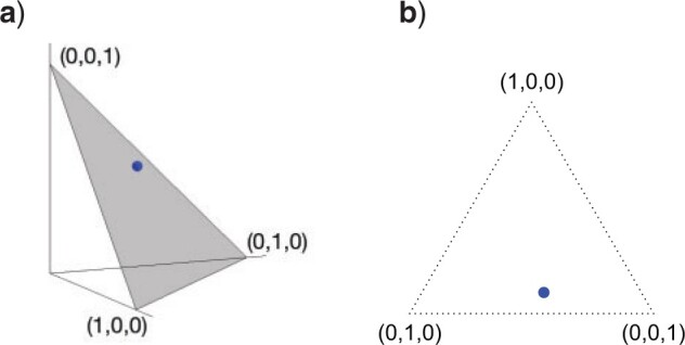
a) The probability simplex in 3D space is a 2D equilateral triangle. Any quartet concordance factor can be viewed as a point in the simplex. b) The simplex, and the concordance factor depicted in it, can be drawn in the plane.

Any quartet concordance factor is represented by a point in this triangle. The vertices represent s where across all gene trees only one quartet topology occurs for the four taxa, the edges of the simplex include those s where only two quartet topologies occur, and interior points those s where all three topologies occur. The centroid is the with equal frequencies of the three topologies.

Note further that if the four taxa are reordered, the entries of the are reordered as well, which gives up to six symmetrically placed points that might represent essentially the same information. For now, we merely insist on having chosen some specific order for each set of four taxa.

Simplex plots of this sort (also called ternary plots) are used in a variety of fields. For example, they can represent color palettes obtained by mixing three primary colors. In phylogenetics, they have been used for purposes other than described here, by Strimmer and von Haeseler (1997) and Smith (2019). Their first published use for representing quartet concordance factors was in several works closely related to this one (Allman et al. 2019b; Baños 2019; Mitchell et al. 2019).

Model Predictions for Concordance Factors

While simplex plots of quartet concordance factors can be made from any collection of gene trees, an interpretation of them hinges on modeling the process by which the trees were generated. Here, we explore expected quartet concordance factors under two models of gene tree generation on a species tree.

Consider first a model for which all gene trees are topologically concordant with the species tree, a model we refer to as the no discord (ND) model. This might also be called the concatenation “supergene” model as it posits that in the absence of any gene tree inference error there is complete gene tree concordance, the only model-based viewpoint which provides justification for noncoalescent concatenation approaches to species tree inference.

Under the ND model, regardless of the choice of four taxa, the expected quartet concordance factor is one of , , or , depending on the arbitrary ordering chosen for the taxa. Thus, a simplex plot of all expected s under the ND model shows points plotted only in the vertices of the simplex, as in Figure 2a. While particular choices of orderings for the different four-taxon subsets might lead to points plotted at only 1 or 2 of the vertices, random orderings typically lead to points at all 3. Regardless, no expected s will appear except at the vertices.

Figure 2.

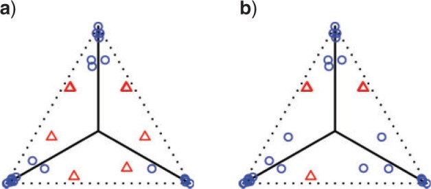
Simplex plots of possible expected for a) the ND and T3 models, b) the MSC and T3 models, c) the ND and T1 models, and d) the MSC and T1 models. For T3, no specific species tree topology is hypothesized. For T1 the model species tree topology is hypothesized.

Now consider the MSC model on a fixed metric species tree . As shown by Allman et al. (2011), depending on taxon ordering the expected for a set of four taxa is one of , , or , with

(1)

where is the length in coalescent units of the internal edge on the species quartet tree for the chosen four taxa. The largest entry, , in the expected indicates the correct topology for the induced quartet species tree. For example, if the tree is displayed on the species tree, then the expected is . Since , in a simplex plot the expected lies on one of the three interior line segments shown in Figure 2b. These line segments extend from the centroid of the simplex, , to the three vertices.

An expected at the centroid arises only when the quartet on the species tree is unresolved, leading to equal probabilities of each of the resolved gene tree quartets. Expected s on the vertical segment arise when the species tree quartet displays the topology , with longer internal edge lengths on the species quartet tree moving the point toward the vertex . That vertex itself corresponds to an infinite edge length, which results in no expected discord between gene trees and the species tree. The other line segments similarly contain expected s for the other two species quartet topologies. Following Mitchell et al. (2019), we refer to the model in which the expected for every quartet lies on the three line segments in Figure 2b as model T3, which stands for “any of 3 possible species quartet trees.” If gene tree production is modeled by the MSC model on any -taxon species tree, regardless of topology or branch lengths, the expected s lie in the model T3.

If the unrooted topology of the metric species tree is hypothesized, then each set of four taxa can be ordered so the first entry of their corresponds to the quartet displayed on . Then under the ND model on the expected for every choice of four taxa will be , lying at the top vertex of the simplex. Under the MSC model on , the expected s all lie on the vertical line from the centroid to the top vertex. Again following Mitchell et al. (2019), we refer to this as model T1, which stands for “1 specific species quartet tree.” Figure 2c,d shows these possibilities graphically.

For a fixed metric species tree on taxa, each of the expected s can be plotted on the same simplex plot. Because under the MSC the expected depends only on the internal branch length of the quartet tree on , some of these points will be the same; the internal quartet branch is determined by its endpoints, which must be two of the internal nodes on an unrooted binary tree. This means there can be only different expected s, up to ordering of the entries. Thus, up to the ordering, there are on average copies of each expected . For a simplex plot made under model T3, these are typically scattered across the model line segments, and some may appear symmetrically located. In a T1 simplex plot made by hypothesizing the model species tree topology, the expected s will all lie on the same vertical line segment. Figure 3 illustrates this for the expected s arising under the MSC for the specific eight-taxon species tree shown in Figure 3a with T3 and T1 simplex plots shown in Figure 3b,c.

Figure 3.

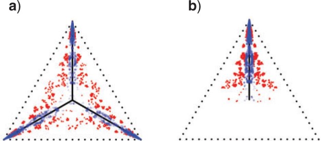
a) An eight-taxon species tree, with branch lengths in coalescent units. b) Expected s under the MSC on this tree in a T3 plot, for which the topology of the species tree is not specified. Expected s appear at a discrete set of points along the three line segments, with some symmetrically located. c) Expected s under the MSC in a T1 plot, when the model species tree topology has been hypothesized. Expected s appear at a discrete set of points on only the vertical line segment. When the thickened edge in the tree of (a) is lengthened by introducing a population bottleneck, expected CFs for quartets whose internal edge includes the lengthened one move toward the vertices in both T3 (d) and T1 (e) plots. In all figures the expected CF represented by a magenta is for the taxa .

It is instructive to modify the tree in Figure 3a to see the effect on expected s. Figure 3d,e shows simplex plots of expected s for such a modified tree, which differs only by the introduction of a population bottleneck on a single edge. As lengths in coalescent units are the number of generations divided by population size, this is modeled by simply increasing that single edge length. Many expected s are left unchanged, because at least three of the four taxa lie on one side of this edge. However, if two of the four taxa lie on each side of the edge, there is an impact on the expected . For a tight bottleneck, essentially all the gene trees will display quartet trees for these taxa that match those of the species tree. The expected s under the MSC then lie close to the vertices of the simplex. Indeed, in Figure 3d,e, we see more expected s close to the simplex vertices than in Figure 3b,c, though some are left unchanged. Note that under the ND model there is no change in the simplex plot when a bottleneck is introduced.

For any model of gene tree generation more general than the MSC, such as one including hybridization, or gene duplication and loss, etc., expected s may not lie on the T3 or T1 model lines. An example of this is given by introducing a single hybridization into the tree of Figure 3a to give the network of Figure 4a. Here there is one hybrid node which has only one descendant taxon, with lineages following one or the other hybrid edge with probabilities 0.3 and 0.7. Because of this simple structure, the gene tree distribution under the Network MSC model is a 30–70% mixture of those that arise under the MSC on the two trees displayed on the network. In the T3 plot of Figure 4b, only expected s under the Network MSC that involve the hybrid taxon are moved from their locations in the plot of Figure 3b, with many s displaced from the model lines. In general, the number of s affected depends on the number of edges in the cycle introduced in the network, the number of descendants of the hybrid node, and other details of the network structure. In contrast, the situation is much simpler for a network ND model, in which every gene tree is displayed on the network. As is shown in Figure 4c, expected s lie either at vertices, or at points on an edge 30% of the way between vertices.

Figure 4.

a) A hybridization network obtained from the tree of Figure 3a by the introduction of an additional edge. With inheritance parameters 0.3 (top hybrid edge) and 0.7 (bottom hybrid edge), T3 simplex plots show expected s under b) the Network MSC and c) a network ND model. Red triangles mark expected s off the model lines, while blue circles mark those on the lines.

Allman et al. (2019b) showed that even if hybridization is limited to that described by networks that are level-1 (i.e., with all cycles disjoint), then an expected under the Network MSC may be located at any point in the simplex. Thus while simplex plots may visually suggest whether the ND or the MSC models might give reasonable fit to a data set, they are not able to immediately suggest which of many more complex biological processes must be modeled to capture important features of some data sets.

Sampling Error and Statistical Tests

If a model allows for gene trees to vary, a finite sample is unlikely to match expectations due to sampling error. However, statistical tests can be developed to measure whether the deviation from expectation is sufficiently large for a given data set to reject the model as a likely explanation of the data. Note that this sampling error is distinct from the gene tree inference error, which arises when the gene trees are inferred from sequence data.

The ND Model

Under the ND model, every gene tree in a sample matches the species tree topology. Thus with probability 1 empirical s for all choices of four taxa must lie at the vertices of the simplex. This is shown in Figure 2a for the model T3, and in Figure 2c for the model T1 if the correct species tree topology is hypothesized. There is no possibility that sampling error causes empirical s to vary from expectation.

A procedure using a as a statistic for testing the ND-T3 model is then trivial. For a fixed choice of four taxa, consider the null and alternative hypotheses:

is then rejected exactly when an empirical lies anywhere other than at a vertex in a T3 simplex plot. For the ND-T1 model the null hypothesis is a specific four-taxon unrooted species tree topology, and the alternative encompasses both other tree topologies and nontree-like evolution. The null is rejected if the T1 simplex plot shows an empirical at any point other than the top vertex. If these tests are applied for all choices of four taxa among a larger set, the ND model on an unknown tree, or more specifically on trees with topology , is rejected if it is rejected for any single choice of four taxa.

Of course such tests have only pedagogical value. In practice, gene trees should not be viewed as sampled from the ND model, but rather from a model with inference error introduced when gene trees are inferred from sequence data. Such an error model would ideally account for impact of sampling error in the sequences (since they are of finite length) as well as any mild model misspecification in the substitution processes used in inference. Use of the ND model hinges on a belief that the observed discord arises solely from such error. Unfortunately, no comprehensive error model has been proposed, and little work has been done to even begin to quantify such error. Without such a model, no more useful test can be developed.

The MSC Model

For the MSC model, in contrast, one can develop useful statistical tests to apply to statistics. Focusing first on the T1 simplex plot, assuming the correct species tree topology is hypothesized, an expected is a point on the vertical line segment shown in Figure 2d. Then a finite sample of gene quartets has quartet counts determined by a random sample from the trinomial distribution with parameters given by the expected . (If an unresolved quartet count has been treated as the noninteger counts (1/3,1/3,1/3), then technically the cannot be viewed as a trinomial sample, but this raises no practical issues.) An empirical computed from a finite sample of gene trees should then be a point near the expected , and by the Law of Large Numbers as the sample size is increased it is increasingly likely to lie close to the expected . Informally, if an empirical is near the vertical line segment it offers support for , while if it is far away it suggests rejection of . However, the size of the sample must be taken into account in giving precise meanings to “near” and “far.”

To formalize these ideas, for four taxa and an unrooted species tree topology consider the null and alternative hypotheses for the MSC-T1 model:

For four chosen taxa, compute the from the gene tree data. Then from the , compute maxima of the likelihood functions under both the null and alternative models in order to find the likelihood ratio statistic for the .

A standard approach, suggested by (Degnan and Rosenberg, 2009), would be to use a distribution with 1 degree of freedom to obtain a value. While this can be justified if the is not near the centroid or a vertex of the simplex, it is problematic near these points. The theoretical argument for the use of the distribution requires the model to be well approximated by its tangent line, and near the boundary point of the T1 model at this is not valid. Near the vertex , which corresponds to a long internal branch on the species tree quartet, we may have very small expected counts of the discordant quartet topologies, and other well-known issues arise with using the when expected counts are low.

When not hypothesizing a specific species tree topology, a test can be performed for the MSC-T3. Again, far from the vertices and the centroid a standard test can be formulated with the likelihood ratio statistic using the distribution with 1 degree of freedom. However, the singularity of the model, where the three lines come together at the centroid, prevents justification of this in its vicinity. The possibility of small expected counts near the vertices also remains problematic.

Better behaved statistical tests for fit of s to the T1 and T3 models, which take into account the boundary or singularity at the centroid as well as small count issues near the vertices, have been developed by Mitchell et al. (2019) and are implemented in the R package MSCquartets (Allman et al. 2019a). While other tests have been developed which can reject a species tree model of evolution, these are the first to account for the full geometry of the model, and, in the case of the T3 test, not to require a specific tree hypothesis. The package enables tabulation of all s for a set of gene trees, computation of values measuring fit to either of the models T1 or T3, and creation of a simplex plot. A small value indicates that it is unlikely a arose under the model, suggesting rejection of the model. There are several options as to the precise test one might use, as discussed more fully in the documentation to the MSCquartets package (Allman et al. 2019a) and by Mitchell et al. (2019). In this article, we adopt the default choices of the function quartetTreeTest in the package, which involves comparison of the statistic to a theoretical distribution in most cases, and an approximation derived from a precomputed bootstrap when expected discordant counts are small. This approximation is very accurate when total counts exceed 30, and allows for fast computations, which is essential when the tests are performed on the large number of s which arise when the number of taxa is large.

Care needs to be taken when using model T1 if the species tree topology is not chosen a priori. If an inferred species tree is specified for the T1 test, gene trees may fit better than they would for the true species tree, leading to a conservative test. In particular, the hypothesis test presented here is not designed to choose among several trees to determine which best fits the data.

Although gene trees in a data set may have many taxa, the tests described so far are performed for a single , for one choice of four taxa, at a time. When performed for each choice of four taxa, this raises issues with multiple comparisons being performed on the same data set (the sample of gene trees). Moreover, the observed gene tree quartets are not independent of one another, and their precise dependence structure has not yet been fully analyzed.

To address the multiple testing problem, one can apply the Holm–Bonferroni method (Holm 1979), which does not require independence of the hypotheses for the tests. Since performing a large number of tests makes it more likely some statistics will be extreme even under the null hypothesis, the method can be viewed as a form of inflation of the values, to reduce the probability of a Type I error (erroneous rejection of the null hypothesis). For a significance level , the Holm–Bonferroni method ensures that the probability of one or more Type 1 errors is at most . The method provides a conservative means of rejecting only a subset of the hypotheses for individual quartets that might otherwise have been rejected. When applied to all s for a collection of gene trees, it thus enables one to pinpoint quartets whose tree-likeness is doubtful for the T3 model, or which significantly deviate from the hypothesized tree for the T1 model. This method is also implemented in MSCquartets.

An important point for interpreting simplex plots and hypothesis test results is the difference between a , the counts of quartet topologies, and its associated empirical , the relative frequencies. Although the test is performed on a and thus includes information on the sample size, a simplex plot shows the empirical and contains no information on sample size. Thus, two s might lead to the same empirical plotted in a simplex, yet produce very different values under the same test, due to their differing sample sizes. If the sample size is small one might obtain a relatively large value, while a much larger sample size would give a small value. In particular, when considering simplex plots of empirical s for different data sets, what should be considered near or far from the model lines depends on the sample size, which is not shown in the plot.

Even within a simplex plot for a single data set, if some taxa are missing from some gene trees then different choices of four taxa may lead to differing sample sizes. Thus a plotted empirical which had a large sample size may be associated to a small value, while another empirical plotted further from the model lines may produce a large value due to a smaller sample size. For a data set with some taxa missing from many gene trees, while other taxa are on most gene trees, this may complicate interpretation of a single simplex plot. However, if there are few missing taxa, or a uniform pattern of missing taxa, the effect will be negligible.

Simulations

To illustrate these ideas, and the impact of gene tree inference error, we give a series of results from simulations, performed using SimPhy (Mallo et al. 2016) for the multispecies coalescent process and Seq-Gen (Rambaut and Grass 1997) for sequence simulation, with gene trees inferred by IQ-TREE (Nguyen et al. 2015). We briefly describe the simulation process here; full details can be found in the Appendix of the Supplementary material available on Dryad at https://doi.org/10.5061/dryad.34tmpg4hq.

We fix a 15-taxon ultrametric species tree with branch lengths in generations. With 15 taxa, there are 1365 s summarizing any gene tree collection. Since under the MSC the prevalence of ILS increases with population size , we consider four sizes, , and , which are held constant across all edges of the tree. The choice of (the minimum allowed by SimPhy) leads to essentially instantaneous coalescence of lineages in a population and thus, up to minuscule error in branch lengths, gives gene trees from the ND model. Adopting a choice of parameters for a GTR model of sequence evolution from an empirical study, we considered conversion factors of for to convert gene tree edge lengths from number of generations to substitution units, a range progressing from low to high levels of mutation. Of these, the central value gives levels of substitution that are moderate, with the more extreme choices useful for bracketing behavior.

For each choice of and we simulated gene trees under the MSC, giving samples of fully resolved gene trees without inference error. We then simulated sequences of length bp along each gene tree, and inferred maximum likelihood gene trees from these sequences, using a setting that caused all inferred edges of length to be contracted to length 0. This gave us samples of gene trees with inference error, which included some polytomies.

We investigate these simulated data sets in several ways. First, in Figure 5, for each value of we plot expected s and empirical s from an MSC gene tree sample without inference error. As the value of is irrelevant for this (other than the fact that our pipeline produced an independent sample of topological trees for each ), we show such plots for only one 1000 tree sample, along with a subsample of 100 trees.

Figure 5.

Row 1 shows expected s for the MSC on the 15-taxon species tree for population sizes , , and . Rows 2 and 3 show empirical s for samples of 100 and 1000 gene trees with the same population sizes, simulated under the MSC by SimPhy. Red triangles denote empirical s for which the hypothesis test with level rejects the T3 model, and thus the MSC on a tree.

For population size the expected CF plot appears to be identical to Figure 2a as the expected level of ILS is graphically imperceptible. Larger values of produce more ILS, hence more discordant gene trees, and thus expected s move closer to the centroid. The bottom two rows of Figure 5 show empirical s from MSC samples of 100 and 1000 gene trees. While close to their expectations, many empirical s lie off the model lines. However, as the number of gene trees is increased, the spread from expectation is reduced. Only MSC sampling error is present in the plots in the bottom two rows, since the gene trees were simulated under the MSC process, and not inferred from sequences. Although we applied the T3 hypothesis test with level to each , there were few rejections, as expected.

Figure 6 shows simplex plots for the 1000 gene trees inferred from simulated sequences, for each value of and , where counts of unresolved quartets are omitted. While similar overall to both the expectation plots and the MSC sample plots of Figure 5, the most significant change due to gene tree inference error is that the inference error resulted in s moving inward from the vertices, toward the centroid. Note that this indicates no substantial topological bias was introduced.

Figure 6.

Empirical s for the MSC on the 15-taxon species tree are shown for 1000 gene trees inferred from simulated sequences data of length 500 bp. Population sizes for rows are from top to bottom , , and , and values of for columns are for . Counts of unresolved gene quartets were omitted in this analysis. Red triangles denote empirical s for which the hypothesis test with level rejects the T3 model, and thus the MSC on a tree.

One important observation from these simulations is that under the ND model, it is possible to simulate data sets and produce a simplex plot that may appear to better match expectations under the MSC model than under the ND model. Indeed, in Figure 6, the differences between the lower left plot for and the upper right plot for are not great, even though the first is the ND model with moderate inference error and the second has substantial ILS. A closer look at the data behind these plots, however, reveals signs of poor quality inferred gene trees. For the upper right plot the mean raw (Hamming) distance between all pairs of sequences for all genes is and with this low level of sequence differences, one should expect gene tree inference error to be high. Indeed, virtually all gene trees are inferred with polytomies. For the lower left figure, the mean raw distance is very high, . Here again we expect high gene tree inference error since the sequences have so few sites in agreement. In this case, we found about one quarter of the trees had polytomies. While counting polytomies does not fully assess inference error, it is one indication that inferred gene trees may be of poor quality. For and all parameter choices on the model tree that led to well-resolved inferred gene trees, the great majority of s were plotted in the vicinity of the vertices.

Additional simulation analyses, including ones investigating the effects of the two possible treatments of unresolved quartets, are given in the Appendix of the Supplementary available on Dryad.

Results

We illustrate the use of the quartet simplex plots and hypothesis tests by examining several empirical data sets. The data sets we discuss have appeared in other publications, and we use gene tree collections previously inferred for those works. Although inference error for these gene trees may have been minimized as much as current methods allow, we nonetheless expect such error is still present.

Yeast

The multilocus yeast data set of (Rokas et al., 2003) was used in an early attempt to infer a species tree from genomic data. Here, we consider a much-analyzed subset of it, with 106 gene trees on 8 taxa, and thus 70 different four-taxon sets. Both the initial analysis, and many subsequent ones, for example (Phillips et al. 2004; Collins et al. 2005; Hedtke et al. 2006; Jayaswal et al. 2014), sought a common tree on which all the loci evolved.

There are some polytomies in the gene trees, and we present an analysis treating unresolved quartets as of each resolution. Results are similar if unresolved quartets are discarded. Figure 7a shows a simplex plot and T3 hypothesis test results for each , using an initial significance level of 0.05. Momentarily ignoring the color/shape-coded hypothesis test results in the figure, a glance at the simplex plot shows some empirical s far from the T3 model lines, suggesting the MSC on a species tree is not consistent with these data. However, with only 106 gene trees, one might at first imagine that the deviations we see from the model lines could be due to chance.

Figure 7.

Simplex plots of empirical s for a Yeast data set of (Rokas et al., 2003), composed of 106 gene trees on 8 taxa. Hypothesis tests results are shown under the T3 model with a) and b) . Red triangles indicate rejection of the null hypothesis and blue circles failure to reject.

The hypothesis tests, however, allow the number of gene trees to be taken into account in interpreting which plotted s are extreme. With a level of , the results of independent tests for each give some red triangles in the plot, further indicating rejection of the MSC on a species tree. However, since these tests are designed to address only sampling error, and gene tree inference error is likely present, a smaller level might be preferred.

A more detailed inspection of values from the T3 test shows the nine empirical s plotted as red triangles closest to the simplex boundary have , while the remaining five plotted as red triangles in Figure 7a have . The next largest value, which is associated to a point plotted as a blue circle, is approximately 0.0894. Lowering the test level to yields the plot of Figure 7b which separates between the two most extreme groups, showing rejection only for one. Varying over several choices allows viewers to visually distinguish levels of model fit. We strongly caution against over reliance on any single threshold as determining which quartets fit the model and which do not. Data sets of gene trees are likely to be somewhat noisy due to inference error, and this may lead to smaller values. Nonetheless, the values provide a standardized way of quantifying “extremeness” across all choices of four taxa.

We apply the Holm–Bonferroni method, with , to adjust for multiple testing without an assumption of independence. This leads to rejection of the null hypothesis for only the nine choices of four taxa giving the smallest P values, whose empirical s are shown as red triangles in Figure 7b. In fact, even though the Holm–Bonferroni adjustment is quite conservative, a level of or smaller would be needed to avoid all rejections of the null hypotheses that the gene trees arose from the MSC on a species tree.

An alternative viewpoint is that all or most of the gene tree discord in this data set is due to gene tree inference error. There is no principled way to rule out that possibility, in part since model misspecification might have played a role when inferring the gene trees. However, general acceptance of the validity of standard phylogenetic methods argues otherwise. It should be emphasized that the methods introduced here use only unrooted topologies of gene trees, which is considered to be the aspect of gene trees that can be most accurately inferred. At the very least, a claim of such extreme inference error should require a detailed argument as to why gene tree error would be so great for certain quartets and not others. Assuming that gene tree inference error is not large, a reasonable conclusion is that this data set is not consistent with the MSC on a species tree, and thus also not consistent with its ND submodel.

With the MSC on a species tree rejected, one might next consider that the taxa should be related by a network. Indeed, many authors (Holland et al. 2004; Wu et al. 2008; Bloomquist and Suchard 2010; Huson et al. 2010; Yu et al. 2011; Zhang et al. 2017; Wen and Nakhleh 2018) have considered a network as appropriate for these data, and investigated evidence for reticulations. Particularly relevant is the recent inference of a network from these gene trees under the Network MSC model by Allman et al. (2019b) using NANUQ. In that algorithm rejection of the T3 model for a leads to use of a hybridization model for the four taxa, and with all hybrid quartets so identified a network can be quickly inferred. In the Appendix of the Supplementary available on Dryad, we present inferred NANUQ networks, and compare their reticulations to those from other statistical analyses.

Mammals

The multilocus mammal data set of Song et al. (2012) was first analyzed under the MSC using both the rooted triple pseudolikelihood algorithm MP-EST (Liu et al., 2010) as well as the clade-based distance algorithm STAR (Liu et al. 2009), to obtain a species tree. The conclusions of those analyses were disputed by Gatesy and Springer (2013), who found fault with using the MSC as a basis for species tree inference in the presence of gene tree inference error, preferring a direct “supergene” analysis of the concatenated sequences. See also the response from Wu et al. (2013).

From the standpoint of model-based inference, this controversy is based on a choice between the ND model of “no discord among true gene trees” and the MSC model of ILS in formation of the gene trees. While hybrid speciation, or any substantial nontree-like signal in the data set, seems unlikely for mammals, we note that both the ND and MSC models simply ignore the possibility.

Since the original collection of gene trees for the data had several errors, we use those from the reanalysis of (Mirarab et al., 2014). This consists of 424 gene trees on 37 taxa, so there are 66,045 choices of four taxa for which the s are tabulated. All gene trees are fully resolved. We explored the data set using a range of testing options, including cutoffs as large as for internal quartet edge lengths to treat quartets as unresolved, and both discarding or redistributing unresolved counts. Here, we present an analysis only for the fully resolved trees, since the other analyses made little difference in conclusions.

The T3 simplex plot on the left in Figure 8a shows that all empirical s for the data set lie relatively close to the model lines. With a level of , which was chosen to accommodate some likely gene tree inference error, the test rejects the MSC on a tree for some quartets. A closer look shows that the smallest values for any choice of four taxa are around , though this arises for points near the simplex vertices, where the most supported topology is clear. Applying the Holm–Bonferroni method, we find no rejection of tree-likeness even for . While this can be a very conservative test, there is no strong evidence for rejecting the MSC on a species tree, a conclusion consistent with other biological knowledge.

Figure 8.

Simplex plots for the Mammal data set of (Song et al., 2012), for 424 gene trees on 37 taxa. In a) model T3 is used, with no specific species tree topology hypothesized. T1 tests use as putative species tree that inferred by b) ASTRAL, ASTRAL-III, and QDC, c) MP-EST, and d) a Bayesian concatenation method. All trees are as reported in Mirarab et al. (2014). See original publications for more complete descriptions. With , red triangles indicate rejection of the null hypothesis, and blue circles failure to reject.

Moreover, the clustering of points in the plot is reminiscent of the equality of expected s for many quartets, as discussed for Figure 3, a feature which in simulation leads to clusters of empirical s. Thus, we find ILS a simpler explanation of this plot than the presence of substantial gene tree error mimicking ILS and suggest a coalescent-based analysis is warranted.

After inferring a species tree topology from the data set by any method one chooses—whether based on the MSC or not—a new simplex plot can be produced hypothesizing the inferred topology for the model T1. For the mammal data, we consider three different choices of hypothesized species trees which have appeared in earlier analyses. The trees are estimated by the coalescent-based ASTRAL and MP-EST, and a noncoalescent-based Bayesian concatenation analysis, as described by (Mirarab et al., 2014) (and, in part, for the original data set by (Song et al., 2012)). We also inferred species trees by the MSC based methods ASTRAL-III (Zhang et al. 2018) and QDC (Rhodes 2020), obtaining the same species tree as from ASTRAL.

The MP-EST tree differs from each of the other two by one nearest neighbor interchange (NNI) move, while the ASTRAL and concatenation tree differ from each other by two NNIs. The three species trees differ from one another only in the placement of the tree shrew (Tupaia belangeri) by an NNI, and of the placement of one clade (composed of Perissodactyla and Carnivora) by an NNI.

In Figure 8b–d, simplex plots are given for the T1 model hypothesizing these species trees. The visual differences between Figure 8b (ASTRAL tree) and Figure 8c (MP-EST tree), are subtle, involving the placement of the two “lobes” of red triangles located near the centroid. In Figure 8b, these are slightly closer to the model line, suggesting a slightly better fit of the ASTRAL tree than the MP-EST tree. However, our plots and tests are not designed to measure fit to a single species tree, but rather the fit of each independently to the induced quartet tree.

The simplex plot in Figure 8d for the concatenation tree shows more interesting differences from those of Figure 8b,c. Although the concatenation tree differs from the MP-EST tree by only an NNI move applied to a single clade, this affects where a relatively large number of empirical s are plotted, in a “ring” around the centroid. While gene trees sampled directly from the MSC on a species tree with a near 0 length branch can lead to a cloud of s around the centroid, a ring does not arise. Thus, plausible conjectures are either this species tree is not correct, or that the gene tree inference procedure led to a bias away from equal occurrences of the three quartet topologies when the true quartet gene trees had nearly equal frequencies.

Investigating individual values for the T1 tests for the three species trees gives additional insight, but no firm conclusions. For all three, the smallest values arose for quartets whose empirical is plotted near the top vertex of the simplex, where the most supported topology is clear. The proportion of quartets for which the hypothesized species tree topology was rejected is shown in Table 1, with these numbers perhaps suggesting a slightly better fit for the ASTRAL tree. However, whether the MP-EST or concatenation tree is rejected more frequently depends on the value of . (Note: Theory does not suggest that the rejection fraction should be close to , since the tests are not of independent hypotheses. Moreover, since we expect some noise in the inferred gene trees, the fraction rejected is likely to be inflated over what we would see with true gene trees.)

Table 1.

For the mammal gene trees, the proportion of s for which the model T1 determined by a hypothesized species tree leads to rejection at the level , rounded to four decimal places.

Species tree
ASTRAL	0.1108	0.0088
MP-EST	0.1109	0.0189
Concatenation	0.1191	0.0132

One might still argue that most of the discord in these gene trees is due to inference error and adopt concatenation as the only justified analysis. We believe that a combination of the MSC and only moderate inference error provides a more parsimonious explanation of the data. However, from the perspective of the quartet simplex plots and hypothesis tests, there is no definitive evidence in favor of one of the three trees over the others. While one might rank them in the order of (b),(c),(d) from “best” to “worst” fit, the differences these methods reveal are quite minor. Indeed, the conservative Holm–Bonferroni method confirms this by failing to reject the MSC on any of these trees at the level .

Fish

Solís-Lemus and Ané (2016) applied their SNaQ software to a data set of 1183 fully resolved gene trees inferred from sequences collected from 24 fish species first presented by (Cui et al., 2013), to infer network relationships. The choice of a network analysis was based on a high level of discord among the gene trees. A simplex plot for the quartets displayed on the gene trees immediately communicates this, as shown in Figure 9a. The smallest values for the T3 tests are around , and the Holm–Bonferroni method with leads to rejection of the null hypothesis for 1815 of 10,626 tests, about . If the null hypothesis is true, we expect at least one false rejection at most of the time. Since the MSC on a tree cannot explain the data, one must conclude there is either a huge amount of gene tree inference error, or some more complicated model such as hybridization is needed for analysis.

Figure 9.

Simplex plots for the Fish data of Cui et al. (2013), composed of 1183 fully resolved gene trees on 24 taxa. In a), no species tree is hypothesized. In b), the putative species tree inferred by ASTRAL-III and QDC, is used for determining placement under the T1 model. With , red triangles indicate rejection of the null hypothesis, and blue circles failure to reject.

In spite of this finding, we applied ASTRAL-III and QDC to the gene trees, obtaining the same inferred tree by both methods. Figure 9b shows a simplex plot for the model T1 with this hypothesized species tree. The plotted points and values still suggest a need for analysis with a more complicated model, such as one capable of inferring a network. Interestingly, though, we see that almost all plotted points are closer to the T1 model line segment than to line segments from other vertices to the centroid. This suggests that there is a “dominant” tree like signal. Since s arising from hybridization on level-1 networks are convex combinations of those on the trees displayed on the network (Solís-Lemus and Ané 2016; Baños 2019), placement of points in the T1 simplex plot as above shows that the inferred tree here would be displayed in the full network.

Drosophila

Martins et al. (2014) investigated a multilocus Drosophila data set of 4591 gene trees, relating 12 subspecies but with taxa missing from some gene trees. These trees include only single-copy gene families (orthologs), though the full data set included additional gene trees with paralogs. These trees were used in the original publication to benchmark a method of tree inference under a model of gene tree discordance allowing for both ILS and gene duplication and loss. In particular, this is a data set believed to have evolved by processes not modeled by the MSC on a tree.

In Figure 10a,b, we show T3 and T1 simplex plots for these gene trees, where the hypothesized (sub-)species tree for the T1 test is that inferred by ASTRAL-III and QDC. While polytomies were present among the gene trees, and this plot was made by redistributing unresolved quartet counts, there are no qualitative changes if those counts are instead discarded. With the tight clustering of points along the model lines, at first one might imagine the data are well described by the MSC, or even (since plotted points are relatively close to the vertices) result from the ND model with gene tree inference error. However, the smallest values for the T3 test are around , and the Holm–Bonferroni method rejects the null hypothesis for some tests even with . When it rejects the null hypothesis for of tests, about of the tests. Thus, a case can be made for processes other than ILS here, under an assumption that gene tree inference error is not substantial.

Figure 10.

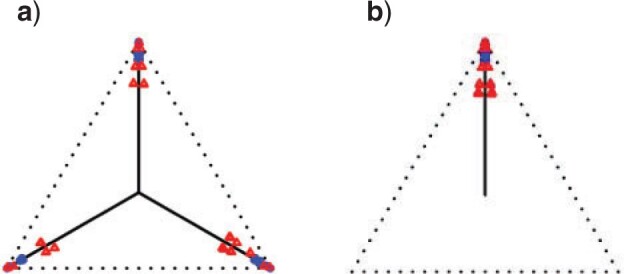
Simplex plots for the Drosophila data of Martins et al. (2014), composed of 4591 gene trees on 12 taxa, with unresolved quartet counts redistributed as resolved. In a), no species tree is hypothesized. In b) the putative species tree obtained by ASTRAL-III and QDC, is used for determining placement under the T1 model. With , red triangles indicate rejection of the null hypothesis, and blue circles failure to reject.

Discussion

Simplex plots of quartet concordance factors offer a concise and easy-to-understand summary of discordance across gene trees. If plotted s fail to cluster along the three T3 model lines, this indicates either substantial gene tree inference error, or the need for analysis with a more complicated model than the MSC, such as one capturing hybridization or gene duplication and loss.

After a species tree is inferred from either gene trees or the original sequence data, by any method a researcher chooses, a new simplex plot under the T1 model hypothesizing the inferred species tree similarly illustrates gene tree discord with that putative species tree. Under the MSC, plotted s should cluster along the T1 model line.

The formal hypothesis tests outlined here can indicate how closely a quartet count concordance factor fits the T1 or T3 model, and rejection of these models implies rejection of the MSC, and its ND submodel, on a species tree. Although these tests fail to account for inference error in gene trees, simulations show that moderate gene tree inference error (in the absence of model misspecification) generally produces no extreme changes in the location of plotted concordance factors away from the model lines, and little change in the distribution of values. In more detail, when gene trees sampled under the MSC are replaced by inferred trees from sequences simulated on them, we graphically notice only a movement of s toward the centroid. Empirical data sets are likely to have additional gene tree inference error from imperfect fit of the substitution model that does cause some spread away from the model lines.

Because of the ubiquitous presence of gene tree inference error, with different gene tree sets possibly having different levels of such error, we caution against using a rigid choice of a level as a meaningful cutoff for rejection for the hypothesis tests. Nonetheless, values are still quite valuable. They offer a measure of model fit for a that can be interpreted relative to others from the same collection of gene trees, all of which can be presumed to reflect similar levels of error. In this way, we can draw meaningful distinctions between those s that may reflect tree-like species relationships under the MSC, and those suggesting more complex processes. With either very high or very low levels of sequence dissimilarity, however, one must be concerned about the quality of the gene tree inference, as even the choice of inference software may affect results.

Under the MSC, the formulas (1) for expected CFs for quartets are very similar to those for expected rooted triple topologies on gene trees. These were given by Pamilo and Nei (1988), and earlier given by Hudson (1983) as approximations under a discrete-time model. Consequently, all of the plots and tests presented here can also be applied to rooted triple counts, which was the setting chosen by (Mitchell et al., 2019). However, when gene trees are obtained from empirical data, rooting is often based on an assumed outgroup. As a result, any incomplete lineage sorting between in- and outgroup taxa may lead to some erroneous rooting, creating an additional source of possible error.

The work of Stenz et al. (2015) is in many aspects close in spirit to what has been presented here, in that it develops tools for measuring fit to a species tree (fully resolved or not) of quartet concordance factors. It differs, however, in the important aspect that it requires a hypothesized metric species tree, while the tests here can be performed without specifying any particular topology (the T3 test), or by specifying a tree topology without branch lengths (the T1 test). In particular, these tests can be especially useful early in an analysis, when it is unclear whether a tree model is even reasonable for the data. Liu et al. (2019) also suggested a hypothesis test, but only for judging which of two metric species trees better fits a gene tree collection, and not for whether the MSC on a species tree should itself be rejected.

An interesting feature of the methods of Stenz et al. (2015) is its use of Dirichlet distributions to model the spread of empirical concordance factors around their “true” values. This can be viewed as a way of modeling unknown noise, so that their estimation of the Dirichlet concentration parameter for a data set might provide some measure of combined sampling and inference error. Whether this approach, or a similar one, can be developed to more explicitly address gene tree error in our framework remains a project for the future.

The hypothesis tests presented here were designed to test the MSC model for a single quartet count concordance factor. While the Holm–Bonferroni method provides one way to apply the test to data for larger trees, it is a conservative approach, giving low power to reject the quartet tree models. This may be acceptable if a researcher is comfortable setting a high bar for suspecting nontree-like species relationships. However development of better testing methods for trees with more than four taxa is certainly needed, though not straightforward. For instance, if several sets of four taxa have the same internal edge in the quartet tree displayed on the species tree, then their expected s are identical, and even with a partial overlap of internal quartet edges they are related. The current tests ignore this fact. Similarly, tests for polytomies on -taxon trees and for individual tree edges under the MSC model are also needed.

With implementations of simplex plotting and hypothesis testing tools in the MSCquartets R package, the methods described here are available for use in both exploring multilocus data sets, and presenting final analyses. In particular, a single simplex plot can communicate much about the level of discord in a collection of gene trees, or of their discord with a hypothesized species tree, allowing readers to form their own judgements of the fit of a data set to an inferred tree. We concur with the statement by Stenz et al. (2015): It “should become standard practice to conduct tests of the population tree model as part of … an analysis.” Although there is still room for improving methodology for such tests, simplex plots of quartet concordance factors provide a very useful beginning.

Supplementary Material

Data available from the Dryad Digital Repository: https://doi.org/10.5061/dryad.34tmpg4hq.

Funding

This research was supported, in part, by the National Institutes of Health Grant (R01 GM117590), awarded under the Joint DMS/NIGMS Initiative to Support Research at the Interface of the Biological and Mathematical Sciences, and 2P20 GM103395, an NIGMS Institutional Development Award (IDeA).

References

- Allman E.S., Degnan J.H., Rhodes J.A. (2011). Identifying the rooted species tree from the distribution of unrooted gene trees under the coalescent. J. Math. Biol. 62(6):833–862. [DOI] [PubMed] [Google Scholar]
- Allman E.S., Baños H., Mitchell J.D., Rhodes J.A. (2019a). MSCquartets: analyzing gene tree quartets under the multi-species coalescent, 2019a. Available from: URL https://CRAN.R-project.org/package=MSCquartets. R package version 1.0.5. [Google Scholar]
- Allman E.S., Baños H., Rhodes J.A. (2019b). NANUQ: A method for inferring species networks from gene trees under the coalescent model. Algorithms Mol. Biol. 14(24):1–25. [DOI] [PMC free article] [PubMed] [Google Scholar]
- Baños H. (2019). Identifying species network features from gene tree quartets under the coalescent model. Bull. Math. Biol. 81(2):494–534. [DOI] [PMC free article] [PubMed] [Google Scholar]
- Bloomquist D., Suchard M. (2010). Unifying vertical and nonvertical evolution: a stochastic ARG-based framework. Syst. Biol. 59:27–41. [DOI] [PMC free article] [PubMed] [Google Scholar]
- Collins T.M., Fedrigo O., Naylor G.J.P. (2005). Choosing the best genes for the job: the case for stationary genes in genome-scale phylogenies. Syst. Biol. 54:493–500. [DOI] [PubMed] [Google Scholar]
- Cui R., Schumer M., Kruesi K., Walter R., Andolfatto P., Rosenthal G. (2013). Phylogenomics reveals extensive reticulate evolution in Xiphophorus fishes. Evolution 67(8):2166–2179. [DOI] [PubMed] [Google Scholar]
- Degnan J.H., Rosenberg N.A. (2009). Gene tree discordance, phylogenetic inference and the multispecies coalescent. Trends Ecol. Evol. 24(6):332–340. [DOI] [PubMed] [Google Scholar]
- Gatesy J., Springer M.S. (2013). Concatenation versus coalescence versus “concatalescence”. Proc. Natl. Acad. Sci. USA 110(13):E1179. [DOI] [PMC free article] [PubMed] [Google Scholar]
- Hedtke S.H., Townsend T.M., Hillis D.M. (2006). Resolution of phylogenetic conflict in large data sets by increased taxon sampling. Syst. Biol. 55:552–529. [DOI] [PubMed] [Google Scholar]
- Holland B.R., Huber K.T., Moulton V., Lockhart P.J. (2004). Using consensus networks to visualize contradictory evidence for species phylogeny. Mol. Biol. Evol. 21(7):1459–1461. [DOI] [PubMed] [Google Scholar]
- Holm S. (1979). A simple sequentially rejective multiple test procedure. Scand. J. Statist. 6(2):65–70. [Google Scholar]
- Hudson R.R. (1983). Testing the constant-rate neutral allele model with protein sequence data. Evolution 37(1):203–217. [DOI] [PubMed] [Google Scholar]
- Huson D.H., Rupp R., Scornavacca C. (2010). Phylogenetic networks. Cambridge: Cambridge University Press. [Google Scholar]
- Jayaswal V., Wong T.K.F., Robinson J., Poladian L., Jermiin L.S. (2014). Mixture models of nucleotide sequence evolution that account for heterogeneity in the substitution process across sites and across lineages. Syst. Biol. 63(5):726–742. [DOI] [PubMed] [Google Scholar]
- Larget B.R., Kotha S.K., Dewey C.N., Ané C. (2010). BUCKy: gene tree/species tree reconciliation with Bayesian concordance analysis. Bioinformatics 26(22):2910–2911. [DOI] [PubMed] [Google Scholar]
- Liu L., Yu L., Pearl D.K., Edwards S.V. (2009). Estimating species phylogenies using coalescence times among sequences. Syst. Biol. 58:468–477. [DOI] [PubMed] [Google Scholar]
- Liu L., Yu L., Edwards S.V. (2010). A maximum pseudo-likelihood approach for estimating species trees under the coalescent model. BMC Evol. Biol. 10(1):302. [DOI] [PMC free article] [PubMed] [Google Scholar]
- Liu L., Anderson C., Pearl D., Edwards S.V. (2019). Modern phylogenomics: building phylogenetic trees using the multispecies coalescent model. In: Anisimova M., editor. Evolutionary genomics. Methods in molecular biology, vol. 1910. New York: Humana. [DOI] [PubMed] [Google Scholar]
- Mallo D., De Oliveira Martins L., Posada D. (2016). SimPhy: phylogenomic simulation of gene, locus, and species trees. Syst. Biol. 65(2):334–344. [DOI] [PMC free article] [PubMed] [Google Scholar]
- De Oliveira Martins L., Mallo D., Posada D. (2014). A Bayesian supertree model for genome-wide species tree reconstruction. Syst. Biol. 65(3):397–416. [DOI] [PMC free article] [PubMed] [Google Scholar]
- Mirarab S., Reaz R., Bayzid M.S., Zimmermann T., Swenson M.S, Warnow T. (2014). ASTRAL: genome-scale coalescent-based species tree estimation. Bioinformatics 30(17):i541–i548. [DOI] [PMC free article] [PubMed] [Google Scholar]
- Mitchell J.D., Allman E.S., Rhodes J.A. (2019). Hypothesis testing near singularities and boundaries. Electron. J. Statist. 13(1):2150–2193. [DOI] [PMC free article] [PubMed] [Google Scholar]
- Nguyen L.-T., Schmidt H.A., von Haeseler A., Minh B.Q. (2015). IQ-TREE: a fast and effective stochastic algorithm for estimating maximum likelihood phylogenies. Mol. Biol. Evol. 32:268–274. [DOI] [PMC free article] [PubMed] [Google Scholar]
- Pamilo P., Nei M. (1988). Relationships between gene trees and species trees. Mol. Biol. Evol. 5(5):568–583. [DOI] [PubMed] [Google Scholar]
- Phillips M.J., Delsuc F., Penny D. (2004). Genome-scale phylogeny and the detection of systematic biases. Mol. Bio. Evol. 21:1455–1458. [DOI] [PubMed] [Google Scholar]
- Rambaut A., Grass N.C. (1997). Seq-Gen: an application for the Monte Carlo simulation of DNA sequence evolution along phylogenetic trees. Bioinformatics 13(3):235–238. [DOI] [PubMed] [Google Scholar]
- Rhodes J.A. (2020). Topological metrizations of trees, and new quartet methods of tree inference. IEEE/ACM Trans. Comput. Biol. Bioinform. 17(6):2107–2118. [DOI] [PMC free article] [PubMed] [Google Scholar]
- Rhodes J.A., Baños H., Mitchell J.D., Allman E.S. (2020). MSCquartets 1.0: quartet methods for species trees and networks under the multispecies coalescent model in R. Bioinformatics 10. doi: 10.1093/bioinformatics/btaa868. [DOI] [PMC free article] [PubMed] [Google Scholar]
- Rokas A., Williams B., Carrol S. (2003). Genome-scale approaches to resolving incongruence in molecular phylogenies. Nature 425:798–804. [DOI] [PubMed] [Google Scholar]
- Sayyari E., Whitfield J.B., Mirarab S. (2018). DiscoVista: interpretable visualizations of gene tree discordance. Mol. Phylogenet. Evol. 122:110–115. [DOI] [PubMed] [Google Scholar]
- Semple C., Steel M. (2005). Phylogenetics. Oxford, UK: Oxford University Press. [Google Scholar]
- Smith M.R. (2019). Bayesian and parsimony approaches reconstruct informative trees from simulated morphological datasets. Biol. Lett. 15(2):20180632. doi: 10.1098/rsbl.2018.0632. [DOI] [PMC free article] [PubMed] [Google Scholar]
- Solís-Lemus C., Ané C. (2016). Inferring phylogenetic networks with maximum pseudolikelihood under incomplete lineage sorting. PLoS Genet. 12(3):e1005896. doi: 10.1371/journal.pgen.1005896. [DOI] [PMC free article] [PubMed] [Google Scholar]
- Song S., Liu L., Edwards S.V., Wu S. (2012). Resolving conflict in eutherian mammal phylogeny using phylogenomics and the multispecies coalescent model. Proc. Natl. Acad. Sci. USA 109(37):14942-14947. [DOI] [PMC free article] [PubMed] [Google Scholar]
- Stenz N.W.M., Larget B., Baum D.A., Ané C. (2015). Exploring tree-like and non-tree-like patterns using genome sequences: an example using the inbreeding plant species Arabidopsis thaliana (l.) heynh. Syst. Biol. 64(5):809–823. [DOI] [PubMed] [Google Scholar]
- Strimmer K., von Haeseler A. (1997). Likelihood-mapping: a simple method to visualize phylogenetic content of a sequence alignment. Proc. Natl. Acad. Sci. USA 94:6815–6819. [DOI] [PMC free article] [PubMed] [Google Scholar]
- Wen D., Nakhleh L. (2018). Coestimating reticulate phylogenies and gene trees from multilocus sequence data. Syst. Biol., 67(3):439–457. [DOI] [PubMed] [Google Scholar]
- Wu Q., James S., Roberts I., Moulton V., Huber K. (2008). Exploring contradictory phylogenetic relationships in yeasts. FEMS Yeast Res. 8:641–650. [DOI] [PubMed] [Google Scholar]
- Wu S., Song S., Liu L., Edwards S.V. (2013). Reply to Gatesy and Springer: the multispecies coalescent model can effectively handle recombination and gene tree heterogeneity. Proc. Natl. Acad. Sci. USA, 110(13):E1180. [DOI] [PMC free article] [PubMed] [Google Scholar]
- Yu Y., Than C., Degnan J.H., Nakhleh L. (2011). Coalescent histories on phylogenetic networks and detection of hybridization despite incomplete lineage sorting. Syst. Biol. 60(2):138–149. [DOI] [PMC free article] [PubMed] [Google Scholar]
- Zhang C., Ogilvie H.A., Drummond A.J., Stadler T. (2017). Bayesian inference of species networks from multilocus sequence data. Mol. Biol. Evol. 35(2):504–517. [DOI] [PMC free article] [PubMed] [Google Scholar]
- Zhang C., Rabiee M., Sayyari E., Mirarab S. (2018). ASTRAL-III: polynomial time species tree reconstruction from partially resolved gene trees. BMC Bioinformatics 19 (Suppl 6)(153):15–30. [DOI] [PMC free article] [PubMed] [Google Scholar]