Predictability of tick-borne encephalitis fluctuations

SUMMARY

Tick-borne encephalitis is a serious arboviral infection with unstable dynamics and profound inter-annual fluctuations in case numbers. A dependable predictive model has been sought since the discovery of the disease. The present study demonstrates that four superimposed cycles, approximately 2·4, 3, 5·4, and 10·4 years long, can account for three-fifths of the variation in the disease fluctuations over central Europe. Using harmonic regression, these cycles can be projected into the future, yielding forecasts of sufficient accuracy for up to 4 years ahead. For the years 2016–2018, this model predicts elevated incidence levels in most parts of the region.

INTRODUCTION

The capacity to understand disease dynamics and predict disease outbursts is the ‘holy grail’ of infectious epidemiology. With tick-borne encephalitis (TBE), a serious Eurasian arboviral infection with a particular reliance on prevention [1], a dependable predictive model has been sought since the discovery of the disease [2–4]. TBE is a classic transmissible zoonosis promoted by an abundance of vectoring ticks and reservoir animals, conditional on but not solely subject to climatic conditions. Most of the proposed models thus regress TBE morbidity against some indicative climatic variables (e.g. mean annual temperature, precipitation) or population estimates of key hosts (e.g. murid rodents) or both. Thanks to a lag in the disease's circulation, 1 year's covariate data can predict the next year's disease incidence. Validity of such a prediction is, of course, contingent on available covariate data and limited to 1–1·5 years ahead.

A possible alternative approach, independent of haphazard environmental data and with a longer projection horizon, is indicated by the finding that TBE fluctuations can be viewed as a superposition of several distinct periodicities that are relatively stable and synchronous over large areas [5]. They can be interpreted as self-oscillations of components of the disease system (such as the populations of ticks, rodents, deer, etc.) that are (secondarily) synchronized/modulated by external (e.g. climatic) factors. In this case, an implicit predictive model would be a harmonic regression fitted to a time series of TBE incidence observed in the past and the present, and extrapolated towards the future.

The aim of the present study is to validate this concept. Based on epidemiological data on TBE in central Europe, an amount of disease variance attributable to plain harmonic oscillations (a (quasi-) biennial, triennial, pentennial, or decadal cycle) is estimated, and the potential to predict future fluctuations is analysed.

METHODS

Epidemiological data

TBE incidence series from Austria, the Czech Republic, Switzerland, and Bavaria (originating from national surveillance systems, and spanning from the early 1970s to 2015) were used in this study. The length of the series is 45 years, except for the Bavarian series, which is 42 years. A previous spectral analysis revealed that there exist cycles of ca. 2·5, 3, 5, and 10 years varying in intensity across central Europe; the four series were chosen to form a representative sample in this respect. The data were de-trended and standardized as described previously [5] to simplify the model and neutralize country-specific effects of population exposure, vaccination, disease reporting, etc.

Model

The harmonic regression model assumes that the incidence series, I, can be expressed in terms of a sum of k sinusoids of fixed amplitude, a, frequency, b, and phase, c, and a superimposed stochastic noise, ε:

where t denotes the time [6]. Based on the previous spectral analysis, k was set to 4 (i = ‘2’, ‘3’, ‘5’, and ‘10’, hereinafter indicates the quasi-biennial, triennial, pentennial, and decadal cycles, respectively), and the noise was assumed to be Gaussian, ε ~ N(0, σ²). The unknown parameters a_2–10, b_2–10, c_2–10, and σ were estimated by means of the Bayesian method, which allowed flexible modifications of the model. All computations were done in the R 3.2.2 software environment interfacing the programme Stan 2.9.0, which is equipped with a fast Markov Chain Monte Carlo computational engine for fitting the model [7]; the R/Stan code is exemplified in the online Supplementary Material.

Prediction

Model predictions were generated using Stan's Monte Carlo built-in facilities (‘generated quantities’ block). To measure the model's accuracy, the means of the predicted distributions of I (year) (taken as point estimates) were set against actual observations, and two common correspondence measures – Pearson correlation coefficient, r, and mean squared deviation, MSD – were calculated. As any predictive model generally performs better within the sample of data that were fitted rather than beyond it, it was also necessary to gain some idea of out-of-sample performance. To this end, a (sliding) segment of 20 observations of an incidence series was used to estimate the parameters of the model, and an ensuing segment of 10 observations served as a diagnostic sample for the forecast. In total, 16 evaluations (14 for Bavaria) were made in a forward direction (each time shifting the subsample windows ahead by 1 year, and re-estimating the prediction accuracy), and analogous 16/14 evaluations were made in a backward direction. All forecast and ‘backcast’ results were combined to assess average prediction accuracy for a decade ahead. To make the model more parsimonious when fitted to the shortened training segments, the frequency parameters (b₂₋₁₀, which consistently showed greatest stability across evaluation trials) were fixed to values obtained from fitting to the full-length series (thus reducing the number of parameters from 13 to 9). Furthermore, assigning greater significance in the regression model to the most recent observations was tested as a means of forecast improvement. This reflects the fact that the disease cycles may evolve over time (e.g. due to climatic changes), and hence their character in an immediately preceding period is more pertinent for their projection into the future than that in the more distant past. For this purpose, the observations were progressively ‘weighted’ along the training segment, forcing the model to fit more closely towards the end of the series. Weights were defined heuristically; the gradient (R = first w/last w; mean w = 1) ranged between 1 and 3.

RESULTS

TBE-fluctuations model

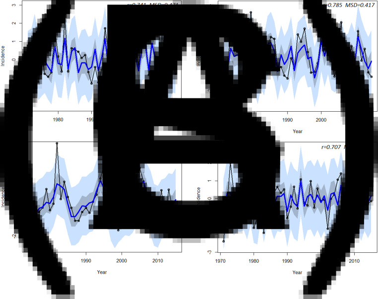
The harmonic regression model fitted to TBE fluctuations is illustrated in Figure 1. The model explains a relatively high proportion of data variance: Pearson's r averages out at ca. 75%, and ranges between 71% and 79% in different regions. The closeness of the fit is obviously conditional on the four oscillations (particularly the 5- and 10-year cycles) being clearly manifest in the disease incidence. The more strongly and uniformly pronounced they are (such as in the Czech Republic), the closer the fit of the harmonic regression. Table 1 summarizes the periods and amplitudes of the cycles as estimated in different regions (further details are shown in online Supplementary Figure S1). While no marked differences are seen between lengths of the periods, the amplitudes are diverse indicating that it is the mixing of the cycles (rather than variability of the cycles themselves) that accounts for the miscellany of regional TBE patterns.

Fig. 1.

TBE incidence (open circles and solid line), and predicted means, 50% and 95% credible intervals (solid line, darker and lighter bands, respectively) from the harmonic regression model: (A) Austria, (B) Bavaria, (C) Czech Republic, and (S) Switzerland.

Table 1.

Oscillations distinguished in TBE fluctuations; shown are periods in years and amplitudes

TBE cycle	Biennial		Triennial		Pentennial		Decadal
	Period (years)	Amplitude	Period (years)	Amplitude	Period (years)	Amplitude	Period (years)	Amplitude
Austria	2·38	0·41	2·94	0·70	5·32	0·19	11·75	0·42
Czech Republic	2·26	0·42	2·95	0·48	5·37	0·51	8·48	0·46
Bavaria	2·40	0·20	2·92	0·20	5·71	0·42	11·42	0·79
Switzerland	2·42	0·49	3·04	0·46	5·33	0·24	9·97	0·24

Prediction accuracy

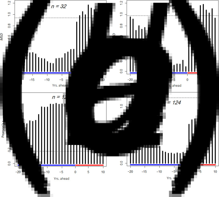
An evaluation of the predictive potential is summarized in Figure 2; it shows that the model can be (with an understandably increasing uncertainty) extrapolated beyond the estimation period. It suggests continuation of the data generating process (i.e., self-oscillations of the disease system) over the background of random turbulent disturbances (e.g. climatic events). The effect of weighting is illustrated in Figure 2a and b; weighting of the regression significantly improves accuracy of the forecast for the next 4 years. In optimized models, the projected and observed incidences are (over the whole validation period) significantly closer to each other than in a null model that assumes independence; the projected and actual data exhibit correlation of ca. 50% over the next 4 years and ca. 40% over the more distant future (Fig. 2c and d).

Fig. 2.

Prediction accuracy of the harmonic regression model: each bar represents n pairs of actual and predicted incidences, dotted lines show thresholds of statistical significance (P = 0·05), and negative and positive values on the time axis correspond to training data and forecast, respectively. Upper panels: comparison of an (a) unweighted and (b) weighted model (R = 3·0) with the Czech data as an example; note that weighting improves accuracy around the end of the training segment including the years +1 to +4. Lower panels: average prediction accuracy across all models expressed in terms of (c) r, and (d) MSD.

Forecast

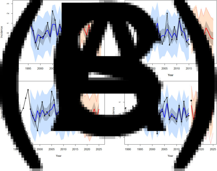
Figure 3 illustrates a TBE forecast for the years from 2016 to 2025. Most importantly, for the next 3–4 years (i.e. within the period of improved accuracy), the model predicts high incidence levels in all areas, with an interim decrease in Switzerland during 2017. A marked increase post-2015 is highly likely in all regions (caused by a culmination of multiple cycles). The probability that TBE levels in Austria, the Czech Republic, Bavaria, and Switzerland will be higher in 2016 than in 2015 can be estimated at 76%, 92%, 84%, and 86%, respectively. Moreover, preliminary epidemiological data available to date for the year 2016 is in close agreement with this forecast (Fig. 3).

Fig. 3.

Harmonic regression model fitted to recent TBE data and projected a decade ahead: actual incidence, predicted means, credible intervals, and the regions are indicated as in Figure 1. Shown is also a naive 95% prediction interval equal to plus or minus twice the root of MSD (dotted lines), and preliminary epidemiological data from the 2016 season (asterisk).

DISCUSSION

This analysis demonstrated that four harmonic oscillations of periods of about 2·4, 3, 5·4, and 10·4 years account for three-fifths of the variation in TBE fluctuations observed across central Europe and make possible their projection into the future. To the author's knowledge, this is currently the only method enabling long-term TBE forecasting. Moreover, it is based solely on routine epidemiological data. There are limitations, however, in making these forecasts.

First, full-scale TBE dynamics combines temporal fluctuations with a long-term trend that was removed from this model. TBE, considered an emerging disease, is increasing in many European countries; however, the trend is far from linear and can be contrasting even in geographically close regions [8]. Implicated drivers range from global warming to socio-economical changes, which add to the perplexity of its prediction. Although it is, in principle, possible to make a statistical forecast using autoregressive methods [9], uncertainty (i.e., a confidence interval) of extension of the trend may exceed that of the fluctuations. Hence, it is pragmatic to keep the trend isolated and forecast only fluctuations on a scale over which the trend is more-or-less unvaried (i.e., ⩽5 years) and update the forecast yearly. This would provide sufficient time for the health system to be adequately prepared.

Second, the model explains the greater part but not all of the variation in TBE fluctuations; when extrapolated beyond the estimation period, more than half of the variation remains unexplained. Both external (e.g. climatic) disturbances and imperfections in the (relatively simple) model may be responsible. For example, the model combines the four cycles additively; however, in nature, co-abundance of ticks with certain hosts has a rather synergetic effect on the extent of disease transmission [10]. This could explain the less successful prediction of the height of some prominent TBE spikes seen in Figure 1. A more elaborate internal structure and inclusion of some external variable(s) might improve the model's performance at least in the short term.

Third, the model relies on the mathematical projection of four oscillations for which the underlying biological mechanisms are not clear. From the lengths of the cycles, it seems they are connected with cycling of the background population levels of ticks and key hosts; a feedback loop between immunity level in a host population and the amount of circulating virus (or similar feedback mechanisms) could also be in play [5]. Any sudden environmental disturbance (in both abiotic and biotic conditions) might shift or interrupt these cycles and invalidate the forecast. Elucidation of the oscillation-generating processes is thus not only a prerequisite for more robust forecasting, but is also needed for understanding of how much a role (by contrast with environmental factors) self-oscillations actually play in the disease dynamics. This is an area for future research.

DECLARATION OF INTEREST

None.

REFERENCES

- 1.Mansfield KL, et al. Tick-borne encephalitis virus – a review of an emerging zoonosis. Journal of General Virology 2009; 90: 1781–1794. [DOI] [PubMed] [Google Scholar]
- 2.Kolman JM. Contribution to the possible forecast of an epidemic of tick-borne encephalitis. In: Rosicky B, Heyberger K, eds. Theoretical Questions of Natural Foci of Diseases. Prague: Publishing House of the Czechoslovak Academy of Sciences, 1965, pp. 209–222. [Google Scholar]
- 3.Naumov RL. On the predictions of tick-borne encephalitis [in Russian]. Parazitologiya 1983; 17: 337–345. [PubMed] [Google Scholar]
- 4.Haemig PD, et al. Forecasting risk of tick-borne encephalitis (TBE): using data from wildlife and climate to predict next year's number of human victims. Scandinavian Journal of Infectious Diseases 2011; 43: 366–372. [DOI] [PubMed] [Google Scholar]
- 5.Zeman P. Cyclic patterns in the central European tick-borne encephalitis incidence series. Epidemiology and Infection 2017; 145: 358–367. [DOI] [PMC free article] [PubMed] [Google Scholar]
- 6.Artis MJ, et al. Harmonic regression models: a comparative review with applications. University of Zurich, Institute for Empirical Research in Economics, Working Paper No. 333, 2007. (http://ssrn.com/abstract=1017519). Accessed 24 October 2016.
- 7.Stan Development Team. Stan modelling language: user's guide and reference manual, Version 2.9.0, 2015 (http://mc-stan.org/documentation). Accessed 15 June 2016.
- 8.Heinz FX, et al. Emergence of tick-borne encephalitis in new endemic areas in Austria: 42 years of surveillance. Eurosurveillance 2015; 20(13): pii=21077. [DOI] [PubMed] [Google Scholar]
- 9.Helfenstein U. The use of transfer-function models, intervention analysis and related time-series methods in epidemiology. International Journal of Epidemiology 1991; 20: 808–815. [DOI] [PubMed] [Google Scholar]
- 10.Randolph SE, et al. Incidence from coincidence: patterns of tick infestations on rodents facilitate transmission of tick-borne encephalitis virus. Parasitology 1999; 118: 177–186. [DOI] [PubMed] [Google Scholar]
Associated Data
This section collects any data citations, data availability statements, or supplementary materials included in this article.
Supplementary Materials
For supplementary material accompanying this paper visit http://dx.doi.org/10.1017/S0950268817001662.
click here to view supplementary material