

Abstract
This article reports spatiotemporal deconvolution methods and simple empirical formulas to correct pressure and beamwidth measurements for spatial averaging across a hydrophone sensitive element. Readers who are uninterested in hydrophone theory may proceed directly to Appendix A for an easy method to estimate spatial averaging correction factors. Hydrophones were modeled as angular spectrum filters. Simulations modeled 9 circular transducers (1–10 MHz; F/1.4–F/3.2) driven at 6 power levels and measured with 8 hydrophones (432 beam/hydrophone combinations). For example, the model predicts that if a 200-μm membrane hydrophone measures a moderately nonlinear 5-MHz beam from an F/1 transducer, spatial-averaging correction factors are 33% (peak compressional pressure or pc), 18% (peak rarefactional pressure or pr), and 18% (full width half maximum or FWHM). Theoretical and experimental estimates of spatial-averaging correction factors agreed to within 5% for linear and moderately nonlinear signals. Criteria for maximum appropriate hydrophone sensitive element size as functions of experimental parameters were derived. Unlike the oft-cited International Electro-technical Commission (IEC) criterion, the new criteria were derived for focusing rather than planar transducers and can accommodate nonlinear signals in addition to linear signals. Responsible reporting of hydrophone-based pressure and beamwidth measurements should always acknowledge spatial averaging considerations.
Keywords: Pressure measurement, hydrophone, deconvolution, beam width, spatial averaging
I. INTRODUCTION
A. Pressure and Beamwidth Measurements
The primary goal of this article and a companion article [1] is to report spatiotemporal deconvolution to correct for effects of hydrophone frequency-dependent sensitivity and finite sensitive element size on pressure and beamwidth measurements. Accurate pressure and beamwidth measurements are essential for documenting experiments and for establishing safety and effectiveness of medical devices.
In this article, a transverse-scan-based spatial deconvolution method is developed and compared with an analytic inverse filter spatial deconvolution method [2–4] that does not require a transverse scan. While both methods predict the effects of spatial averaging on pressure measurements, only the scan-based method predicts the effects of spatial averaging on beamwidth measurements. The analytic inverse filter method is included in IEC 62127–1 Ed. 2 (to be published in 2022).
A second goal of this article is to provide simple empirical formulas to predict dependences of spatial averaging errors in pc, pr, and FWHM on sensitive element size, frequency, F/#, and beam nonlinearity. These formulas can help researchers choose appropriate hydrophones for future measurements or calculate appropriate correction factors for past measurements. These formulas are convenient because they do not require a transverse scan or the considerable signal processing involved for scan-based spatial deconvolution.
Spatiotemporal deconvolution may be divided into two steps: temporal deconvolution and spatial deconvolution.
B. Temporal Deconvolution
The easiest way to convert hydrophone output voltage to acoustic pressure is to divide the voltage waveform by a scalar sensitivity factor (e.g., in units of V/MPa). However, this method is inaccurate when the hydrophone sensitivity varies substantially with frequency across the signal spectrum. In these cases, temporal deconvolution can significantly improve accuracy [5–19].
Temporal deconvolution is particularly helpful for nonlinear signals. Nonlinear signals have significant spectral content at harmonics (integer multiples) of the fundamental frequency due to nonlinear propagation. Harmonic content increases with pressure level and propagation distance [20]. Nonlinear signals are commonly found in acoustic radiation force impulse (ARFI) imaging [21–25], harmonic imaging [26], pulsed Doppler measurements [27], and high intensity therapeutic ultrasound (HITU) [3, 9, 10, 28–31].
C. Spatial Deconvolution
A pioneering approach for spatial deconvolution (a. k. a. “spatial averaging correction”) involved on-axis and off-axis hydrophone measurements that can be used to compute a frequency-independent scale factor for linear pressure waves [32, 33]. Subsequent approaches accommodated linear and nonlinear waves. Some of these employed numerical methods to model spatial averaging [34–38]. Another used an analytic filter [2], which has been validated for membrane, needle, and fiber-optic hydrophones measuring nonlinear signals in diagnostic and HITU pressure ranges [3, 4, 39]. While most spatial averaging correction methods assume circular transducers, one approach has been validated for nonlinear signals transmitted by linear and phased arrays [40–42].
One transverse-scan-based spatial deconvolution method demonstrated improved transverse resolution for narrowband, 2.25-MHz, linear signals detected using receivers with surface areas that were large (63 mm2) compared with most hydrophones (< 0.8 mm2) [43–45]. The method did not consider frequency-dependence of effective receiver size, which has been shown to significantly impact spatial averaging effects for modern hydrophones with geometrical sensitive element diameters of 85–1000 μm [2, 4, 39].
The present article and a companion article [1] report validation of a spatiotemporal deconvolution method for linear and nonlinear signals using transducers (1–10 MHz; F/1–F/3) and hydrophone sensitive element diameters (85–1000 μm) that are relevant to modern ultrasound measurements. The transducers include models designed for HITU.
Fig. 1 illustrates the frequency-dependent relationship between harmonic focal spot size (i.e., FWHM) and hydrophone effective sensitive element diameter deff(f) generated using previously validated models [2, 4, 46]. As harmonic frequency increases, harmonic component beamwidth decreases, thereby increasing the potential for spatial averaging.
Fig. 1.

FWHM at harmonic frequencies for Sonic Concepts H101 transducer (3.3 MHz, F/1) (black asterisks). Also shown are frequency-dependent effective sensitive element diameters deff(f) for five membrane hydrophones with geometrical sensitive element diameters dg of 200 through 1000 μm (dashed lines).
D. Outline of this Article
Section II presents the hydrophone transverse-scan-based spatiotemporal response model and the analytic filter model [2] that will be used for comparison.
Section III describes the simulation, models for hydrophone frequency-dependent effective sensitive element size, and signal processing steps for modeling the hydrophone response.
Section IV shows dependences of spatial averaging errors on hydrophone sensitive element size, frequency, F/#, and nonlinearity.
Section V provides empirical parametric models for spatial averaging corrections for pressure and FWHM as functions of experimental parameters. Formulas are derived for maximum appropriate hydrophone sensitive element size as a function of experimental parameters.
Section VI offers concluding remarks.
Appendix A summarizes a simple method for estimating spatial averaging correction factors.
Appendix B describes a method for quantifying the nonlinearity of a pressure wave.
II. Theory
A. Hydrophone Response Model
For a circularly symmetric transducer, the hydrophone input pressure pulse and the hydrophone output voltage at the measurement plane may be denoted by p(t, r) and u(t, r), where t is time and r is radial distance from the beam propagation axis. Applying spatial and temporal Fourier transformation yields P(f, ρ) and U(f, ρ), where f is temporal frequency and ρ is spatial frequency.
The hydrophone output voltage may be represented in the spatiotemporal transform domain as
| (1) |
ML(f) is the loaded sensitivity of the hydrophone. Dρ[aeff(f), ρ] describes hydrophone directional response, where aeff(f) is the frequency-dependent effective sensitive element radius [46–48].
P(f, ρ) is closely related to the angular spectrum of the incident pressure wave. The difference is that it is expressed as a function of spatial frequency ρ instead of angle θ. Spatial frequency and angle are related by [2, 49]
| (2) |
and may be simplified to ρ = (sin θ)/λ, where λ is wavelength.
Hydrophone directivity is typically expressed as a function of plane-wave incident angle θ. For a circularly symmetric hydrophone, it may be defined as
| (3) |
where k=2π/λ and J1() is a Bessel function of the first kind, order 1. Eq. (3) has been used to model a circular piston in a rigid planar baffle, with aeff(f) set equal to the geometrical sensitive element radius (ag) at all frequencies [50], If aeff(f) is obtained by fitting (3) to frequency-dependent directivity models or measurements, then (3) can be used to accommodate a variety of hydrophone designs. Empirical models for aeff(f) have been obtained for membrane [32, 46, 51, 52], needle [2, 47, 51], and reflectance-type fiber-optic (RTFO) [2, 48] hydrophones.
For spatiotemporal deconvolution, it is convenient to express directivity as a function of ρ.
| (4) |
Spatiotemporal deconvolution may be accomplished using
| (5) |
where U(f, ρ) is the spatiotemporal transform of a transverse scan u(t, r), and Lf (f) and Lρ (f, ρ) are filters to protect from inaccuracies at frequencies where signal-to-noise-ratio (SNR) may be low or either ML(f) or Dρ[aeff(f), ρ] may fall to values far below their maximum levels. Butterworth [3, 4] and Wiener [14] low-pass filters have been used for Lf (f) for sensitivity deconvolution. In the companion article, a Wiener filter is used for Lρ (f, ρ) [1]. Pressure in the spatiotemporal domain, p(t, r), may be recovered by applying inverse temporal and spatial Fourier Transforms to P(f, ρ).
B. Focal Plane Pressure Field (and Spatial Fourier Transform) for a Spherically Focusing Transducer
Since the convolution formula (1) will be tested for circular, spherically focusing piston transducers, it will be useful to derive theoretical forms for the corresponding focal-plane pressure field and spatial Fourier Transform to compare with results obtained numerically (present article) and experimentally (companion article [1]).
The source is assumed to have surface pressure p0, radius as, and radius of curvature R. The transducer is driven at fundamental frequency f1, which corresponds to wavelength λ1 where λ1=c/f1 and c = speed of sound. In the low amplitude limit, in which propagation is linear (i.e., little harmonic generation), the radial pressure distribution for the fundamental component at the focal plane is given by [53]
| (6) |
where k1=2π/λ1 and jinc() is defined by [54]
| (7) |
Eq. (6) is similar in magnitude to the far field diffraction pattern from a circular, planar source [54, 55].
In the present article and the companion article [1], driving voltages are allowed to be sufficiently high to generate significant harmonic activity. However, it has been demonstrated that (6) is still a good approximation for the fundamental component at diagnostic [2, 4, 39] and even high-intensity therapeutic [3] levels. In the present article, the validity of (6) is investigated by evaluating the dependence of the FWHM of the fundamental component of the beam at the focal plane as a function of nonlinearity. (The spatial deconvolution method described in Sec. II-A does not rely on this assumption, however.)
The two-dimensional spatial Fourier transform of a circularly symmetric function is given by the Hankel or Fourier-Bessel transform [54].
| (8) |
where J0() is a Bessel function of the first kind, order 0. In order to take the Hankel transform of (6), it is useful to note that, for typical medical ultrasound pressure waves, the radial variation of the quadratic phase factor, exp[ik1r2/(2R)], is gradual compared with the radial variation of the jinc[asr/(λ1R)] factor, as has been shown previously (see [2], sec. II-E, (18) and (19)). Therefore, the quadratic phase factor may be ignored here.
The Hankel transform of jinc(br) (where b is a scale factor) is [54, 56]
| (9) |
where circ(x) =1 (x< 1); ½ (x=1); 0 (x>1) [54]. Therefore, the magnitude of the spatial Fourier Transform of (6) is approximately given by
| (10) |
Eq. (10) implies that the spatial Fourier Transform has a sharp cutoff spatial frequency at ρcutoff=as/(λ1R). This is tested numerically in the present paper and experimentally in the companion article [1].
C. Analytic Filter Method for Estimating Spatial Averaging
The spatiotemporal deconvolution analysis just presented will be compared with an inverse analytic filter approach that has been validated for membrane, needle, and fiber-optic hydrophones measuring nonlinear signals in diagnostic and HITU pressure ranges [3, 4, 39]. The analytic spatial averaging filter Sp(f) for a nonlinear tone burst is given by [2]
| (11) |
where
| (12) |
f=nf1, n is the harmonic number, and the magnitude of the radial profile of each harmonic component of the nonlinear beam is given by |wn(r)|=exp(−r2/2σn2) for r values extending from 0 to the outer edge of the hydrophone effective sensitive element [2]. Eq. (11) is a low-pass filter that depends on the ratio of the frequency-dependent hydrophone effective sensitive element area to the frequency-dependent beam −6dB area. The fundamental component Gaussian beam width parameter is given by σ1≈1.93R/(k1as) [2]. The harmonic beam width parameters are given by σn=σ1/nq, where q is approximately 0.8 at diagnostic pressure levels (around 5 MPa) [2, 4, 39] and approximately 0.6 at HITU pressure levels (up to 49 MPa) [3]. The FWHM of each harmonic component is [2].
III. Methods
A. KZK Simulation
Simulations used HIFU Simulator Ver 1.2 software [57] to solve the Khokhlov-Zabolotskaya-Kuznetsov (KZK) equation as described previously [2]. Simulation enabled investigation of hydrophone spatial averaging effects over wider ranges of nonlinearity than could be achieved experimentally in the companion article [1]. Experimental pressures are limited by the need to reduce the risk of cavitation and to protect hydrophones from damage. The KZK equation is theoretically valid up to angles of about 15–20° from the propagation axis (approximately equivalent to F/# > 1.5) [58, 59]. The parameters for water used in the simulations were sound speed c=1480 m/s, density ρw=1 g/cm3, absorption at 1 MHz = 0.217 dB/m, exponent of absorption vs. frequency = 2, and nonlinear coefficient β=3.5. One hundred harmonics were used in each simulation. The grid size was 40 points per fundamental wavelength in the axial dimension and 50 points per fundamental wavelength in the radial dimension.
B. Transducers
Table I lists parameters for the single-element, circular, spherically focusing transducers modelled in the simulations. They included Sonic Concepts (Bothell, WA) H151, H196, and H249, which are designed for HITU applications. The other parameters correspond to transducers manufactured by Blatek (State College, PA), and Panametrics (Waltham, MA) (V308, V311 and V381). The driving frequencies (1–10 MHz) and the F/#s (F/1.4–F/3.2) were chosen to encompass a wide range of common applications. Many transducers in Table I were chosen to match transducers for which experimental data were acquired and reported in the companion article [1].
TABLE I.
Transducer Parameters For Simulation
| Manufacturer | Model | Driving Frequency (MHz) | Diameter (mm) | Focal Length (mm) | F/# |
|---|---|---|---|---|---|
| Sonic Concepts | H151 | 1.10 | 64 | 100 | 1.6 |
| Sonic Concepts | H249 | 1.35 | 50 | 125 | 2.5 |
| Sonic Concepts | H151 | 3.41 | 64 | 100 | 1.6 |
| Sonic Concepts | H196 | 3.41 | 40 | 100 | 2.5 |
| Panametrics | V381 | 3.50 | 19 | 38 | 2.0 |
| Blatek | Custom | 3.50 | 64 | 89 | 1.4 |
| Sonic Concepts | H249 | 4.19 | 50 | 125 | 2.5 |
| Panametrics | V308 | 5.00 | 19 | 38 | 2.0 |
| Panametrics | V311 | 10.00 | 12 | 38 | 3.2 |
C. Hydrophones, Sensitivities and Directivities
The first set of simulations assumed membrane hydrophones with nominal geometrical sensitive element diameters of 200, 500, 600, and 1000 μm, corresponding to the four hydrophones used in the companion experimental article [1].
Modeling directivity as a filter requires knowledge of Dρ[aeff(f), ρ] at the frequencies that contribute significantly to the signal (e.g., fundamental and harmonics). Since this set of frequencies might not correspond exactly to the set of frequencies at which directivity was measured, it is useful to have parametric models that can be used to interpolate or extrapolate aeff(f) for any arbitrary set of frequencies.
Frequency-dependent effective sensitive element radii aeff(f) for the membrane hydrophones were derived from directivity measurements at multiple frequencies as described previously [4, 46]. When directivity measurements are unavailable, generic empirical formulas are useful for modeling aeff(f). For membrane hydrophones, an empirical model has been validated: [aeff(f)−ag]/ag=C/(kag)m where ag is the nominal geometrical sensitive element radius, and C and m are fitting parameters, with C=1.89 and m=1.36 [46].
The second set of simulations assumed needle / RTFO hydrophones with nominal geometrical sensitive element diameters of 200, 500, 600, and 1000 μm. For this set, frequency-dependent effective sensitive element radii were predicted using a previously validated “rigid piston” model for needle and RTFO hydrophones [47, 48, 60]. The model gives the effective radius aeff(f) by [aeff(f)−ag]/ag=Aexp(−Bkag), where A=1.85 and B=1.05 [2].
As stated already, another source of distortion for hydrophone measurements of broadband pressure signals is frequency-dependent sensitivity. The effects of frequency-dependent sensitivity have previously been considered and can be countered by inverse filtering [6, 7, 11–13, 17, 18, 61]. The simultaneous effects of frequency-dependent sensitivity and spatial convolution can be managed by applying two separate inverse filters independently, as shown in (5) [4, 42]. To isolate the effects of hydrophone spatial averaging in the simulation, only distortion due to spatial convolution was considered, with the understanding that in practice both forms of distortion occur and can be corrected independently. In the companion article [1], deconvolutions for both frequency-dependent sensitivity and spatial response are performed.
D. Spatial Convolution
The signal model in (1) requires P(f, ρ), which may be computed via spatiotemporal Fourier transformation of the transverse pressure distribution in the focal plane, p(t, r). Therefore, for each source transducer / transmit-power combination, a digitized transverse focal-plane pressure matrix p(jΔt, mΔr) was generated by HIFU Simulator, where Δt was the temporal sampling interval, Δr was the transverse spatial separation between adjacent scan lines, and j and m were integers. Fig. 2 shows an example of a simulated focal waveform.
Fig. 2.

Simulated focal waveform incident upon hydrophone for Sonic Concepts H151 transducer.
The pressure matrix p(jΔt, mΔr) was Fourier transformed along the time dimension using a Fast Fourier Transform (FFT) to yield a spectral pressure matrix P’(jΔf, mΔr) (where the prime denotes that a temporal transform but not a spatial transform has been performed). Fig. 3 shows an example of a focal spectral magnitude. Because of the harmonic structure of the spectra, the spectral matrix could be contracted into a much smaller harmonic matrix PH’(nf1, mΔr) where n is the harmonic number, f1 is the fundamental frequency, and spectral strengths at harmonic frequencies nf1 were found by integrating peaks over frequency intervals nf1±f1/10. Contraction from the spectral matrix P’(jΔf, mΔr) to the harmonic matrix PH’(nf1, mΔr) significantly reduced the number of spatial Fourier transforms required in subsequent steps and therefore significantly reduced computation time. This is consistent with previous models that represented nonlinear pressure signals as sums of harmonics [41, 62, 63].
Fig. 3.

Simulated focal spectral magnitude incident upon hydrophone for Sonic Concepts H151 transducer.
The harmonic matrix PH’(nf1, mΔr) was Hankel transformed along the spatial dimension to give the spatiotemporal transform PH(nf1, sΔρ) where Δρ=ρcutoff/10 was the spatial frequency sampling interval, s was an integer that ranged from 0 to 100 (i.e., ρmax=10ρcutoff) and ρcutoff=as/(λ1R) (see Sec. II-B). (The 2D Fourier transform of a circularly symmetric function is equivalent to a Hankel transform or a Fourier-Bessel transform [64]).
For each transducer / transmit-power / hydrophone combination, UH(nf1, sΔρ) was obtained from (1) by computing the element-by-element product of DρH[aeff(nf1), sΔρ] (for that hydrophone) and PH(nf1, sΔρ) (for that transducer / transmit-power combination). As stated previously, ML(f) was assumed to be one for all frequencies. In other words, it was assumed that in practice spectra would be sensitivity deconvolved independently as has been described previously [4, 6, 7, 11–13, 17, 18, 65].
UH(nf1, sΔρ) was then inverse transformed in the spatial frequency dimension (another Hankel transform), giving UH’(nf1, mΔr), a matrix of transverse beam scans for the fundamental and harmonic frequencies. UH’(nf1, mΔr), could be summed over all harmonic frequencies (the first index) to yield the total broadband, focal-plane, transverse beam scan.
E. Waveform Nonlinearity Indexes
Waveform nonlinearity was characterized by the non-linear propagation parameter 𝜎m [66], local distortion parameter 𝜎q [33, 67], and the spectral index SI [68]. According to IEC 62127–1, 𝜎q < 0.5 corresponds to “little” nonlinear distortion while 𝜎q ≥ 0.5 corresponds to “considerable” nonlinear distortion [33]. SI is the fraction of the power spectrum contained in harmonics of the fundamental frequency [68]. SI, 𝜎m, and 𝜎q have been found to be relatively robust, compared with other nonlinearity metrics, for describing transfer of energy from an ultrasound beam fundamental frequency to higher harmonics [67].
Each simulation was repeated for a range of input powers to generate values of 𝜎q of approximately 0.5, 1, 2, 3, 4, and 5. This corresponded to values of 𝜎m up to approximately 4 and values of SI up to approximately 50%. In addition, all signals could be low-pass filtered to isolate the fundamental signal to simulate linear signals with 𝜎q ≈ 𝜎m ≈ SI ≈ 0.
IV. Results
A. Beam Distortion by Hydrophone in Spatial Domain and Spatial Frequency Domain
Fig. 4 shows simulated focal-plane transverse beam cross sections transmitted by the Blatek transducer and measured with an ideal point hydrophone (dg = 0 μm) and four membrane hydrophones with dg = 200, 500, 600, and 1000 μm. Due to spatial convolution, the measured peak compressional pressure decreases as dg increases.
Fig. 4.
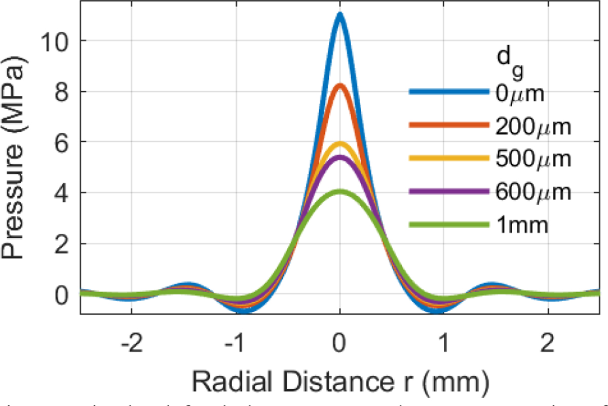
Simulated focal-plane transverse beam cross sections for 3.5 MHz, F/1.4 transducer measured with ideal point hydrophone (dg = 0 μm) and four membrane hydrophones with dg = 200, 500, 600, and 1000 μm.
Fig. 5 shows the first two harmonic components (at frequencies f1 and 2f1) of the spatial Fourier Transform from a simulated transverse scan for the H151 transducer, before and after convolution with the transfer function of the dg=500 μm hydrophone. The simulated spatial Fourier Transform for the fundamental frequency (f1) is close to the theoretically expected function, circ(λ1Rρ/as) from (10). Spatial convolution (i.e., multiplication by directivity in spatial-frequency domain) is a low-pass filter that preferentially passes lower spatial frequency components.
Fig. 5.

Spatial Fourier Transform from transverse scan for the H151 transducer. The first two harmonic components are shown before and after scan-based spatial convolution with the transfer function of the dg=500μm hydrophone. The theoretical function for the fundamental frequency (f1) is circ(λ1Rρ/as) from (10).
B. Effects of Spatial Averaging on Pressure Measurements
Fig.s 6 (membrane hydrophones) and 7 (needle / fiber optic hydrophones) show relative errors due to hydrophone spatial averaging for pc (left column), pr (middle column) and FWHM of pc in the focal plane (right column) as functions of dg/(λ1F/#). The abscissa dg/(λ1F/#) is an index of the ratio of the hydrophone geometrical sensitive element diameter dg to the fundamental component focal spot size. Recall that the FWHM of the fundamental component is 1.41λ1F/# [2, 69]. Linear signals (σq = 0) are shown in top rows of Fig.s 6 and 7, and three levels of nonlinearity (σq > 0) are shown in lower rows.
Fig. 6.

Relative errors due to hydrophone spatial averaging in focal peak compressional pressure pc (left column), focal peak rarefactional pressure pr (middle column) and FWHM (right column) measured with membrane hydrophones plotted as functions of dg/(λ1F/#) for linear signals (top row) and three levels of nonlinearity (other rows). AF-SC: analytic filter spatial convolution. SB-SC: scan-based spatial convolution. See Sec. IV-B.
Fig. 7.

Relative errors due to hydrophone spatial averaging in focal peak compressional pressure pc (left column), focal peak rarefactional pressure pr (middle column) and FWHM (right column) measured with needle / fiber optic hydrophones plotted as functions of dg/(λ1F/#) for linear signals (top row) and three levels of nonlinearity (other rows). AF-SC: analytic filter spatial convolution. SB-SC: scan-based spatial convolution. See Sec. IV-B.
Relative errors in focal pressure magnitudes were computed as (p’−p)/p (where p’ = the measured value subjected to spatial averaging and p = the true axial value that would be obtained with a hypothetical point hydrophone).
Pressure data were modeled using exponential functions, p’/p = exp(−αx), and Gaussian functions, p’/p = exp(−βx2), where x=dg/(λ1F/#). In each case, the model with the lower root-mean-squared difference (RMSD) between simulated data and functional fit was chosen (see Sec. V-B).
Figs. 6 and 7 show excellent agreement between analytic filter spatial convolution (AF-SC) and scan-based spatial convolution (SB-SC), suggesting approximate equivalence of the two methods.
Fig. 8 shows the pressure error parameter αc for pc for membrane hydrophones, computed by AF-SC and SB-SC, as functions of local distortion parameter σq. The AF-SC and SB-SC methods exhibit excellent agreement, reinforcing the validity of both methods. The dependence of αc on σq is linear up to σq = 5. The data are consistent with experimental measurements at σq = 0 and σq = 1 taken from the companion article [1].
Fig. 8.

Relative error parameters αc for focal peak compressional pressure magnitude. σq: nonlinear distortion parameter. SIM: simulation. EXPT: experiment. AF-SC: analytic filter spatial convolution. SB-SC: scan-based spatial convolution. M: membrane hydrophone.
Table II shows data from Fig. 8 with values for σq, σm and SI. Table II also shows previously reported values for the pressure error parameter αc for pc simulated using the AF-SC method for membrane hydrophones [4]. The present and previous values for αc are similar even though the two simulations assumed different sets of source transducers. Table II also shows experimental values from the companion article [1]. For experimental data, ground truth pressure values were estimated from measurements performed with a high-resolution hydrophone (dg=85 μm) that had been corrected using spatiotemporal deconvolution [1].
TABLE II.
Pressure Error Parameter Alpha For Membrane Hydrophones
| Pressure | Compressional | Rarefactional | |||||||||
|---|---|---|---|---|---|---|---|---|---|---|---|
| Data | Simulation | Simulation | Previous Simulation | Expt | Simulation | Simulation | Previous Simulation | Expt | |||
| Method | AF-SC | SB-SC | AF-SC | AF-SC | SB-SC | AF-SC | |||||
| Linearity | σq | σm | SI | αc (RMSD) | αc (RMSD) | αc (RMSD) | αc (RMSD) | αr (RMSD) | αr (RMSD) | αr (RMSD) | αr (RMSD) |
| Linear | 0 | 0 | 0 | 0.24 (3%) | 0.25 (4%) | 0.29 (7%) | 0.24 (3%) | 0.25 (4%) | 0.30 (7%) | ||
| Nonlinear | 0.5 | 0.4 | 4% | 0.31 (3%) | 0.33 (4%) | 0.34 (4%) | 0.20 (3%) | 0.22 (3%) | 0.25 (4%) | ||
| Nonlinear | 1.0 | 0.8 | 12% | 0.40 (3%) | 0.43 (4%) | 0.43 (4%) | 0.40 (8%) | 0.20 (3%) | 0.21 (4%) | 0.23 (4%) | 0.29 (6%) |
| Nonlinear | 2.0 | 1.6 | 29% | 0.65 (5%) | 0.65 (5%) | 0.68 (5%) | 0.20 (3%) | 0.21 (4%) | 0.23 (4%) | ||
| Nonlinear | 3.0 | 2.2 | 35% | 0.76 (4%) | 0.72 (5%) | 0.20 (3%) | 0.23 (5%) | ||||
| Nonlinear | 4.0 | 3.1 | 45% | 0.87 (4%) | 0.84 (5%) | 0.19 (3%) | 0.24 (5%) | ||||
| Nonlinear | 5.0 | 3.9 | 49% | 0.95 (4%) | 1.01 (4%) | 1.02 (5%) | 0.18 (3%) | 0.23 (3%) | 0.23 (4%) | ||
Exponentially decaying model functions, exp(-αx), were fit to focal pressure magnitude ratios p’/p (where p’ = measured value subjected to spatial averaging and p = true axial value that would be obtained with a hypothetical point hydrophone), where x = dg / (λ1F/#). Nonlinearity indexes are σq (local distortion parameter), σm (nonlinear propagation parameter), and SI (spectral index). RMSD: root-mean-squared difference between data and functional fits. AF-SC: analytic filter spatial convolution. SB-SC: scan-based spatial convolution. Previous simulation data are from Wear et al., IEEE Trans. Ultrason. Ferro., Freq. Control., 67(12), 2674–2691, 2020.
Fig. 9 shows the pressure error parameter αr for pr for membrane hydrophones, computed with both AF-SC and SB-SC methods, as functions of local distortion parameter σq. The AF-SC and SB-SC methods exhibit excellent agreement, reinforcing the validity of both methods. The parameter αr is nearly independent of σq up to σq = 5. This is because, as can be seen in Fig. 2, increases in harmonic content due to increases in σq are manifested more in the compressional component (which varies rapidly with time) and less in the rarefactional component (which varies slowly with time) [70]. The data are consistent with experimental measurements at σq = 0 and σq = 1 taken from the companion article [1]. By comparing Figs. 8 and 9, it may be seen that at σq = 0, αc ≈ αr. This is because at σq = 0, the wave is linear and therefore pc ≈ pr.
Fig. 9.

Relative error parameters αr for focal peak rarefactional pressure magnitude. σq: nonlinear distortion parameter. SIM: simulation. EXPT: experiment. AF-SC: analytic filter spatial convolution. SB-SC: scan-based spatial convolution. M: membrane hydrophone.
Fig.s 10 and 11 (and Table III) are like Figs. 8 and 9 (and Table II), except that they were generated assuming needle / RTFO hydrophones instead of membrane hydrophones. Similar trends are apparent.
Fig. 10.
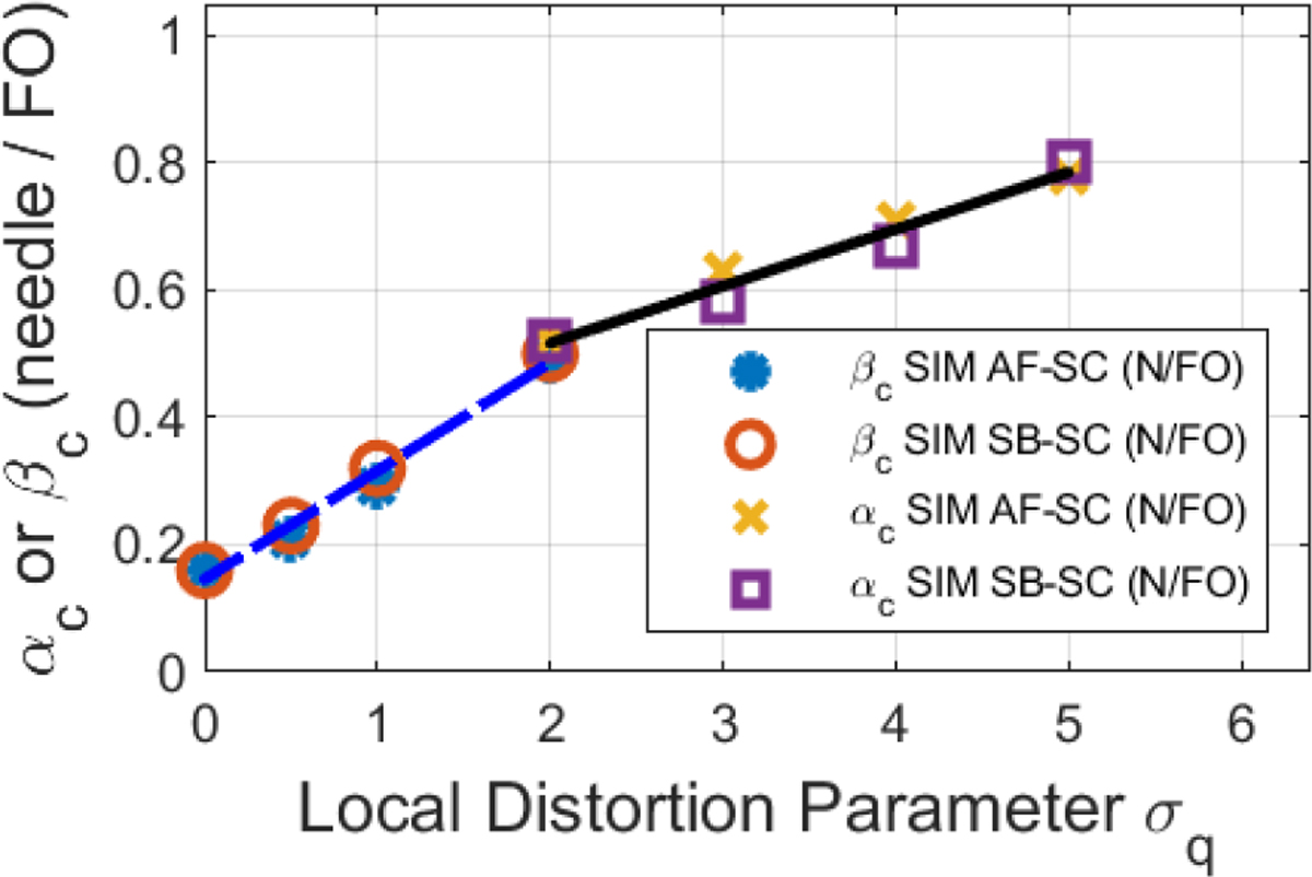
Relative error parameters αc and βc for focal peak compressional pressure magnitude. σq: nonlinear distortion parameter. SIM: simulation. AF-SC: analytic filter spatial convolution. SB-SC: scan-based spatial convolution. N/FO: needle or RTFO hydrophone.
Fig. 11.

Relative error parameters βr for focal peak rarefactional pressure magnitude. σq: nonlinear distortion parameter. SIM: simulation. AF-SC: analytic filter spatial convolution. SB-SC: scan-based spatial convolution. N/FO: needle or RTFO hydrophone.
TABLE III.
Pressure Error Parameters Alpha and Beta For Needle Hydrophones
| Pressure | Compressional | Rarefactional | |||||||
|---|---|---|---|---|---|---|---|---|---|
| Data | Simulation | Simulation | Previous Simulation | Simulation | Simulation | Previous Simulation | |||
| Method | AF-SC | SB-SC | AF-SC | AF-SC | SB-SC | AF-SC | |||
| Linearity | σq | σm | SI | βc (RMSD) | βc (RMSD) | βc (RMSD) | βr (RMSD) | βr (RMSD) | βr (RMSD) |
| Linear | 0 | 0 | 0 | 0.16 (1%) | 0.16 (1%) | 0.16 (1%) | 0.16 (1%) | ||
| Nonlinear | 0.5 | 0.4 | 4% | 0.21 (2%) | 0.23 (1%) | 0.24 (3%) | 0.13 (1%) | 0.14 (1%) | 0.13 (1%) |
| Nonlinear | 1.0 | 0.8 | 12% | 0.29 (4%) | 0.32 (3%) | 0.30 (5%) | 0.12 (1%) | 0.13 (1%) | 0.13 (1%) |
| αc (RMSD) | αc (RMSD) | βr (RMSD) | βr (RMSD) | ||||||
| Nonlinear | 2.0 | 1.6 | 29% | 0.52 (4%) | 0.52 (5%) | 0.12 (1%) | 0.13 (1%) | 0.12 (1%) | |
| Nonlinear | 3.0 | 2.2 | 35% | 0.63 (3%) | 0.58 (7%) | 0.12 (1%) | 0.15 (3%) | ||
| Nonlinear | 4.0 | 3.1 | 45% | 0.71 (2%) | 0.67 (6%) | 0.12 (1%) | 0.16 (4%) | ||
| Nonlinear | 5.0 | 3.9 | 49% | 0.78 (2%) | 0.80 (6%) | 0.12 (1%) | 0.15 (3%) | 0.13 (2%) | |
Exponentially decaying and Gaussian model functions, exp(-αx) (pc for σq ≥2) or exp(-βx2) (all other pressures), were fit to focal pressure magnitude ratios p’/p (where p’ = measured value subjected to spatial averaging and p = true axial value that would be obtained with a hypothetical point hydrophone), where x = dg / (λ1F/#). Nonlinearity indexes are σq (local distortion parameter), σm (nonlinear propagation parameter), and SI (spectral index). RMSD: root-mean-squared difference between data and functional fits. AF-SC: analytic filter spatial convolution. SB-SC: scan-based spatial convolution. Previous simulation data are from Wear et al., IEEE Trans. Ultrason. Ferro., Freq. Control., 67(12), 2674–2691, 2020.
C. Effects of Spatial Averaging on FWHM Measurements
Relative errors in FWHM were modeled using linear model functions, FWHM’ / FWHM = 1 + Cx. Fig. 12 shows the FWHM error parameter C for membrane and needle / RTFO hydrophones, computed with SB-SC, as functions of local distortion parameter σq. The dependence of C on σq is linear up to σq = 5 for both types of hydrophones. The values of C for membrane hydrophones are very consistent with experimentally-derived values taken from the companion article [1].
Fig. 12.

Error parameter C for FWHM as a function of nonlinear distortion parameter σq. SIM: simulation. SB-SC: scan-based spatial convolution. EXPT: experiment. M: membrane hydrophone. N/FO: needle or RTFO hydrophone.
Table IV shows the data from Fig. 12 in numerical form. Table IV also includes values for σm and SI.
TABLE IV.
FWHM Error Parameter C For Membrane and Needle Hydrophones
| Hydrophone Type | Membrane | Membrane | Needle | |||
|---|---|---|---|---|---|---|
| Data | Simulation | Expt | Simulation | |||
| Method | SB-SC | SB-SC | SB-SC | |||
| σq | σm | SI | C (RMSD) | C (RMSD) | C (RMSD) | |
| Linear | 0 | 0 | 0 | 5% (2%) | 9% (4%) | 4% (3%) |
| Nonlinear | 0.5 | 0.4 | 4% | 16% (4%) | 14% (5%) | |
| Nonlinear | 1.0 | 0.8 | 12% | 30% (5%) | 30% (10%) | 27% (6%) |
| Nonlinear | 2.0 | 1.6 | 29% | 62% (9%) | 57% (10%) | |
| Nonlinear | 3.0 | 2.2 | 35% | 74% (10%) | 67% (12%) | |
| Nonlinear | 4.0 | 3.1 | 45% | 100% (13%) | 89% (14%) | |
| Nonlinear | 5.0 | 3.9 | 49% | 120% (20%) | 109% (20%) | |
Linear model functions Cx were used to fit to relative errors in FWHM, where x = dg / (λ1F/#). Nonlinearity indexes are σq (local distortion parameter), σm (nonlinear propagation parameter), and SI (spectral index). RMSD: root-mean-squared difference between data and functional fits. SB-SC: scan-based spatial convolution.
V. Discussion
A. Comparison of Two Spatial Averaging Models
Two methods (AF-SC and SB-SC) were compared for modeling the effects of hydrophone spatial averaging on pressure measurements for linear and nonlinear signals. The AF method has the advantage that it can be performed on axial pressure measurements, without the need for a transverse scan. The analytic filter (11) can be computed based on transducer and hydrophone properties. Spatial averaging effects may be suppressed by inverse filtering the hydrophone output with the analytic filter. Although the SB method requires a transverse scan, it has the advantage that it can also assess the effects of spatial averaging on beam FWHM.
The analytic filter method makes assumptions about the signal. First, it models the beam as a superposition of gaussian beams with radial profile magnitudes of harmonic components given by |wn(r)|=exp(−r2/2σn2) for r values extending from 0 to the outer edge of the hydrophone effective sensitive element [2]. This approximation has been validated for needle, membrane, and fiber-optic hydrophones at diagnostic and HITU pressure levels [3, 4, 39]. It is validated again in the companion article [1].
Second, the analytic filter model assumes that the FWHM of the fundamental component equals the linear-propagation value. Fig. 13 shows simulated FWHM of the fundamental component as a function of σq for nine simulated source transducers. The theoretical FWHM (1.41λ1F/#) are shown by the horizontal lines. For σq ≤ 6, the fundamental FWHM is approximately equal to the linear-propagation value, even though σq = 6 corresponds to significant nonlinearity. For example, HITU signals at frequencies of 1.5–4 MHz and pressure levels of 16–49 MPa have been reported to have σq values ranging from 3 to 4 [3].
Fig. 13.

Simulated FWHM of fundamental component as a function of nonlinear distortion parameter σq for nine transducers. The theoretical FWHM is 1.41 λ1 F/#.
Based on the simulation results of the present article and the experimental results of the companion article [1], the two methods give very similar results for pressure measurements performed using membrane, needle, and RTFO hydrophones at frequencies ranging from 1–10 MHz, F/# ranging from 1.4–3.2, and nonlinear distortion ranging from none (σq = 0) to severe (σq = 5), as shown in Figs. 6 and 7, and Tables II and III.
B. Simple Empirical Formulas to Correct for Finite-Sensitive-Element Effects
Figs. 6 and 7 show that spatial averaging errors are largely determined by a small set of experimental parameters: hydrophone type, dg, λ1, F/#, and σq. (Of these, the only one that requires some effort to estimate is σq—see Appendix B.) Therefore, simple empirical formulas obtained from the analysis presented here may be used to estimate spatial averaging errors when the experimenter knows these parameters.
The best models (lowest RMSD between model and simulation) between measured pressures p’ and spatial-averaging-corrected pressures p were as follows. For membrane hydrophones (σq ≤ 5) and needle / RTFO hydrophones (2 ≤ σq ≤ 5),
| (13) |
where x=dg/(λ1F/#). For needle / RTFO hydrophones (σq ≤ 2),
| (14) |
For membrane hydrophones (σq ≤ 5),
| (15) |
For needle / RTFO hydrophones (σq ≤ 5),
| (16) |
Expressions for αc, αr, βc, and βr may be found in Table V.
TABLE V.
Best Models for Spatial Averaging Errors
| Hydrophone | Parameter | σq range | model | RMSD |
|---|---|---|---|---|
| Membrane | p c | σq ≤ 5 | αc≈0.27+0.15σq | 0.04 |
| Membrane | p r | σq ≤ 5 | αr≈0.24 | 0.03 |
| Membrane | C | σq ≤ 5 | C≈(5+27σq) % | 6% |
| Needle / fiber optic | p c | 0 ≤ σq ≤ 2 | βc≈0.15+0.17σq | 0.01 |
| Needle / fiber optic | p c | 2 ≤ σq ≤ 5 | αc≈0.34+0.09σq | 0.02 |
| Needle / fiber optic | p r | σq ≤ 5 | βr≈0.14 | 0.02 |
| Needle / fiber optic | C | σq ≤ 5 | C≈(3+23σq) % | 5% |
Exponentially decaying and Gaussian model functions, exp(-αx) or exp(-βx2), were fit to focal pressure magnitude ratios p’/p (where p’ = measured value subjected to spatial averaging and p = true axial value that would be obtained with a hypothetical point hydrophone), where x = dg / (λ1F/#). Linear model functions Cx were used to fit to relative errors in FWHM. The local distortion parameter is σq. RMSD: root-mean-squared difference between data and functional fits.
For all hydrophones,
| (17) |
Figs. 8–12 and Table V show the dependences of α, β, and C on σq.
C. Criteria for Maximum Hydrophone Sensitive Element Size when Spatiotemporal Deconvolution is not Performed
To choose an appropriate hydrophone for a measurement, the relative error models may be used to solve for criteria for maximum appropriate hydrophone sensitive element diameters as functions of experimental parameters for cases when spatiotemporal deconvolution is not performed. The relative errors in pressures and FWHM are given by
| (18) |
| (19) |
where, as shown in Table V, α, and β assume different values for compressional and rarefactional pressures, and x=dg/(λ1F/#). First, maximum acceptable relative error levels, εp and εFWHM may be chosen (e.g., −0.1 and 0.1 respectively, corresponding to −10% and 10%). For pressure parameters with exponential spatial averaging error functions,
| (20) |
For pressure parameters with Gaussian spatial averaging error functions,
| (21) |
For FWHM,
| (22) |
where formulas for α, β, and C are given in Table V.
These criteria have advantages compared with a hydrophone maximum sensitive element size criterion from IEC 62127–1 [33, 71]. First, unlike the IEC criterion, (20)–(22) were derived based on focused transducers instead of planar transducers. Although IEC 62127–1 states that its criterion can also be used for focused transducers, it is not optimal for focused transducers since it was derived for planar transducers. Second, unlike the IEC criterion, (20)–(22) allow for nonlinear ultrasound and therefore can accommodate nonlinear modes such as pulsed Doppler, harmonic imaging, ARFI and HITU. (To be fair, nonlinear ultrasound is far more common today than it was in 1985, when the IEC criterion was derived.) Third, unlike the IEC criterion, (20)–(22) provide separate criteria for pc, pr, and FWHM, which allows the investigator to tailor the criterion to a particular measurement task. For example, if cavitation probability is the main concern, then pr is the main parameter of interest. Fourth, (20) – (22) are expressed in terms of the geometrical sensitive element diameter dg, which is often more readily accessible than the effective sensitive element diameter deff (on which the IEC criterion is based).
VI. Conclusion
Two methods have been shown to be equivalent for predicting errors in pressure measurements due to hydrophone spatial averaging over a broad range of experimental parameters: an analytic filter method and a scan-based method. The analytic filter method has the advantage of not requiring a transverse scan. The scan-based method has the advantage of predicting errors in beam FWHM in addition to predicting errors in pressures.
The analysis shows that hydrophone spatial averaging errors can be significant for many common ultrasound experiments. For example, for an F/1 transducer transmitting a moderately nonlinear beam (σq ≈ 1) at 5 MHz and measured with a 200-μm membrane hydrophone, correction factors for peak compressional pressure, peak rarefactional pressure, and FWHM are 33%, 18%, and 18% respectively.
Simple empirical formulas have been obtained for prediction of spatial averaging errors in pressure and FWHM as functions of experimental parameters. Criteria for maximum acceptable hydrophone sensitive element size as functions of experimental parameters have been derived. These criteria are useful for informing choice of an appropriate hydrophone for future experiments.
Using the spatial averaging correction formulas, accurate measurements of focal pressures and FWHM are possible even when the hydrophone geometrical sensitive element diameter exceeds the beam fundamental component focal spot size. This provides investigators with increased flexibility of hydrophone choice, which can be beneficial when selection of hydrophones in a laboratory is limited or when larger sensitive element size is desired for increased sensitivity and increased SNR.
Responsible reporting of hydrophone-based pressure measurements should always acknowledge spatial averaging considerations.
Acknowledgement
The mention of commercial products, their sources, or their use in connection with material reported herein is not to be construed as either an actual or implied endorsement of such products by the Department of Health and Human Services. The authors are grateful for funding support from the FDA Office of Women’s Health.
This article was submitted on Sept. 14, 2021. This work was supported by the U.S. Food and Drug Administration Office of Women’s Health.
Biography
Keith A. Wear (Senior Member, IEEE) received the B.A. degree in applied physics from the University of California at San Diego, San Diego, CA, USA, and the M.S. and Ph.D. degrees in applied physics, with a Ph.D. minor in electrical engineering, from Stanford University, Stanford, CA.
He was a Postdoctoral Research Fellow with Physics Department, Washington University, St. Louis, MO, USA. He is currently a Research Physicist with the U.S. Food and Drug Administration, Silver Spring, MD, USA.
Dr. Wear is a Fellow of the Acoustical Society of America, the American Institute for Medical and Biological Engineering, and the American Institute of Ultrasound in Medicine (AIUM). He received the 2019 AIUM Joseph H. Holmes Basic Science Pioneer Award. He served as Associate Editor-in-Chief for IEEE TRANSACTIONS ON ULTRASONICS, FERROELECTRICS, AND FREQUENCY CONTROL (IEEE-TUFFC) (2019–2021). He has served as Associate Editor of IEEE-TUFFC (2002–2021), Journal of the Acoustical Society of America (2012-present), and Ultrasonic Imaging (2013-present). He was the Technical Program Chair of the 2008 IEEE International Ultrasonics Symposium (IUS), Beijing, China. He was the General Program Chair of the 2017 IEEE IUS, Washington, DC, USA. He has served as chair of the AIUM Technical Standards Committee (2014–2016), AIUM Bioeffects Committee (2021–2023), AIUM Basic Science and Instrumentation Community (2004–2006 and 2014–2016), and AIUM Therapeutic Ultrasound Community (2013–2015). He is Chair of the American Association of Physicists in Medicine Task Group 333 on Magnetic Resonance Guided Focused Ultrasound Quality Assurance. His research interests include hydrophone measurement methodology, high intensity therapeutic ultrasound, photoacoustics, and quantitative ultrasound.
Appendix A: Simple Method for Estimating Spatial Averaging Correction Factors
First, compute x=dg/(λ1F/#) from the hydrophone geometrical sensitive element diameter dg, fundamental wavelength λ1, and transducer f-number F/#.
Second, for nonlinear signals, if x ≤1, use (B5) or (B6) from Appendix B to estimate the local distortion parameter σq from focal pressure measurements pc’ and pr’. (If x > 1, see Appendix B.) For linear signals (e.g., pc ≈ pr), σq ≈ 0. (Note that correction factors for pr’ do not require estimates of σq.)
Third, use formulas in Table V to compute αc or βc, αr or βr, and C.
Fourth, use (13)–(17) to compute spatial-averaging correction factors to convert measured values pc,’ pr’, and FWHM’ into spatial-averaging corrected values pc, pr, and FWHM.
Alternatively, radiofrequency data may be inverse filtered with the analytic filter (11) described in Sec. II-C. If measurements for aeff(f) for the hydrophone (e.g., derived from directivity measurements) are unavailable, then generic versions for aeff(f) given in Sec. III-C may be used. The inverse analytic filter (IAF) method corrects pressure (but not FWHM) measurements for spatial averaging. The IAF method is included in IEC 62127–1 Ed. 2 (to be published in 2022).
This methodology may also be relevant to capsule hydrophones. There is anecdotal evidence that aeff(f) is asymptotically (kag > 0.7) similar for capsule and needle hydrophones (see Fig. 2 in [42]).
Appendix B: How to Estimate σq from Focal Pressure Measurements
The models in Table V for pc and FWHM (but not the models for pr) require knowledge of the local distortion parameter, σq [33, 66, 67, 72],
| (B1) |
where z is the axial propagation distance, pm=(pc+pr)/2, fawf is the acoustic working frequency (fawf ≈ f1), β is the nonlinearity parameter (β=1+B/2A=3.5 for pure water at 20°C), ρw is the density of water (997 kg/m3), Fa is the local area factor,
| (B2) |
ASAeff is the effective source aperture area, and Ab,−6dB is the beam area included within the half maximum pressure contour. ASAeff may be estimated from nominal aperture dimensions or by fitting a theoretical diffraction pattern to a spatially deconvolved transverse hydrophone scan [1].
As shown in Fig. 14, an empirical model for Ab,−6dB(σq) found by simulation for the transducers in Table I is
| (B3) |
Fig. 14.

Simulated ratio of nonlinear to linear beam −6 dB cross-sectional areas. The linear beam −6 dB cross-sectional area is π(0.7λ1F/#)2. Data are based on KZK simulation for transducers in Table I. The exponential decay function found by least squares regression is exp(−0.12σq). The RMSD between simulated data and exponential model is 6%.
The RMSD between simulated data and exponential model (B3) is 6%. Substituting (B3) into (B2) gives
| (B4) |
Eq. (15) or (16) (which do not depend on σq—see Table V) may be used to estimate pr. A system of two equations, (13) or (14) (which do depend on σq because αc and βc depend on σq—see Table V) and (B1) can be solved for pc and σq numerically by looping over a plausible range of guesses for σq (e.g., 0 to 6 in increments of 0.1; computation time = 89 μs on Intel® i7–8665U/1.9GHz/32 GB RAM) and selecting the value of σq that achieves the closest equality for (B1).
If dg/(λ1F/#) ≤ 1 and σq < 5 (a common situation), approximations may be made to provide rapid, useful estimates of σq. First, exponentials in (13) – (16) may be approximated by exp(τ)≈1+τ. Second, exp(−0.12σq) in (B3) may be approximated by one. While the first approximation leads to underestimation of σq, the second approximation leads to overestimation of σq, so the two tend to cancel each other. For membrane hydrophones,
| (B5) |
For needle / RTFO hydrophones,
| (B6) |
where
| (B7) |
and
| (B8) |
Fig. 15 shows accuracies of the numerical solution of (13) and (B1) (for all simulated data) and the approximate formula (B5) (for the subset of simulated data for which dg/(λ1F/#) ≤1) for estimating σq for the transducers in Table I measured with membrane hydrophones (dg=200, 500, 600, 1000 μm). For the numerical method, the average RMSD in σq estimates was 13% for both membrane and needle / RTFO hydrophones. For the approximate formulas (B5) and (B6) (for the subset for which dg/(λ1F/#) ≤ 1), the average RMSD in σq estimates was 10% for both membrane and needle / RTFO hydrophones. Eq. (B5) is validated experimentally in the companion article (see Sec. III-F in [1]).
Fig. 15.

Estimated σq vs true σq for membrane hydrophones for KZK simulations for transducers in Table I. Results are shown for the numerical solution of (13) and (B1) for all.simulations and the approximate formula (B5) for the subset for which x=dg/(λ1F/#)≤1.
REFERENCES
- [1].Wear KA, Shah A, and Baker C, “Spatiotemporal Deconvolution of Hydrophone Respones for Linear and Nonlinear Beams II: Experimental Validation,” IEEE Trans Ultrason Ferroelectr Freq Control, vol. submitted, 2022. [DOI] [PMC free article] [PubMed] [Google Scholar]
- [2].Wear KA, “Considerations for choosing sensitive element size for needle and fiber-optic hydrophones I: Theory and graphical guide,” IEEE Trans Ultrason Ferroelectr Freq Control, vol. 66, no. 2, pp. 318–339, 2019. [DOI] [PMC free article] [PubMed] [Google Scholar]
- [3].Wear KA and Howard SM, “Correction for spatial averaging artifacts in hydrophone measurements of high intensity therapeutic ultrasound: an inverse filter approach,” IEEE Trans Ultrason Ferroelectr Freq Control, vol. 66, no. 9, pp. 1453–1464, 2019. [DOI] [PMC free article] [PubMed] [Google Scholar]
- [4].Wear KA, Shah A, and Baker C, “Correction for Hydrophone Spatial Averaging Artifacts for Circular Sources,” IEEE Trans Ultrason Ferroelectr Freq Control, vol. 67, no. 12, pp. 2674–2691, 2020. [DOI] [PMC free article] [PubMed] [Google Scholar]
- [5].Staudenraus J and Eisenmenger W, “Fiberoptic Probe Hydrophone for Ultrasonic and Shock-Wave Measurements in Water,” Ultrasonics, vol. 31, no. 4, pp. 267–273, Jul 1993. [Google Scholar]
- [6].Hurrell A, “Voltage to Pressure Conversion: Are you getting “phased” by the problem,” AMUM 2004: Advanced Metrology for Ultrasound in Medicine 2004, vol. 1, no. 1, pp. 57–62, 2004. [Google Scholar]
- [7].Wilkens V and Koch C, “Amplitude and phase calibration of hydrophones up to 70 MHz using broadband pulse excitation and an optical reference hydrophone,” J. Acoust. Soc. Am, vol. 115, no. 6, pp. 2892–2903, Jun 2004. [Google Scholar]
- [8].Lewin PA, Mu C, Umchid S, Daryoush A, and El-Sherif M, “Acousto-optic, point receiver hydrophone probe for operation up to 100 MHz,” Ultrasonics, vol. 43, no. 10, pp. 815–821, Dec 2005. [DOI] [PubMed] [Google Scholar]
- [9].Canney MS, Bailey MR, Crum LA, Khokhlova VA, and Sapozhnikov OA, “Acoustic characterization of high intensity focused ultrasound fields: A combined measurement and modeling approach,” J. Acoust. Soc. Am, vol. 124, no. 4, pp. 2406–2420, Oct 2008. [DOI] [PMC free article] [PubMed] [Google Scholar]
- [10].Kreider W et al. , “Characterization of a Multi-Element Clinical HIFU System Using Acoustic Holography and Nonlinear Modeling,” IEEE Trans Ultrason Ferroelectr Freq Control, vol. 60, no. 8, pp. 1683–1698, Aug 2013. [DOI] [PMC free article] [PubMed] [Google Scholar]
- [11].Wear KA, Gammell PM, Maruvada S, Liu Y, and Harris GR, “Improved measurement of acoustic output using complex deconvolution of hydrophone sensitivity,” IEEE Trans Ultrason Ferroelectr Freq Control, vol. 61, no. 1, pp. 62–75, Jan 2014. [DOI] [PMC free article] [PubMed] [Google Scholar]
- [12].Wear KA, Liu YB, Gammell PM, Maruvada S, and Harris GR, “Correction for Frequency-Dependent Hydrophone Response to Nonlinear Pressure Waves Using Complex Deconvolution and Rarefactional Filtering: Application With Fiber Optic Hydrophones,” IEEE Trans. Ultrason. Ferroelectr. Freq. Control, vol. 62, no. 1, pp. 152–164, Jan 2015. [DOI] [PMC free article] [PubMed] [Google Scholar]
- [13].Eichstadt S and Wilkens V, “GUM2DFT-a software tool for uncertainty evaluation of transient signals in the frequency domain,” Meas. Sci. Tech, vol. 27, no. 5, May 2016. [Google Scholar]
- [14].Eichstadt S, Wilkens V, Dienstfrey A, Hale P, Hughes B, and Jarvis C, “On challenges in the uncertainty evaluation for time-dependent measurements,” Metrologia, vol. 53, no. 4, pp. S125–S135, Aug 2016. [Google Scholar]
- [15].Howard SM, “Calibration of Reflectance-Based Fiber-Optic Hydrophones,” 2016 IEEE Intl. Ultrasonics Symp., 2016. [Google Scholar]
- [16].Liu Y, Wear KA, and Harris GR, “Variation of High-Intensity Therapeutic Ultrasound (HITU) Pressure Field Characterization: Effects of Hydrophone Choice, Nonlinearity, Spatial Averaging and Complex Deconvolution,” Ultrasound Med Biol, vol. 43, no. 10, pp. 2329–2342, Oct 2017. [DOI] [PMC free article] [PubMed] [Google Scholar]
- [17].Hurrell AM and Rajagopal S, “The Practicalities of Obtaining and Using Hydrophone Calibration Data to Derive Pressure Waveforms,” IEEE Trans. Ultrason., Ferroelectr. Freq. Control, vol. 64, no. 1, pp. 126–140, Jan 2017. [DOI] [PubMed] [Google Scholar]
- [18].Martin E and Treeby B, “Investigation of the repeatability and reproducibility of hydrophone measurements of medical ultrasound fields,” J. Acoust. Soc. Am, vol. 145, no. 3, pp. 1270–1282, 2019. [DOI] [PubMed] [Google Scholar]
- [19].Chiba Y and Yoshioka M, “Effectiveness evaluation of extrapolation to frequency response of hydrophone sensitivity for measuring instantaneous acoustic pressure of diagnostic ultrasound,” Jpn J Appl Phys, vol. 60, no. SDDE14, 2021. [Google Scholar]
- [20].Blackstock DT, “Connection between the Fay and Fubini solutions for plane sound waves of finite amplitude,” J. Acoust. Soc. Am, vol. 14, no. 2, pp. 1019–1026, 1966. [Google Scholar]
- [21].Carlson LC, Feltovich H, Palmeri ML, Dahl JJ, Munoz del Rio A, and Hall TJ, “Estimation of shear wave speed in the human uterine cervix,” Ultrasound Obstet Gynecol, vol. 43, no. 4, pp. 452–8, Apr 2014. [DOI] [PMC free article] [PubMed] [Google Scholar]
- [22].Deng Y, Palmeri ML, Rouze NC, Rosenzweig SJ, Abdelmalek MF, and Nightingale KR, “Analyzing the Impact of Increasing Mechanical Index and Energy Deposition on Shear Wave Speed Reconstruction in Human Liver,” Ultrasound Med Biol, vol. 41, no. 7, pp. 1948–57, Jul 2015. [DOI] [PMC free article] [PubMed] [Google Scholar]
- [23].Czernuszewicz TJ and Gallippi CM, “On the Feasibility of Quantifying Fibrous Cap Thickness With Acoustic Radiation Force Impulse (ARFI) Ultrasound,” IEEE Trans Ultrason Ferroelectr Freq Control, vol. 63, no. 9, pp. 1262–75, Sep 2016. [DOI] [PMC free article] [PubMed] [Google Scholar]
- [24].Deng Y, Rouze NC, Palmeri ML, and Nightingale KR, “Ultrasonic Shear Wave Elasticity Imaging Sequencing and Data Processing Using a Verasonics Research Scanner,” IEEE Trans Ultrason Ferroelectr Freq Control, vol. 64, no. 1, pp. 164–176, Jan 2017. [DOI] [PMC free article] [PubMed] [Google Scholar]
- [25].Palmeri ML et al. , “Radiological Society of North America/Quantitative Imaging Biomarker Alliance Shear Wave Speed Bias Quantification in Elastic and Viscoelastic Phantoms,” J Ultrasound Med, vol. 40, no. 3, pp. 569–581, Mar 2021. [DOI] [PMC free article] [PubMed] [Google Scholar]
- [26].Deng Y, Palmeri ML, Rouze NC, Trahey GE, Haystead CM, and Nightingale KR, “Quantifying Image Quality Improvement Using Elevated Acoustic Output in B-Mode Harmonic Imaging,” Ultrasound Med Biol, vol. 43, no. 10, pp. 2416–2425, Oct 2017. [DOI] [PMC free article] [PubMed] [Google Scholar]
- [27].Bacon DR and Carstensen EL, “Increased heating by diagnostic ultrasound due to nonlinear propagation,” J Acoust Soc Am, vol. 88, no. 1, pp. 26–34, Jul 1990. [DOI] [PubMed] [Google Scholar]
- [28].Maxwell AD et al. , “Cavitation clouds created by shock scattering from bubbles during histotripsy,” J. Acoust. Soc. Am, vol. 130, no. 4, pp. 1888–1898, Oct 2011. [DOI] [PMC free article] [PubMed] [Google Scholar]
- [29].Maxwell A et al. , “Disintegration of tissue using high intensity focused ultrasound: two approaches that utilize shock waves,” Acoustics Today, pp. 24–37, 2012. [Google Scholar]
- [30].Payne A et al. , “AAPM Task Group 241: A medical physicist’s guide to MRI-guided focused ultrasound body systems,” Med Phys, vol. 48, no. 9, pp. e772–e806, Sep 2021. [DOI] [PubMed] [Google Scholar]
- [31].Xing G, Wilkens V, and Yang P, “Review of field characterization techniques for high intensity therapeutic ultrasound,” Metrologia, vol. 58, 2021. [Google Scholar]
- [32].Preston RC, Bacon DR, and Smith RA, “Calibration of medical ultrasonic equipment-procedures and accuracy assessment,” IEEE Trans Ultrason Ferroelectr Freq Control, vol. 35, no. 2, pp. 110–21, 1988. [DOI] [PubMed] [Google Scholar]
- [33].IEC 62127–1 Ultrasonics – Hydrophones – Part 1: Measurement and characterization of medical ultrasonic fields up to 40 MHz, 2013.
- [34].Zeqiri B and Bond AD, “The Influence of Wave-Form Distortion on Hydrophone Spatial-Averaging Corrections - Theory and Measurement,” J. Acoust. Soc. Am, vol. 92, no. 4, pp. 1809–1821, Oct 1992. [Google Scholar]
- [35].Radulescu EG, Lewin PA, Goldstein A, and Nowicki A, “Hydrophone spatial averaging corrections from 1 to 40 MHz,” IEEE Trans Ultrason Ferroelectr Freq Control, vol. 48, no. 6, pp. 1575–1580, Nov 2001. [DOI] [PubMed] [Google Scholar]
- [36].Radulescu EG, Lewin PA, and Nowicki A, “1–60 MHz measurements in focused acoustic fields using spatial averaging corrections,” Ultrasonics, vol. 40, no. 1–8, pp. 497–501, May 2002. [DOI] [PubMed] [Google Scholar]
- [37].Cooling MP, Humphrey VF, and Wilkens V, “Hydrophone area-averaging correction factors in nonlinearly generated ultrasonic beams,” J. Phys. Conf. Series, Adv. Metro for Ultrasound in Med, vol. 279, pp. 1–6, 2011. [Google Scholar]
- [38].Bessonova O and Wilkens V, “Investigation of Spatial Averaging Effect of Membrane Hydrophones for Working Frequencies in the Low MHz Range,” DAGA 2012 - Darmstadt, pp. 937–938, 2012. [Google Scholar]
- [39].Wear KA and Liu Y, “Considerations for choosing sensitive element size for needle and fiber-optic hydrophones II: Experimental validation of spatial averaging model,” IEEE Trans Ultrason Ferroelectr Freq Control, vol. 66, no. 2, pp. 340–347, 2019. [DOI] [PMC free article] [PubMed] [Google Scholar]
- [40].Wear KA and Vaezy S, “Note to Physicians and Sonographers on Potential Underestimation of Acoustic Safety Indexes for Diagnostic Array Transducers,” IEEE Trans Ultrason Ferroelectr Freq Control, vol. 68, no. 3, p. 357, 2021. [DOI] [PMC free article] [PubMed] [Google Scholar]
- [41].Wear KA, “Hydrophone Spatial Averaging Correction for Acoustic Exposure Measurements from Arrays I: Theory and Impact on Diagnostic Safety Indexes,” IEEE Trans Ultrason Ferroelectr Freq Control, vol. 68, no. 3, pp. 358–375, 2021. [DOI] [PMC free article] [PubMed] [Google Scholar]
- [42].Wear KA, Shah A, Ivory AM, and Baker C, “Hydrophone Spatial Averaging Correction for Acoustic Exposure Measurements from Arrays II: Validation for ARFI and Pulsed Doppler Waveforms,” IEEE Trans Ultrason Ferroelectr Freq Control, vol. 68, no. 3, pp. 376–388, 2021. [DOI] [PMC free article] [PubMed] [Google Scholar]
- [43].Boutkedjirt T and Reibold R, “Improvement of the lateral resolution of finite-size hydrophones by deconvolution,” Ultrasonics, vol. 38, no. 1–8, pp. 745–8, Mar 2000. [DOI] [PubMed] [Google Scholar]
- [44].Boutkedjirt T and Reibold R, “Reconstruction of ultrasonic fields by deconvolving the hydrophone aperture effects. II. Experiment,” Ultrasonics, vol. 39, no. 9, pp. 641–8, Aug 2002. [DOI] [PubMed] [Google Scholar]
- [45].Boutkedjirt T and Reibold R, “Reconstruction of ultrasonic fields by deconvolving the hydrophone aperture effects. I. Theory and simulation,” Ultrasonics, vol. 39, no. 9, pp. 631–9, Aug 2002. [DOI] [PubMed] [Google Scholar]
- [46].Wear KA, Baker C, and Miloro P, “Directivity and Frequency-Dependent Effective Sensitive Element Size of Membrane Hydrophones: Theory vs. Experiment,” IEEE Trans Ultrason Ferroelectr Freq Control, vol. 66, no. 11, pp. 1723–1730, 2019. [DOI] [PMC free article] [PubMed] [Google Scholar]
- [47].Wear KA, Baker C, and Miloro P, “Directivity and Frequency-Dependent Effective Sensitive Element Size of Needle Hydrophones: Predictions from Four Theoretical Forms Compared with Measurements,” IEEE Trans Ultrason Ferroelectr Freq Control, vol. 65, no. 10, pp. 1781–1788, 2018. [DOI] [PMC free article] [PubMed] [Google Scholar]
- [48].Wear KA and Howard SM, “Directivity and frequency-dependent effective sensitive element size of a reflectance-based fiber optic hydrophone: predictions from theoretical models compared with measurements,” IEEE Trans Ultrason Ferroelectr Freq Control, vol. 65, no. 12, pp. 2343–2348, 2018. [DOI] [PMC free article] [PubMed] [Google Scholar]
- [49].Goodman JW, Introduction to Fourier Optics, chap. 3. San Francisco, CA: McGraw-Hill, 1968. [Google Scholar]
- [50].Shombert DG, Smith SW, and Harris GR, “Angular Response of Miniature Ultrasonic Hydrophones,” Medical Physics, vol. 9, no. 4, pp. 484–492, 1982. [DOI] [PubMed] [Google Scholar]
- [51].Radulescu EG, Lewin PA, Nowicki A, and Berger WA, “Hydrophones’ effective diameter measurements as a quasi-continuous function of frequency,” Ultrasonics, vol. 41, no. 8, pp. 635–641, Nov 2003. [DOI] [PubMed] [Google Scholar]
- [52].Wilkens V and Molkenstruck W, “Broadband PVDF membrane hydrophone for comparisons of hydrophone calibration methods up to 140 MHz,” IEEE Trans Ultrason Ferroelectr Freq Control, vol. 54, no. 9, pp. 1784–1791, Sep 2007. [DOI] [PubMed] [Google Scholar]
- [53].Lucas BG and Muir TG, “The field of a focusing source,” J. Acoust. Soc. Am, vol. 72, no. 4, pp. 1289–1296, 1982. [Google Scholar]
- [54].Goodman JW, Introduction to Fourier Optics, Fourth ed. New York, NY.: W. H. Freeman and Company, 2017. [Google Scholar]
- [55].Szabo TL, Diagnostic Ultrasound Imaging: Inside Out, Second ed. Oxford, UK: Elsevier, 2014. [Google Scholar]
- [56].Bracewell RN, The Fourier Transform and its Applications, Second ed. New York, NY: McGraw-Hill, 1978. [Google Scholar]
- [57].Soneson JE, “A user-friendly software package for HIFU simulation,” AIP Conference Proceedings, vol. 1113, pp. 165–169, 2009. [Google Scholar]
- [58].Soneson JE, “Extending the Utility of the Parabolic Approximation in Medical Ultrasound Using Wide-Angle Diffraction Modeling,” IEEE Trans Ultrason Ferroelectr Freq Control, vol. 64, no. 4, pp. 679–687, Apr 2017. [DOI] [PMC free article] [PubMed] [Google Scholar]
- [59].Gu J and Jing Y, “Modeling of wave propagation for medical ultrasound: a review,” IEEE Trans Ultrason Ferroelectr Freq Control, vol. 62, no. 11, pp. 1979–93, Nov 2015. [DOI] [PubMed] [Google Scholar]
- [60].Krucker JF, Eisenberg A, Krix M, Lotsch R, Pessel M, and Trier HG, “Rigid piston approximation for computing the transfer function and angular response of a fiber-optic hydrophone,” J. Acoust. Soc. Am, vol. 107, no. 4, pp. 1994–2003, Apr 2000. [DOI] [PubMed] [Google Scholar]
- [61].Eichstadt S and Wilkens V, “Evaluation of uncertainty for regularized deconvolution: A case study in hydrophone measurements,” J. Acoust. Soc. Am, vol. 141, no. 6, pp. 4155–4167, Jun 2017. [DOI] [PubMed] [Google Scholar]
- [62].Ayme EJ and Carstensen EL, “Cavitation Induced by Asymmetric Distorted Pulses of Ultrasound - Theoretical Predictions,” IEEE Trans Ultrason Ferroelectr Freq Control, vol. 36, no. 1, pp. 32–40, Jan 1989. [DOI] [PubMed] [Google Scholar]
- [63].Wear KA, Liu Y, and Harris GR, “Pressure pulse distortion by needle and fiber-optic hydrophones due to nonuniform sensitivity,” IEEE Trans Ultrason Ferroelectr. Freq Control, vol. 65, no. 2, pp. 137–148, 2018. [DOI] [PMC free article] [PubMed] [Google Scholar]
- [64].Goodman JW, Introduction to Fourier Optics, chap. 2 San Francisco, CA: McGraw Hill, 1968. [Google Scholar]
- [65].Weber M and Wilkens V, “Complex-Valued Frequency Response of Hydrophones: Primary Calibration and Uncertainty Evaluation,” 2016 Ieee International Ultrasonics Symposium (Ius), 2016. [Google Scholar]
- [66].Bacon DR, “Finite-Amplitude Distortion of the Pulsed Fields Used in Diagnostic Ultrasound,” Ultrasound in Medicine and Biology, vol. 10, no. 2, pp. 189–195, 1984. [DOI] [PubMed] [Google Scholar]
- [67].Duncan T, Humphrey VF, and Duck FA, “A numerical comparison of nonlinear indicators for diagnostic ultrasound fields,” Proceedings World Congress of Ultrasonics, pp. 85–88, 2003. [Google Scholar]
- [68].Duck FA, “Estimating in situ exposure in the presence of acoustic nonlinearity,” J Ultrasound Med, vol. 18, no. 1, pp. 43–53, Jan 1999. [DOI] [PubMed] [Google Scholar]
- [69].Lu JY, Zou H, and Greenleaf JF, “Biomedical ultrasound beam forming,” Ultrasound Med Biol, vol. 20, no. 5, pp. 403–28, 1994. [DOI] [PubMed] [Google Scholar]
- [70].Harris GR, “Are current hydrophone low frequency response standards acceptable for measuring mechanical/cavitation indices?,” Ultrasonics, vol. 34, no. 6, pp. 649–654, Aug 1996. [DOI] [PubMed] [Google Scholar]
- [71].Beissner K, “Maximum hydrophone size in ultrasonic field measurements,” Acustica, vol. 59, pp. 61–66, 1985. [Google Scholar]
- [72].IEC/TS 61949 Ultrasonics - Field characterization - In situ exposure estimation in finite-amplitude ultrasonic beams, 2007.