Having a ball: evaluating scoring streaks and game excitement using in-match trend estimation

Abstract

Many popular sports involve matches between two teams or players where each team have the possibility of scoring points throughout the match. While the overall match winner and result is interesting, it conveys little information about the underlying scoring trends throughout the match. Modeling approaches that accommodate a finer granularity of the score difference throughout the match is needed to evaluate in-game strategies, discuss scoring streaks, teams strengths, and other aspects of the game. We propose a latent Gaussian process to model the score difference between two teams and introduce the Trend Direction Index as an easily interpretable probabilistic measure of the current trend in the match as well as a measure of post-game trend evaluation. In addition we propose the Excitement Trend Index—the expected number of monotonicity changes in the running score difference—as a measure of overall game excitement. Our proposed methodology is applied to all 1143 matches from the 2019–2020 National Basketball Association season. We show how the trends can be interpreted in individual games and how the excitement score can be used to cluster teams according to how exciting they are to watch.

Supplementary Information

The online version contains supplementary material available at 10.1007/s10182-022-00452-w.

Introduction

Sports analytics receive increasing attention in statistics and not just for match prediction or betting but also for game evaluation, in-game and post-game coaching purposes, and for setting strategies and tactics in future matches.

Many popular sports such as football (soccer), basketball, boxing, table tennis, volleyball, bowling, American football, and handball involve matches between two teams or players where each team have the possibility of scoring points throughout the match. Several research papers seek to predict the end match result (e.g., Karlis and Ntzoufras (2003), Groll et al. (2019), Gu and Saaty (2019), Cattelan et al. (2013)) in order to infer the match winner and potentially the winner of a tournament (Ekstrøm et al. 2020; Baboota and Kaur 2018). While the overall match result is highly interesting it conveys very little information about the individual development and trends throughout the match and modeling approaches that allow finer granularity of the running score difference throughout the match are needed.

The trend in the score difference between the two teams is a proxy for their underlying strengths. In particular, sustained periods of time where the score difference increases suggest that one team outperforms the other whereas periods where the teams are constantly catching up to each other suggest that the teams’ strengths in those periods are similar. Modeling the local trend of the score difference will therefore reflect several aspects of the game, in particular, the team strengths and game dynamics and momentum as they develop through the match.

Figure 1 shows the running score difference for the final match of the playoffs in the 2019–2020 National Basketball Association (NBA) series between Los Angeles Lakers and Miami Heat. Positive numbers indicate that LA Lakers are leading and the running score difference shows that the Lakers pulled ahead until the third quarter where Miami Heat started to keep up the scoring pace before overtaking the Lakers and reducing the lead.

Fig. 1.

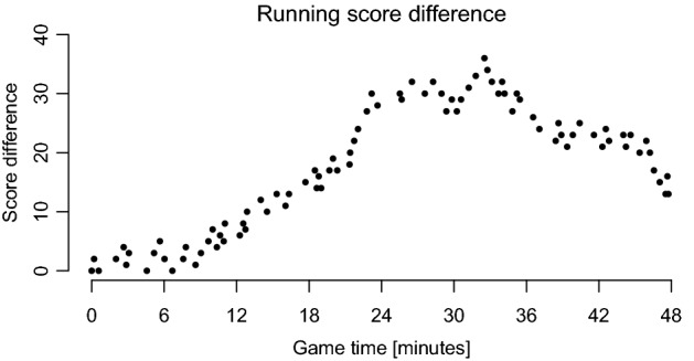
Game development in the final match of the NBA 2019–2020 season between Los Angeles Lakers and Miami Heat at October 11, 2020. Positive values indicate that LA Lakers are leading

In this manuscript, we will consider the score difference between two teams as a latent Gaussian process and use the Trend Direction Index (TDI) from Jensen and Ekstrøm (2020b) as a measure to evaluate the local probability of the monotonicity of the latent process at a given time point during a match. The Trend Direction Index uses a Bayesian framework to provide a direct answer to questions such as “What is the probability that the latent process is increasing (i.e., that one team is doing better than another) at a given time-point?”. This will allow real-time evaluation of the score difference trend at the current time-point in-game and will provide post-game inference about the “hot” periods of a match where one team outperformed the other. Furthermore, we present the Excitement Trend Index (ETI) as an objective measure of spectator excitement in a given match. The ETI is defined as the expected number of times that the score difference changes monotonicity during a match. If the score difference changes monotonicity often then that echos a game where both teams frequently score whereas a game with a low ETI will represent a one-sided match where one team is doing consistently better than the other over sustained periods of time. This manuscript expands on the ideas of the previous paper by focusing much more thoroughly on the usefulness of the ETI measure and by extending the application from analyzing a single realization to multiple realizations.

Other authors have considered using continuous processes to model the score difference of matches. Gabel and Redner (2012) shows that NBA basketball score differences are well described by a continuous-time anti-persistent random walk which suggests that a latent Gaussian process might be viable. Chen et al. (2020) consider a functional data model for dynamic behavior of cross-sectional ranks over time. While this approach can disentangle the individual and population effect on the ranks of the individual teams over time its setup is not really geared toward analyzing single matches. We use an idea similar to Chen and Fan (2018) but they do not have the same underlying Gaussian intensity process that enables us to make various Bayesian probabilistic statements throughout and after the game.

Marked point processes could be another alternative framework to model different in-game event sequences such as goals, corners or fouls in football. Narayanan et al. (2021) propose a marked point process modeling framework based on an underlying Hawkes process for inter-arrival game event times. They also employ a Bayesian framework, but their main purpose is on the predictive ability of the event times and types and how they are associated with the event intensity and not at all on the features of the underlying latent continuous process itself and how that can be used to extract aspects of the game.

The manuscript is structured as follows. In the next section we introduce trend modeling of score differences through a latent Gaussian process and define the Trend Direction Index and the Excitement Trend Index that capture the local trends in monotonicity and game excitement, respectively. Section 3 explains how to complete the model and perform estimation in practice. In Sect. 4 we apply our proposed methodology to analyze both the final match of the playoff as well as evaluating the game excitement distribution of the season by considering the ETIs from all 1143 matches from the 2019–2020 NBA season. We show how this distribution can be used to assess relative match excitement and how the ETI can be used to classify teams according to their average level of match excitement. We conclude with a discussion in Sect. 5. Materials to reproduce this manuscript and its analyses can be found at Jensen and Ekstrøm (2020a).

Methodology

Our model is based on the observed score differences $D_m(t)$ in a given match indexed by $m$ and time $t$. For each match we observe the random variables ${\mathcal{D}}_m={\left(t_{\mathit{mi}},,,D_{\mathit{mi}}\right)}_{0<i\le J_m}$ where $t_{m1}<t_{m2}<t_{\mathit{mi}}<\dots <t_{m{J}_m}$ are the ordered time points at which any team scores, $D_{\mathit{mi}}=D_m(t_{\mathit{mi}})$ is the associated difference in scores at time $t_{\mathit{mi}}$, and $J_m$ is the total number of scorings during the match. We use the convention that $D_m$ is the difference in scores of the away team with respect to the home team so that $D_m(t)>0$ means that the away team is leading at time $t$.

We assume that the observed data from a given match are noisy realizations of a latent smooth, random function defined in continuous time and evaluated at the random time points where scorings occur. Let $d_m$ be the latent function from which the realizations ${\mathcal{D}}_m$ are generated. Our objective is to infer $d_m$ and its time dynamics from ${\mathcal{D}}_m$. In pursuance of this ambition we propose the following model where $d_m$ is a Gaussian process defined on a compact subset of the real line ${\mathcal{I}}_m$ corresponding to the duration of the $m$’th game, and the observed data conditional on the scoring times and the values of the latent process at these times are independently Normally distributed random variables with a match specific variance. This model can be stated hierarchically as

$$\begin{array}{c}\hfill \begin{array}{cc}\hfill {\mathbf{\Theta }}_m\mid {\mathit{\Psi }}_m,{\mathbf{t}}_m& \sim H({\mathbf{\Theta }}_m\mid {\mathit{\Psi }}_m)\hfill \\ \hfill d_m(t)\mid {\mathbf{\Theta }}_m& \sim \mathcal{GP}({\mu }_{{\mathit{\beta }}_m}(t),C_{{\mathit{\theta }}_m}(s,t))\hfill \\ \hfill D_m(t_{\mathit{mi}})\mid d_m(t_{\mathit{mi}}),t_{\mathit{mi}},{\mathbf{\Theta }}_m& \stackrel{\mathit{iid}}{\sim }N\left(d_m,(t_{\mathit{mi}}),,,{\sigma }_m^2\right)\hfill \end{array}\end{array}$$ 1

where ${\mathbf{\Theta }}_m=({\mathit{\beta }}_m,{\mathit{\theta }}_m,{\sigma }_m^2)$ is a vector of hyper-parameters governing the dynamics of the latent Gaussian process with a prior distribution $H$ indexed by parameters ${\mathit{\Psi }}_m$, and ${\mathbf{t}}_m=(t_{m1},\dots ,t_{m{J}_m})$ is the vector of time points where scorings occur in the match. The functions ${\mu }_{{\mathit{\beta }}_m}$ on ${\mathcal{I}}_m$ and $C_{{\mathit{\theta }}_m}$ on ${\mathcal{I}}_m\times {\mathcal{I}}_m$ are the prior mean and covariance functions of the latent Gaussian process, and ${\sigma }_m^2$ is the variance characterizing the magnitude of the deviations between for the observed score differences and the values of the latent process.

A Gaussian process is characterized by the multivariate joint Normality of all of the joint distributions resulting from evaluating the process at any finite set of time points (Rasmussen and Williams 2006). Specifically, for any finite set ${\mathbf{t}}^{\ast }\subset {\mathcal{I}}_m$ it follows that the vector $d_m({\mathbf{t}}^{\ast })\mid {\mathbf{\Theta }}_m$ is distributed as $N({\mu }_{{\mathit{\beta }}_m}({\mathbf{t}}^{\ast }),C_{{\mathit{\theta }}_m}({\mathbf{t}}^{\ast },{\mathbf{t}}^{\ast }))$ where ${\mu }_{{\mathit{\beta }}_m}({\mathbf{t}}^{\ast })$ is the vector generated by evaluating the prior mean function ${\mu }_{{\mathit{\beta }}_m}(t)$ at ${\mathbf{t}}^{\ast }$ and $C_{{\mathit{\theta }}_m}({\mathbf{t}}^{\ast },{\mathbf{t}}^{\ast }))$ is the covariance matrix generated by evaluating the prior covariance function $C_{{\mathit{\theta }}_m}(s,t)$ at ${\mathbf{t}}^{\ast }\times {\mathbf{t}}^{\ast }$. Using the properties of multivariate Normal distributions, the posterior distribution $d_m({\mathbf{t}}^{\ast })\mid {\mathcal{D}}_m,{\mathbf{\Theta }}_m$ is also multivariate Normal. This facilitates Bayesian estimation of the distribution of the latent process governing the score difference given the observed data from each match.

In addition to obtaining inference for the latent process we may also estimate its time dynamics. This follows since a Gaussian process along with its time derivatives (provided they exist) are distributed as a multivariate Gaussian process (Cramer and Leadbetter 1967). We may therefore augment the hierarchical model in Eq. (1) with an additional latent structure of the first and second derivatives of $d_m$ with respect to time as

$$\begin{array}{cc}\hfill \left[\begin{array}{c}{d}_m(s)\\ d_m^{\prime }(t)\\ d_m^{″}(u)\end{array}\right]\mid {\mathbf{\Theta }}_m& \sim \mathcal{GP}\left(\left[\begin{array}{c}{\mu }_{{\mathit{\beta }}_m}(s)\\ {\mu }_{{\mathit{\beta }}_m}^{\prime }(t)\\ {\mu }_{{\mathit{\beta }}_m}^{″}(u)\end{array}\right],,,\left[\begin{array}{ccc}{C}_{{\mathit{\theta }}_m}(s,\tilde{s})& {\partial }_2{C}_{{\mathit{\theta }}_m}(s,t)& {\partial }_2^2{C}_{{\mathit{\theta }}_m}(s,u)\\ {\partial }_1{C}_{{\mathit{\theta }}_m}(t,s)& {\partial }_1{\partial }_2{C}_{{\mathit{\theta }}_m}(t,\tilde{t})& {\partial }_1{\partial }_2^2{C}_{{\mathit{\theta }}_m}(t,u)\\ {\partial }_1^2{C}_{{\mathit{\theta }}_m}(u,s)& {\partial }_1^2{\partial }_2{C}_{{\mathit{\theta }}_m}(u,t)& {\partial }_1^2{\partial }_2^2{C}_{{\mathit{\theta }}_m}(u,\tilde{u})\end{array}\right]\right)\hfill \end{array}$$ 2

where ${}^{\prime }$ and ${}^{″}$ denote the first and second time derivatives and ${\partial }_j^k$ is the $k$’th order partial derivative with respect to the $j$’th variable. Combining the models in Eqs. (1) and (2) we obtain explicit expressions for the posterior distributions $d_m^{\prime }\mid {\mathcal{D}}_m,{\mathbf{\Theta }}_m$ and $d_m^{″}\mid {\mathcal{D}}_m,{\mathbf{\Theta }}_m$. Specifically, the posterior joint distributions of the latent processes is the following multivariate Gaussian process

$$\begin{array}{c}\hfill \left[\begin{array}{c}{d}_m(s)\\ d_m^{\prime }(t)\\ d_m^{″}(u)\end{array}\right]\mid {\mathcal{D}}_m,{\mathbf{\Theta }}_m\sim \mathcal{GP}\left(\left[\begin{array}{c}{\mu }_{d_m}(s)\\ {\mu }_{d_m^{\prime }}(t)\\ {\mu }_{d_m^{″}}(u)\end{array}\right],,,\left[\begin{array}{ccc}{\mathrm{\Sigma }}_{d_m}(s,\tilde{s})& {\mathrm{\Sigma }}_{d_m{d}_m^{\prime }}(s,t)& {\mathrm{\Sigma }}_{d_m{d}_m^{″}}(s,u)\\ {\mathrm{\Sigma }}_{d_m^{\prime }{d}_m}(t,s)& {\mathrm{\Sigma }}_{d_m^{\prime }}(t,\tilde{t})& {\mathrm{\Sigma }}_{d_m^{\prime }{d}_m^{″}}(t,u)\\ {\mathrm{\Sigma }}_{d_m^{″}{d}_m}(u,s)& {\mathrm{\Sigma }}_{d_m^{″}{d}_m^{\prime }}(u,t)& {\mathrm{\Sigma }}_{d_m^{″}}(u,\tilde{u})\end{array}\right]\right)\end{array}$$ 3

where explicit expressions for the posterior mean and covariance functions are given in the online Supplementary Material. Consequently, we can sample from this posterior joint distribution at any finite number of time points as it corresponds to sampling from a certain high-dimensional Normal distribution. We utilize the posterior samples of the first and second time derivatives of the latent process to characterize the dynamical properties of each match through the Trend Direction Index and the Excitement Trend Index.

We define the Trend Direction Index (TDI) of a particular match $m$ as the local posterior probability that $d_m$ is an increasing function at any time point $t\in {\mathcal{I}}_m$. Under our model this is equal to

$$\begin{array}{c}\hfill \begin{array}{cc}\hfill {\text{TDI}}_m(t\mid {\mathbf{\Theta }}_m)& =P\left(d_m^{\prime },(t),>,0,\mid ,{\mathcal{D}}_m,,,{\mathbf{\Theta }}_m\right)\hfill \\ \hfill & =\frac{1}{2}+\frac{1}{2}\mathrm{Erf}\left(\frac{{\mu }_{d_m^{\prime }}(t)}{2^{1/2}{\mathrm{\Sigma }}_{d_m^{\prime }}{(t,t)}^{1/2}}\right)\hfill \end{array}\end{array}$$ 4

where $\mathrm{Erf}:x\mapsto 2{\pi }^{-1/2}{\int }_0^{x}exp(-u^2)\mathrm{d}u$ is the error function and ${\mu }_{d_m^{\prime }}$, and ${\mathrm{\Sigma }}_{d_m^{\prime }}$ are the posterior mean and covariance functions of the time derivative defined in Eq. (3). The interpretation of the TDI is that it quantifies the probability that one team is currently increasing the differences in scores or equivalently that they are changing the trend in their favor. A TDI equal to $50\%$ means that the game is in a stagnant state. We note that the TDI is symmetric with respect to the reference team in the definition of the score difference. If the reference team is switched, then the $\text{TDI}$ changes to $1-\text{TDI}$.

For each match we assign its Excitement Trend Index, ${\text{ETI}}_m$, as a global measure of game excitement. The index is defined as the expected number of changes in monotonicity of the posterior distribution of $d_m$ which is equivalent to the expected number of zero-crossings of the posterior distribution of $d_m^{\prime }$. We hence define

$$\begin{array}{c}\hfill \begin{array}{cc}\hfill {\text{ETI}}_m\mid {\mathbf{\Theta }}_m& =\mathrm{E}\left[\#,\left\{t,\in ,{\mathcal{I}}_m,:,d_m^{\prime },(t),=,0\right\},\mid ,{\mathcal{D}}_m,,,{\mathbf{\Theta }}_m\right]\hfill \\ \hfill & ={\int }_{{\mathcal{I}}_m}{\int }_{-\infty }^{\infty }\left|v\right|f_{d_m^{\prime }(t),d_m^{″}(t)}(0,v\mid {\mathcal{D}}_m,{\mathbf{\Theta }}_m)\text{d}v\text{d}t\hfill \\ \hfill & ={\int }_{{\mathcal{I}}_m}d{\mathrm{ETI}}_m(t\mid {\mathbf{\Theta }}_m)\mathrm{d}t\hfill \end{array}\end{array}$$ 5

where $f_{d_m^{\prime }(t),d_m^{″}(t)}(·,·\mid {\mathcal{D}}_m,{\mathbf{\Theta }}_m)$ denotes the posterior density function of $(d^{\prime },d^{″})$ at time $t$ according to Eq. (3), and $d{\mathrm{ETI}}_m$ is the instantaneous posterior probability of a zero-crossing of $d^{\prime }$ at any time point $t\in {\mathcal{I}}_m$. Integrating the instantaneous posterior probability over the duration of a match gives us the ETI. Using Eq. (3) it can be shown that the instantaneous posterior probability of a zero-crossing of $d^{\prime }$ is equal to

$$\begin{array}{c}\hfill d{\mathrm{ETI}}_m(t\mid {\mathbf{\Theta }}_m)={\lambda }_m(t)\varphi \left(\frac{{\mu }_{d_m^{\prime }}(t)}{{\mathrm{\Sigma }}_{d_m^{\prime }}{(t,t)}^{1/2}}\right)\left(2,\varphi ,\left({\zeta }_m,(t)\right),+,{\zeta }_m,(t),\mathrm{Erf},\left(\frac{{\zeta }_m(t)}{2^{1/2}}\right)\right)\end{array}$$

where $\varphi :x\mapsto 2^{-1/2}{\pi }^{-1/2}exp(-\frac{1}{2}{x}^2)$ is the standard Normal density function, and ${\lambda }_m$, ${\omega }_m$ and ${\zeta }_m$ are defined as

$$\begin{array}{cc}\hfill {\lambda }_m(t)& =\frac{{\mathrm{\Sigma }}_{d_m^{″}}{(t,t)}^{1/2}}{{\mathrm{\Sigma }}_{d_m^{\prime }}{(t,t)}^{1/2}}{\left(1,-,{\omega }_m,{(t)}^2\right)}^{1/2},{\omega }_m(t)=\frac{{\mathrm{\Sigma }}_{d_m^{\prime }{d}_m^{″}}(t,t)}{{\mathrm{\Sigma }}_{d_m^{\prime }}{(t,t)}^{1/2}{\mathrm{\Sigma }}_{d_m^{″}}{(t,t)}^{1/2}}\hfill \\ \hfill {\zeta }_m(t)& =\frac{{\mu }_{d_m^{\prime }}(t){\mathrm{\Sigma }}_{d_m^{{\prime }^{\prime }}}{(t,t)}^{1/2}{\omega }_m(t){\mathrm{\Sigma }}_{d_m^{\prime }}{(t,t)}^{-1/2}-{\mu }_{d_m^{″}}(t)}{{\mathrm{\Sigma }}_{d_m^{″}}{(t,t)}^{1/2}{\left(1,-,{\omega }_m,{(t)}^2\right)}^{1/2}}\hfill \end{array}$$

The derivation of the expression of $d{\mathrm{ETI}}_m$ can be found in the online Supplementary Material to Jensen and Ekstrøm (2020b). While no closed-form expression for ${\text{ETI}}_m\mid {\mathbf{\Theta }}_m$ seems to exist, the integration can be performed numerically. We note that the ETI is also invariant with respect to the choice of reference team in the definition of the score differences as it is defined as the expected number of both up- and down-crossings at zero of the posterior trend.

Both TDI and ETI as defined in Eqs. (4) and (5) are random variables due to their dependence on the hyper-parameters ${\mathbf{\Theta }}_m$. In our Bayesian framework these are specified under an additional layer of prior distributions according to $H({\mathbf{\Theta }}_m\mid {\mathit{\Psi }}_m)$. By fitting the model using Markov-Chain Monte Carlo methods (MCMC) we obtain samples from the posterior distribution ${\tilde{\mathbf{\Theta }}}_m\sim P({\mathbf{\Theta }}_m\mid {\mathcal{D}}_m,{\mathit{\Psi }}_m,{\mathbf{t}}_m)$ and the posterior estimates of TDI and ETI are therefore the random variables ${\text{TDI}}_m(t\mid {\tilde{\mathbf{\Theta }}}_m)$ and ${\text{ETI}}_m\mid {\tilde{\mathbf{\Theta }}}_m$.

Estimation

A completion of the model in Eq. (1) requires a specification of the prior mean and covariance functions for the latent process. The choice of these are application specific and can be based on prior knowledge of the game dynamics. We refer to the discussion in Jensen and Ekstrøm (2020b) for more information on such choices and to Sect. 3 in the same paper for a more thorough exposition on the estimation procedure.

In our application we used a constant prior mean and the squared exponential covariance function given by

$$\begin{array}{c}\hfill {\mu }_{{\mathit{\beta }}_m}(t)={\beta }_m,C_{{\mathit{\theta }}_m}(s,t)={\alpha }_m^{2}exp\left(-,\frac{{(s-t)}^2}{2{\rho }_m^2}\right)\end{array}$$

and thus ${\mathbf{\Theta }}_m=({\beta }_m,{\alpha }_m,{\rho }_m,{\sigma }_m)\in \mathbb{R}\times {\mathbb{R}}_{>0}^3$. These assumptions ensure well-defined and infinitely differentiable sample paths of $d_m$. For the hyper-parameters ${\mathbf{\Theta }}_m$ we used independent, heavy-tailed distribution with a moderate variance centered at the marginal maximum likelihood estimates of the form

$$\begin{array}{c}\hfill H({\mathbf{\Theta }}_m\mid {\mathit{\Psi }}_m)=H({\beta }_m\mid {\Psi }_{{\beta }_m})H({\alpha }_m\mid {\Psi }_{{\alpha }_m})H({\rho }_m\mid {\Psi }_{{\rho }_m})H({\sigma }_m\mid {\Psi }_{{\sigma }_m})\end{array}$$

where individual parameter distributions, H, are given by the following fairly weak priors that pose few restrictions on the initial distributions

$$\begin{array}{c}\hfill {\beta }_m\sim T_4\left(\widehat{{\beta }_m^{\text{ML}}},,,5\right),{\alpha }_m\sim T_4^{+}\left(\widehat{{\alpha }_m^{\text{ML}}},,,5\right),{\rho }_m\sim T_4^{+}\left(\widehat{{\rho }_m^{\text{ML}}},,,5\right),{\sigma }_m\sim T_4^{+}\left(\widehat{{\sigma }_m^{\text{ML}}},,,5\right)\end{array}$$

where $T_{\text{df}}$ denotes a location-scale T distribution with $\mathrm{df}$ degrees of freedom, $T_{\text{df}}^{+}$ denotes the same distribution but truncated to the positive real line, and $\widehat{{}_m^{\text{ML}}}$ notes the marginal maximum likelihood estimate of the corresponding hyper-parameter. By the properties of the model in Eq. (1) the marginal maximum log-likelihood function has the following closed-form expression

$$\begin{array}{cc}\hfill logL({\mathbf{\Theta }}_m\mid {\mathcal{D}}_m)& \propto -\frac{1}{2}log|C_{{\mathit{\theta }}_m}({\mathbf{t}}_m,{\mathbf{t}}_m)+{\sigma }_m^{2}I|\hfill \\ \hfill & -\frac{1}{2}{({\mathbf{D}}_m-{\mu }_{{\mathit{\beta }}_m}({\mathbf{t}}_m))}^T{\left[C_{{\mathit{\theta }}_m},({\mathbf{t}}_m,{\mathbf{t}}_m),+,{\sigma }_m^2,I\right]}^{-1}({\mathbf{D}}_m-{\mu }_{{\mathit{\beta }}_m}({\mathbf{t}}_m))\hfill \end{array}$$

and the marginal maximum likelihood estimates $\widehat{{\mathbf{\Theta }}_m^{\text{ML}}}={\arg \sup }_{\mathbf{\Theta }}logL(\mathbf{\Theta }\mid {\mathcal{D}}_m)$ can obtained by numerical optimization or as the roots to the score equations ${\mathrm{\nabla }}_{\mathbf{\Theta }}logL(\mathbf{\Theta }\mid {\mathcal{D}}_m)=0$.

An assessment of the validity of the distributional assumptions of our model can be performed by a comparison of the quantiles of the posterior predictive distribution with the observed data similar to the method proposed by Dunn and Smyth (1996). We note that while Gaussianity is required for the latent function, the likelihood (conditional distribution of the observations given the latent function) is not required to be Normal distributed but this can be adapted to a specific situation. Once we have this estimate it can be plugged into the expressions for the posterior distributions in order for the Markov chain Monte Carlo procedure to provide predictions that can be used to compute the posterior distributions (Jensen and Ekstrøm 2020b).

We have implemented our model in the probabilistic programming language Stan (Carpenter et al. 2017) that uses a Hamiltonian Markov Chain Monte Carlo algorithm to sample from the distributions of ${\text{TDI}}_m(t\mid {\tilde{\mathbf{\Theta }}}_m)$ and $d{\mathrm{ETI}}_m(t\mid {\tilde{\mathbf{\Theta }}}_m)$ on any finite set of time points in ${\mathcal{I}}_m$. Posterior summary measures of ${\text{TDI}}_m(t\mid {\tilde{\mathbf{\Theta }}}_m)$ and ${\mathrm{ETI}}_m\mid {\tilde{\mathbf{\Theta }}}_m$ can then be calculated and reported from the posterior samples as, e.g., the mean or median along with $(1-\alpha )100\%$ credible intervals. Formula (8) in Jensen and Ekstrøm (2020b) provides a detailed representation of the posterior distribution of the hyper-parameters and information on how the TDI, the ETI and their credibility intervals are calculated in practice.

Application: the 2019–2020 NBA basketball season

To illustrate the applicability of our proposed methodology we apply it to data from all regular games from the 2019–2020 NBA basketball season. The data were obtained from Sports Reference (2020) and is provided in Jensen and Ekstrøm (2020a). A lot of points are scored during a basketball match so it is easy to see the development of the score difference in a single match.

The 2019–2020 NBA season was suspended mid-March due to COVID-19 but it was resumed again in July 2020. There were a total of 1059 regular season matches. The subsequent playoffs comprised 84 matches including the final for a grand total of 1143 matches. For ease of comparison we are only considering the first 48 regular minutes of each match—any part of a match that goes into overtime will be disregarded, and we hence let ${\mathcal{I}}_m=[0;48]$ minutes.

We wish to use the trend analysis proposed for three purposes: 1) to show how the TDI can be used to infer real-time and post-game evaluation of the trends in a match. 2) To evaluate the ETI for all 1143 matches in the 2019–2020 season to provide background and reference information about the matches, and 3) to summarize ETI at the team level in order to identify groups of teams more/less likely to give an exciting game.

For each match we used the prior specification from Sect. 3. We ran four independent chains for 50,000 iterations each with half of the iterations used for warm-up and evaluated the posterior distribution of ${\text{TDI}}_m(t\mid {\tilde{\mathbf{\Theta }}}_m)$ and $d{\mathrm{ETI}}_m(t\mid {\tilde{\mathbf{\Theta }}}_m)$ on an equidistant grid of 241 time points in $[0;48]$. The posterior distribution of ${\text{ETI}}_m\mid {\tilde{\mathbf{\Theta }}}_m$ was calculated by numerical integration using the trapezoidal method.

For our first purpose of analyzing trends in individuals matches we consider the final match of the 2019–2020 season. The raw data for the running score difference between LA Lakers and Miami Heat was shown in Fig. 1. Figure 2 shows the results from the post-game analysis.

Fig. 2.

Results from fitting the latent Gaussian Process to the final match between LA Lakers and Miami Heat in the 2019–2020 NBA season. Larger values in running score differences and the Trend Direction Index reflect the situation where LA Lakers are doing better. The top left panel shows the posterior distribution of the the latent process with the posterior means in bold. The gray areas show point-wise credible and posterior prediction intervals. The top right panel provides similar information for the the posterior trend. The bottom left panel shows the TDI (in percent) and can be used to read off probability statements about the trends in the running score difference. The bottom right panel shows the local ETI and quantifies the instantaneous probability of a change in monotonicity of the score differences

Evaluating the game trends from the TDI in Fig. 2 shows that LA Lakers had control of most of the match since the posterior probability of a positive trend was high throughout most of the match. Only toward the end of the third quarter did Miami Heat gain the upper hand and had a period where they fought back. The same overall patterns could be seen from Fig. 1, but we are now able to assign uncertainties and make objective evaluations of the overall trend and its local properties. In the fourth quarter from around 38 minutes to 43 minutes we can see that mean TDI increases to over 80% but the probability interval is very wide reflecting that it is difficult to say whether the trend is increasing or if it might as well just be random fluctuations in scores. Similarly for the first half of the third quarter. Teams wishing to evaluate the match should primarily concentrate on periods where the latent trend and its probability interval is either close to 50% or when the trend is disadvantageous for the team. The spikes observed in the local ETI (lower right plot of Fig. 2) indicate the time points where the monotonicity of the underlying trend is changing sign, with higher values of $d$ETI representing more steep changes.

To evaluate the overall distribution of the ETIs we fitted our model to each of the 1143 matches during the season and estimated the ETI for each. The results are summarized in the left panel of Fig. 3 showing the marginal distribution of the median posterior ETIs. The solid line shows the fit of a Gaussian mixture model with four components, where the number of components were determined by sequential bootstrapped likelihood ratio tests (Scrucca et al. 2016). The marginal distribution of the posterior median ETIs is right skewed (skewness = 0.52) with a range of [0.19; 26.23], and a median of 10.12 (mean = 10.64, SD = 4.51). This implies that the time-varying score differences of the games in the season changes monotonicity approximately ten times during a game on average but with a large variation between matches. For comparison, the final match between LA Lakers and Miami Heat shown in Fig. 2 has a median posterior ETI of $6.71$.

Fig. 3.

Histogram and Gaussian mixture model estimate of the distribution of the 1143 median posterior ETIs from the NBA 2019–2020 season (left panel) and the median posterior ETIs as a function of calendar time from October 22, 2019 to October 11, 2020 (right panel)

We wished to examine if there was a calendar time effect on game excitement as the season progressed in order to investigate if we would find that games became more exciting as the teams fought to stay in the competition to enter the final playoffs or if we could detect fatigue over the season. The right panel of Fig. 3 shows the median posterior ETIs as a function of calendar time at which the matches were played. Besides illustrating the gap from the COVID-19 hiatus, the figure shows that the excitement indices are relatively evenly distributed throughout the season.

When matches are ranked from lowest to highest median posterior ETI, we can extract the individual analyses for matches representing the full span of the ETI range. Figure 4 shows the analysis results of our proposed method for the matches with minimum, first, second, third quantile, and maximum median posterior ETI. It is clear from the observed running score differences, posterior trends, and the TDIs that these five matches represent substantially different game experiences.

Fig. 4.

Observed score differences with posteriors of the latent processes (left panels), posterior trends (middle panels) and posterior Trend Direction Indices (right panels) for five games from the NBA season 2019–2020 with median posterior Excitement Trend Indices corresponding to the 0%, 25%, 50%, 75%, and 100% percentiles of the distribution of all games in the season. Gray regions depict 50% and 95% point-wise credible intervals and 95% posterior prediction intervals

The first row of Fig. 4 for Dallas Mavericks vs the Golden State Warriors show a very one-sided match leading to the minimum ETI during the season. The third row of Fig. 4 for the LA Clippers vs Charlotte Hornets match indicates that while the Hornets did lead throughout most of first quarter, the Clippers reversed the game toward the end of first quarter and kept the lead through most of second quarter. After that the Hornets started to keep the lead and the Clippers never managed to make a proper comeback and the game trend was rather flat in the last two quarters of the game since the two teams more or less kept the pace with each other except for the effort shown midway in quarter four. In contrast, the match between New Orleans Pelicans vs Utah Jazz (fifth row in Fig. 4) showed trends that varied direction frequently and where the TDI showed alternating periods of scoring bursts making it a very exciting and unpredictable game. The online Supplementary Material lists summary statistics of the estimated ETIs for all 1143 matches.

Summarizing the median posterior ETIs at the team level across all matches during the season lead to comparable values for all 30 teams. Table 1 shows the summary statistics for all 30 teams ordered by their season average excitement. The New Orleans Pelicans had the highest median posterior ETI averaged over the season with an average median posterior ETI of 11.67 (SD = 4.91, IQR = $[3.10;23.54]$), while the Charlotte Hornets had the lowest average median posterior ETI with a value of 9.26 (SD = 3.74, IQR = $[1.96;15.95]$). The small fluctuation of the averages suggests that the teams are comparable in terms of excitement when averaging across all their games during the season, and that the major source of variation in excitement during the season (as seen in Fig. 3) is governed by the specific matches.

Table 1.

Team specific median posterior Excitement Trend Indices summarized across all their matches in the 2019–2020 NBA season and ordered by the season average

	Average	SD	2.5%	50%	97.5%	Group
New Orleans Pelicans	11.67	4.91	3.10	11.59	23.54	A
Washington Wizards	11.36	4.46	2.98	11.63	18.28	A
San Antonio Spurs	11.31	5.31	3.52	9.88	23.44	A
Oklahoma City Thunder	11.26	5.32	1.68	11.55	23.74	A
Portland Trail Blazers	11.21	4.46	3.31	10.82	18.48	A
Los Angeles Lakers	11.16	4.43	3.61	10.52	19.79	A
Philadelphia 76ers	11.09	4.70	2.73	10.28	21.53	A
Minnesota Timberwolves	11.09	4.28	4.01	10.69	19.46	A
Utah Jazz	10.96	5.44	3.09	9.76	23.54	A
Memphis Grizzlies	10.94	4.59	3.04	10.36	20.84	A
Cleveland Cavaliers	10.90	4.50	4.93	10.39	22.36	A
Toronto Raptors	10.69	4.44	3.48	10.33	21.79	B
Houston Rockets	10.67	4.12	3.52	10.74	19.17	B
Chicago Bulls	10.66	3.98	2.95	10.65	17.49	B
Boston Celtics	10.61	4.66	2.81	10.19	20.92	B
Orlando Magic	10.56	4.89	2.72	10.41	21.01	B
Milwaukee Bucks	10.55	4.36	2.77	9.59	18.13	B
Los Angeles Clippers	10.54	4.14	4.05	10.72	20.56	B
Miami Heat	10.44	4.29	3.28	9.91	18.54	B
Golden State Warriors	10.40	4.58	3.37	10.24	18.72	B
Indiana Pacers	10.37	3.99	3.31	10.22	18.54	B
Brooklyn Nets	10.33	4.57	3.07	10.06	18.89	C
Dallas Mavericks	10.27	4.99	3.00	9.04	22.09	C
Atlanta Hawks	10.26	4.35	2.50	9.75	18.31	C
Phoenix Suns	10.25	4.32	3.78	9.29	19.81	C
Denver Nuggets	10.16	4.39	3.42	9.59	19.61	C
New York Knicks	10.11	4.05	2.84	9.87	18.47	C
Sacramento Kings	9.94	4.19	3.66	9.30	18.93	C
Detroit Pistons	9.86	4.00	3.73	9.44	17.08	C
Charlotte Hornets	9.26	3.74	1.96	9.22	15.95	D

The group column shows the clustering induced by our optimization procedure

Although the team averages in Table 1 show limited variability it is of interest to estimate a number of subgroups among the teams that exhibited similar degree of excitement on average during the season—effectively clustering the teams. This would enable fans, promoters, and sponsors to infer which teams were more likely to partake in an exciting game. The problem is mathematically equivalent to looking at the relationship between the median posterior ETIs as the outcome in a linear regression model where the explanatory categorical variable ranges over the set of all partitions of the 30 teams, and as the objective we seek the smallest number of partitions that best explains the observed outcome by comparing all possible splits of the ranked teams for a given number of partitions. This will then define subgroups of teams.

As the optimization criterion for the subgroup identification we used the root-mean-squared error of prediction based on leave-one-out cross-validation, denoted ${\text{RMSEP}}_{\text{LOO-CV}}^{C=c}$ where $c$ is the number of subgroups. Our sequential optimization procedure showed that the optimization criterion stabilized at four subgroups: ${\text{RMSEP}}_{\text{LOO-CV}}^{C=2}=4.493$, ${\text{RMSEP}}_{\text{LOO-CV}}^{C=3}=4.49$, ${\text{RMSEP}}_{\text{LOO-CV}}^{C=4}=4.489$, and subsequently for $C=5,\dots ,8$ it remained at the same value. The labels of these groups are shown in the rightmost column in Table 1. The result is thus an identification of three change-points in the ranking of the teams according to median posterior ETI averaged across the season. The most noticeable result is that Charlotte Hornets constitute a singleton since that team has substantial lower ETI than the team with the second lowest ETI. To maximize the probability of seeing an exciting game it would thus have be wise to avoid matches in which the Hornets were playing.

Figure 5 shows the estimated linear association between the seasonal standard deviations and average of the median posterior ETIs for each team. The teams follow a straight line through the origin fairly well, suggesting that the coefficient of variation is fairly constant across the teams. This also suggests that teams with large seasonal average excitement are also more likely to be part of really spectacular matches. Teams consistently contributing with highly exciting matches during the season should therefore be represented in the bottom right part of the plot. Assessing which teams that where generally most exiting to watch during the season is thus a bias-variance trade-off decision. While the New Orleans Pelicans were most exciting on average, the Washington Wizards where second-most exciting on average but also had a notably lower seasonal standard deviation. This means that although the latter team was less exciting on average during the season, their level of excitement was more stable throughout. On the other hand, the San Antonio Spurs had the third largest average excitement but simultaneously also a much larger standard deviation making the excitement of their individual matches much less reliable throughout the season.

Fig. 5.

Seasonal SD of the estimated ETIs plotted against the average estimated ETI for each team. Shapes/colors indicate ETI groups. The line represents the best linear regression line through the origin. The plot suggests a linear relationship between the SDs and averages indicating a fairly constant coefficient of variation. Teams with higher excitement trend index are more likely to have higher variation in their excitement scores

Discussion

We have introduced the Trend Direction Index as a measure to estimate and evaluate the trends in running score difference in sports. The Trend Direction Index is based on a latent Gaussian process model and enables us to make Bayesian in-game and post-game evaluations about the underlying trends in scoring patterns and to attach easily interpretable probability statements to the results. In addition we have presented the Excitement Trend Index as the expected number of monotonicity changes in the underlying trend and we showed how it can be used to gauge how exciting a match will be: if one team is consistently outperforming the other then the match quickly becomes one-sided and less exciting. Both indices have intuitive interpretations that are easily conveyed to non-statisticians, coaches, players, and commentators.

We have showed how the proposed method can be used to analyze single matches in order to determine strategies to identify periods throughout the game where the momentum of the game changes. The model utilizing the latent trend enables a highly detailed modeling approach where game development can be followed from minute to minute. This will facilitate and improve post-game coaching and influence future game tactics. While the computations for a single game are easily accomplishable on a standard laptop, it may require a high-speed computing cluster to obtain real-time results during a match. However that should not prove prohibitive for high-end matches. With a small number of data points our model will—like any statistical model—primarily be dominated by the prior which is why the method proposed may be better suited to types of games where there are frequent updates on the scoring.

It should be stressed that we are using a Gaussian process to model score differences that in reality are integer-valued. This approximation of an integer-based outcome by a model accommodating continuous values is not uncommon in statistics and it is hardly a problem when the purpose is estimating the distribution of a continuous latent process. A small efficiency gain might be obtained if a model addressing integer outcomes such as a Skellam distribution was used directly on top of the Gaussian process. We have a similar extension outlined in Jensen and Ekstrøm (2020b) which had no impact on the estimated trend, but the computation time was substantially longer.

Our analysis of all matches in the 2019–2020 NBA season showed that different values of the ETI captured games with vastly different features and showed that it could be used as a tool to discriminate the teams. In this case, the latent Gaussian process benefits greatly from the large numbers of scorings that are typical in basketball, since that means that there will be a large and frequent number of observations within each match that the model can utilize. In contrast, sports with few scorings such as soccer may prove a more difficult task simply because there is very few changes in the running score throughout a match.

There are a couple of future research ideas that could extend our current approach of using the latent Gaussian trend to infer measures for game excitement. One idea is to define a weighted version of the Excitement Trend Index, ${\mathrm{wETI}}_m$, so that changes in monotonicity of the score differences are i) weighted higher toward the end of the game and ii) weighted lower if one team is already far away of the other team as measured by the absolute value of the posterior mean ${\mu }_{d_m}$. This motivates a modification of the definition of the ETI in Eq. (5) to the following weighted form

$$\begin{array}{c}\hfill {\mathrm{wETI}}_m\mid {\mathbf{\Theta }}_m={\int }_{{\mathcal{I}}_m}d{\mathrm{ETI}}_m(t\mid {\mathbf{\Theta }}_m)w(t,|{\mu }_{d_m}(t)|)\mathrm{d}t\end{array}$$

where $w:{\mathcal{I}}_m\times {\mathbb{R}}_{\ge 0}\mapsto {\mathbb{R}}_{\ge 0}$ is a weight function that is increasing in its first variable and decreasing in its second variable. Such weight functions could be constructed as a product of two kernel functions defined on their individual domains and with bandwidths based on studies of psychological perception.

Another approach for quantifying excitement would be to define it at the team-level instead of at the match level. In that case one could define team-specific Trend Excitement Indices nested with a match by looking at both the up- and down-crossing of $d{f}_m$ at zero. This would result in two excitement indices for each match, $({\mathrm{ETI}}_{\mathit{am}},{\mathrm{ETI}}_{\mathit{bm}})$ for teams $a$ and $b$ which would reflect how exciting each team were in match $m$ with respect to changing the sign of the score differences in their favor.

The proposed methodology readily opens up new venues for more extensive analyses. One possibility would be to let the ETI be studied as a function of time since the excitement might easily change depending on the point in time of the game and as the match nears the end. For games like basketball it might also be possible to modify the analyses to compare ETI across quarters to determine if some periods of the game are generally more likely to be exciting than others. This particion of the time interval, however, would require that the starting point of each quarter could be non-zero and would match the corresponding previous end score.

In our application we have clustered the teams into four categories based on their individual marginal ETI scores. While that provides a way to group the teams, it seems natural to consider the ETI for pairs of teams since both teams contribute to making the game more exciting. Thus, some matches between specific teams such as long-running rivals or teams that are close to each other on the score board might be more inclined to result in more interesting matches and in higher ETI scores. Adapting the cluster analysis to accommodate pairs of teams instead of individual teams would be one way to pursue this in future research.

Finally, the proposed method uses the score difference as the only input to estimate the underlying Gaussian trend process. Our model could be extended to include several types of game events simultaneously—score differences, absolute score level, scoring attempts, ball passes—in order to estimate a shared underlying latent process that could be used to evaluate the game excitement. This would also render the proposed method more responsive to games that naturally contain fewer scorings since additional information can be gained from the other input variables.

In conclusion, we have provided an analytical framework for analyzing the trend in the running score difference in sports matches. The latent Gaussian process model requires very few assumptions which makes the modeling approach very flexible and applicable to a multitude of sports.

Supplementary Information

Below is the link to the electronic supplementary material.

Funding

The research was funded by the University of Copenhagen.

Data availibility

All data are available at https://github.com/aejensen/Having-a-Ball.

Code availability

All code are available at https://github.com/aejensen/Having-a-Ball and https://github.com/aejensen/TrendinessOfTrends.

Declarations

Conflict of interest

The authors declare that they have no conflict of interest.

References

- Baboota R, Kaur H. Predictive analysis and modelling football results using machine learning approach for english premier league. Int. J. Forecast. 2018 doi: 10.1016/j.ijforecast.2018.01.003. [DOI] [Google Scholar]
- Carpenter, Bob, Gelman, Andrew, Hoffman, Matthew D., Lee, Daniel, Goodrich, Ben, Betancourt, Michael, Brubaker, Marcus, Guo, Jiqiang, Li, Peter, Riddell, Allen: Stan: a probabilistic programming language. J. Stat. Softw. 76(1) (2017) [DOI] [PMC free article] [PubMed]
- Cattelan M, Varin C, Firth D. Dynamic bradley-terry modelling of sports tournaments. J. R. Stat. Soc. Ser. C (Appl. Stat.) 2013;62(1):135–50. doi: 10.1111/j.1467-9876.2012.01046.x. [DOI] [Google Scholar]
- Chen T, Fan Q. A functional data approach to model score difference process in professional basketball games. J. Appl. Stat. 2018;45(1):112–27. doi: 10.1080/02664763.2016.1268106. [DOI] [Google Scholar]
- Chen Y, Dawson M, Müller H-G. Rank dynamics for functional data. Comput. Stat. Data Anal. 2020;149:106963. doi: 10.1016/j.csda.2020.106963. [DOI] [Google Scholar]
- Cramer, H., Leadbetter, M.R.: Stationary and Related Stochastic Processes: Sample Function Properties and Their Applications. Wiley, Berlin (1967)
- Dunn PK, Smyth GK. Randomized quantile residuals. J. Comput. Graph. Stat. 1996;5(3):236–44. [Google Scholar]
- Ekstrøm CT, Van Eetvelde H, Ley C, Brefeld U. Evaluating one-shot tournament predictions. J. Sports Anal. 2020 doi: 10.3233/JSA-200454. [DOI] [Google Scholar]
- Gabel, A., Redner, S.: Random walk picture of basketball scoring. J. Quant. Anal. Sports 8(1)
- Groll A, Ley C, Schauberger G, Van Eetvelde H. A hybrid random forest to predict soccer matches in international tournaments. J. Quant. Anal. Sports. 2019;15:271–88. doi: 10.1515/jqas-2018-0060. [DOI] [Google Scholar]
- Gu W, Saaty TL. Predicting the outcome of a tennis tournament: based on both data and judgments. J. Syst. Sci. Syst. Eng. 2019;28(3):317–43. doi: 10.1007/s11518-018-5395-3. [DOI] [Google Scholar]
- Jensen, A.K., Ekstrøm, C.T.: GitHub repository for having a ball. https://github.com/aejensen/Having-a-Ball (2020a)
- Jensen, A.K., Ekstrøm, C.T.: Quantifying the trendiness of trends. J. R. Stat. Soc. Ser. C (2020b) [DOI] [PMC free article] [PubMed]
- Karlis D, Ntzoufras I. Analysis of sports data by using bivariate poisson models. J. R. Stat. Soc. Ser. D (Stat.) 2003;52(3):381–93. doi: 10.1111/1467-9884.00366. [DOI] [Google Scholar]
- Narayanan, S., Kosmidis, I., Dellaportas, P.: Flexible marked spatio-temporal point processes with applications to event sequences from association football. arXiv:2103.04647v1, pp. 1–36. arXiv:2103.04647 (2021)
- Rasmussen, C.E., Williams, C.K.I.: Gaussian Processes in Machine Learning. MIT Press (2006)
- Scrucca L, Michael Fop T, Murphy B, Raftery AE. mclust 5: clustering, classification and density estimation using gaussian finite mixture models. R J. 2016;8(1):289–317. doi: 10.32614/RJ-2016-021. [DOI] [PMC free article] [PubMed] [Google Scholar]
- Sports Reference LLC. Basketball reference. https://www.basketball-reference.com/ (2020)
Associated Data
This section collects any data citations, data availability statements, or supplementary materials included in this article.
Supplementary Materials
Data Availability Statement