The effects of frequency-dependent attenuation and dispersion on sound speed measurements: applications in human trabecular bone

Abstract

Sound speed may be measured by comparing the transit time of a broadband ultrasonic pulse transmitted through an object with that transmitted through a reference water path. If the speed of sound in water and the thickness of the sample are known, the speed of sound in the object may be computed. In order to measure the transit time differential, a marker such as a zero crossing may be used. A sound speed difference between the object and water shifts all markers backward or forward. Frequency-dependent attenuation and dispersion may alter the spectral characteristics of the waveform, thereby distorting the locations of markers and introducing variations in sound-speed estimates. Theory is derived to correct for this distortion for Gaussian pulses propagating through linearly-attenuating, weakly-dispersive media. The theory is validated using numerical analysis, measurements on a tissue mimicking phantom, and on 24 human calcaneus samples in vitro. Variations in soft-tissue-like media are generally not exceptionally large for most applications but can be substantial, particularly for high bandwidth pulses propagating through media with high attenuation coefficients. At 500 kHz, variations in velocity estimates in bone can be very substantial - on the order of 40–50 m/s - due to the high attenuation coefficient of bone. In trabecular bone, the effects of frequency-dependent attenuation are considerable while the effects of dispersion are negligible.

Introduction

Sound speed is a fundamental property that has been measured in many soft tissues and conveys important information regarding tissue composition.^1–5 Variations in sound speed exhibit a dependence on water^6,7 content in human brain and water⁸ and fat^8,9 contents in human liver. At very high frequencies (100 MHz), sound speed in rat liver shows systematic variations with fat,^10,11 protein,¹¹ and water¹¹ contents. Collagen content is another important determinant of velocity in collagen-rich tissues.^12–14

In addition to its importance in soft tissues, sound speed has been demonstrated to be highly correlated with calcaneal mass density^15–22 which is in turn related to systemic osteoporotic fracture risk.²³ Many commercial bone sonometers capitalize on this phenomenon. Calcaneal ultrasonic measurements (sound speed combined with broadband ultrasonic attenuation) have been shown to perform well for prediction of hip fractures in women in prospective^24,25 and retrospective^26–29 studies. While the calcaneus is composed mainly of trabecular bone, sound speed has also been used to characterize material properties of cortical bone.^30–33

Many ultrasonic velocity measurements, including those incorporated into most commercial bone sonometers, are based on time-of-flight measurements. The transit time of ultrasound through tissue is compared with the transit time through water. With knowledge of the speed of sound in water and the thickness of the sample (e.g. calcaneus), the speed of sound in the sample may be computed. In order to measure transit time, a particular marker (e.g. a zero-crossing, maximum, or minimum) between the leading and trailing edges on the reference and data waveforms is designated. The difference in arrival times for this marker is then used to compute sound speed. For media that exhibit frequency-dependent attenuation, however, the pulse spreads over time and the magnitude of estimate of the difference in arrival times depends on the point in the waveform analyzed. This is particularly problematic for highly attenuating media such as bone.

In general, the velocity of sound in a medium may depend on ultrasonic frequency. In this case, it is important to consider differences among phase velocity (the velocity of a single-frequency component), group velocity (the velocity of the center of a pulse), and signal velocity (the velocity of the front of a pulse).³⁴ The frequency dependence of phase velocity (dispersion) can alter the pulse shape during propagation, thereby altering zero crossing locations and affecting sound speed estimates.

There is substantial variation in choice for designated markers in the literature including the leading edge (first detectable deviation from zero) of received ultrasonic pulse,^18,35–37 thresholding at 10% of the maximum value,³⁷ thresholding at 3 times the noise standard deviation,³⁸ first zero crossing,^20,22,37 “specific” zero crossings,¹⁵ first through fourth zero crossing, first and second maxima and minima,³⁹ and zero crossing of the first negative slope.⁴⁰ These techniques provide sound speed estimates which usually lie somewhere between signal velocity and group velocity.

Some investigators^37,39,41 have reported inconsistencies with sound speed estimates in bone with zero-crossing techniques and have qualitatively attributed them to spectral changes arising from frequency dependent attenuation and dispersion. This ambiguity constitutes one argument in favor of phase velocity, which is measured in frequency domain, as opposed to group or signal velocity measurements, which are measured in time domain.^37,41,42 Since the majority of clinical validation studies of speed of sound as a diagnostic tool are based on time-domain measurements, however, group and signal velocity measurement techniques continue to be of high interest. Errors in sound speed estimates due to frequency dependent attenuation in nondispersive media have previously been investigated theoretically.⁴³

This paper is organized as follows. First, theory is derived to compensate for variations in transit-time-based sound speed estimates for Gaussian pulses propagating through linearly-attenuating, weakly-dispersive media. It is shown that measurements become independent of marker choice if properly compensated. Then, validation experiments using measurements on a tissue mimicking phantom and on 24 human calcaneus samples in vitro are described. Finally, the theory and results are discussed.

Theory

To measure sound speed, arrival times of received through-transmission broadband pulses may be measured with and without the sample in the water path. Sound speed in a sample, c_s, may then be computed from

$$c_s=\frac{c_w}{1+\frac{c_w\Delta t}{d}}$$ (1)

where d is the thickness of the sample, Δt is the difference in arrival times, and c_w is the speed of sound in water.

The effect of frequency-dependent attenuation and pulse marker designation on transit time estimation is illustrated in Figure 1. A hypothetical reference (through water) waveform is shown in the top part of the figure. Below is the waveform corresponding to the measurement through a sample with faster speed of sound than water (hence the earlier arrival time) and linear frequency-dependent attenuation (hence the lower frequency and longer period). The difference in transit time between the two waveforms depends on which marker is adopted. The closer a marker is to the leading edge of the pulse, the greater the measured time differential and the faster the speed of sound estimate.

1.

The effect of frequency-dependent attenuation and pulse marker designation on transit time estimation. The reference (through water) waveform is shown above. Below is the waveform corresponding to the measurement through a sample with faster speed of sound than water (hence the earlier arrival time) and linear frequency-dependent attenuation (hence the lower frequency and longer period). The difference in transit time between the two waveforms depends on which marker is utilized.

The effects of attenuation and phase-shifting due to differences in sound speeds between water and sample are modeled here as a linear filtering process where x(t) is the reference signal through water, h(t) is the impulse response of the linear filtering process, and y(t) is the radio frequency signal recorded with the sample in the water path.

$$y(t)=h(t)*x(t)$$ (2)

The transfer function of the medium is

$$H(f)=e^{-\beta fd}{e}^{-i2\pi f\Delta t(f)}$$ (3)

where f is frequency, β is the attenuation coefficient of the medium, d is the thickness of the sample, and Δt(f) is the time delay (relative to a water reference signal) at a given frequency due to a difference in sound speed between the sample and reference given by

$$\Delta t(f)=d\left[\frac{1}{c_s(f)}-\frac{1}{c_w}\right]$$ (4)

where c_w is the speed of sound in water (assumed to be nondispersive) and c_s(f) is the frequency-dependent sound speed in the dispersive medium.

The input or reference signal, x(t), is assumed to be a Gaussian modulated sinusoid. The analytic signal representation is given by

$$x(t)=A{e}^{-t^2/2{\sigma }_t^2}{e}^{i2\pi f_{0}t}{e}^{i{\varphi }_0}$$ (5)

where A is the amplitude, σ_t is a measure of the duration of the pulse, and f₀ is the center frequency. Take the Fourier transform.

$$X(f)=A{\sigma }_t\sqrt{2\pi }{e}^{-{(f-f_0)}^2/2{\sigma }_f^2}{e}^{i{\varphi }_0}$$ (6)

where σ_f = 1/(2πσ_t) is a measure of the bandwidth. Now the Fourier Transform of the signal recorded with the sample in the water path is given by

$$Y(f)=H(f)X(f)=A{\sigma }_t\sqrt{2\pi }{e}^{-{(f-f_0)}^2/2{\sigma }_f^2}{e}^{-\beta fd}{e}^{-i2\pi f\Delta t(f)}{e}^{i{\varphi }_0}$$ (7)

The product of the first two exponentials may be expressed as a single exponential. The resulting exponent may be simplified by completing the square⁴⁴ and is then given by

$$-\frac{{(f-f_0)}^2}{2{\sigma }_f^2}-\beta fd=-\frac{f^2-2(f_0-{\sigma }_f^2\beta d)f+f_0^2}{2{\sigma }_f^2}=-\frac{{(f-f_1)}^2-f_1^2+f_0^2}{2{\sigma }_f^2}$$ (8)

where f₁ is the new (down-shifted) center frequency given by

$$f_1=f_0-{\sigma }_f^2\beta d.$$ (9)

Note that the bandwidth of the pulse is unchanged by a medium in which attenuation is proportional to frequency.⁴⁴ The Fourier transform of the signal recorded with the sample in the water path is now given by

$$Y(f)=A{\sigma }_t\sqrt{2\pi }{e}^{(f_1^2-f_0^2)/2{\sigma }_f^2}{e}^{-{(f-f_1)}^2/2{\sigma }_f^2}{e}^{-i2\pi f\Delta t(f)}{e}^{i{\varphi }_0}$$ (10)

From the Kramers-Kronig relationship between ultrasonic attenuation and phase velocity, a medium (such as bone) which exhibits an attenuation coefficient which has a linear dependence on frequency would be expected to exhibit a phase velocity with a logarithmic dependence on frequency.⁴⁵ However, over a relatively narrow range of frequencies of interrogation, this dispersion may be assumed to be approximately linear. This is consistent with published investigations.^37,42

$$c_s(f)=c_s(f_0)+b_s(f-f_0)$$ (11)

If the dispersion is relatively weak, i.e. b_s(f-f₀)/c_s(f₀) << 1, then the reciprocal in Equation (4) may be written as

$$\frac{1}{c_s(f)}=\frac{1}{c_s(f_0)}\frac{1}{\left[1+\frac{b_s}{c_s(f_0)}(f-f_0)\right]}\approx \frac{1}{c_s(f_0)}\left[1-\frac{b_s}{c_s(f_0)}(f-f_0)\right]$$ (12)

Now, time delay, Δt, becomes

$$\Delta t(f)=d\left[\frac{1}{c_s(f_0)}-\frac{b_s}{c_s^2(f_0)}(f-f_0)-\frac{1}{c_w}\right]=\Delta t(f_0)-g(f-f_0)$$ (13)

where g = db_s/c_s²(f₀). Now the Fourier transform of the signal may be written

$$Y(f)=A{\sigma }_t\sqrt{2\pi }{e}^{(f_1^2-f_0^2)/2{\sigma }_f^2}{e}^{-{(f-f_1)}^2/2{\sigma }_f^2}{e}^{-i2\pi f\Delta t(f_0)}{e}^{i2\pi fg(f-f_0)}{e}^{i{\varphi }_0}$$ (14)

For weak dispersion, the second to the last exponential may be approximated by the first two terms of a Taylor expansion,

$$e^{i2\pi fg(f-f_0)}\approx 1+i2\pi fg(f-f_0)=1-i2\pi g{f}_{0}f+i2\pi g{f}^2$$ (15)

Now Equation (14) may be rewritten

$$Y(f)=A{e}^{(f_1^2-f_0^2)/2{\sigma }_f^2}{e}^{i{\varphi }_0}(1-i2\pi g{f}_{0}f+i2\pi g{f}^2)Z(f)$$ (16)

where

$$Z(f)={\sigma }_t\sqrt{2\pi }{e}^{-{(f-f_1)}^2/2{\sigma }_f^2}{e}^{-i2\pi f\Delta t(f_0)}$$ (17)

The Derivative theorem of Fourier analysis states that if w(t) and W(f) constitute a Fourier transform pair, then the n^th derivative, w⁽ⁿ⁾(t), and (i2πf)ⁿW(f) also constitute a Fourier transform pair.⁴⁶ Taking the inverse Fourier transform of Equation 16,

$$y(t)=A{e}^{(f_1^2-f_0^2)/2{\sigma }_f^2}{e}^{i{\varphi }_0}[z(t)-g{f}_0{z}^{\prime }(t)-i(g/2\pi ){z^{\prime }}^{\prime }(t)]$$ (18)

The inverse Fourier transform of Z(f) is given by

$$z(t)={\sigma }_t\sqrt{2\pi }\sqrt{2\pi }{\sigma }_f{e}^{i2\pi f_1[t-\Delta t(f_0)]}{e}^{-2{\pi }^2{\sigma }_f^2{[t-\Delta t(f_0)]}^2}=e^{i2\pi f_1[t-\Delta t(f_0)]}{e}^{-{[t-\Delta t(f_0)]}^2/2{\sigma }_t^2}$$ (19)

The derivatives of z(t) are given by

$$z^{\prime }(t)=z(t)\left[i2\pi f_1-\frac{t-\Delta t(f_0)}{{\sigma }_t^2}\right]$$ (20)

$$z^{″}(t)=z^{\prime }(t)\left[i2\pi f_1-\frac{t-\Delta t(f_0)}{{\sigma }_t^2}\right]+z(t)\left(\frac{-1}{{\sigma }_t^2}\right)=z(t)\left\{{\left[i2\pi f_1-\frac{t-\Delta t(f_0)}{{\sigma }_t^2}\right]}^2-\frac{1}{{\sigma }_t^2}\right\}$$ (21)

In determining the locations of zero crossings, the phase of y(t) is the main concern.

$$Arg\left[y(t)\right]={\varphi }_0+2\pi f_1[t-\Delta t(f_0)]+{\varphi }_g(t)$$ (22)

where the first term, ϕ₀, is the phase of the unperturbed signal, the second term gives the phase change in the absence of dispersion, and the third term, ϕ_g, gives the effects of dispersion:

$${\varphi }_g(t)=Arg\left\{1-g\left[f_0\frac{z\text{'}(t)}{z(t)}+\frac{i}{2\pi }\frac{z^{″}(t)}{z(t)}\right]\right\}$$ (23)

where the ratios, z′(t)/z(t) and z′′(t)/z(t), may be easily deduced from Equations 20 and 21.

The locations of zero crossings of the real part of y(t) are found at times t=z_1n at which the net phase angle is (2n+1)π/2 where n is an integer or

$$z_{1n}=\Delta t(f_0)+\frac{1}{f_1}\left[\frac{2n+1}{4}-\frac{{\varphi }_0}{2\pi }-\frac{{\varphi }_g(z_{1n})}{2\pi }\right]$$ (24)

The locations of these zero crossings may be compared to those obtained with only water in the acoustic propagation path

$$z_{0n}=\frac{1}{f_0}\left[\frac{2n+1}{4}-\frac{{\varphi }_0}{2\pi }\right]$$ (25)

The shifts in locations of zero crossings are given by

$$s_n=z_{1n}-z_{0n}=\Delta t+\left[\frac{1}{f_1}-\frac{1}{f_0}\right]\left[\frac{2n+1}{4}-\frac{{\varphi }_0}{2\pi }\right]-\frac{{\varphi }_g(z_{1n})}{2\pi f_1}$$ (26)

where Δt gives the time delay due to speed of sound difference, the second term gives an artifactual alteration in the location of the zero crossing shift due to the change in spectral properties of the pulse arising from frequency-dependent attenuation, and the third term gives an artifactual shift due to dispersion effects.

The effect of the dispersion on sound-speed estimates in bone is illustrated in Figure 2, which depicts the received signal, y(t), obtained numerically without the assumption of weak dispersion (dotted line), analytically including dispersion effects (Equation 18, dashed line), and analytically ignoring dispersion effects (Equation 18 with g=0, solid line). The numerical version (dotted line) was obtained by taking the inverse Fourier Transform of Equation 7 without using the approximations in Equations 12 and 15. The parameters used to generate these curves were typical for clinical bone sonometry (f₀=500 kHz, σ_f=100 kHz, β=2.3 cm⁻¹MHz⁻¹ or 20 dB/cmMHz, d=2 cm, and c_s=1550 cm/s at 500 kHz). In Figure 2a, b_s was taken from reported measurements in calcaneus to be −40 m/sMHz.³⁷ As there is excellent agreement among all three curves, it can be seen that, under these conditions, the effects of dispersion on the received signal are negligible. In Figure 2b, an exaggerated value of b_s = −150 m/sMHz was assumed. Here the theory that incorporates dispersion effects agrees closely with the numerical result while the dispersion-free theory exhibits noticeable deviations. The agreement between the numerical and analytical (incorporating dispersion) results serves to support the validity of the Taylor series approximations made in Equations 12 and 15 for weakly-dispersive media.

2.

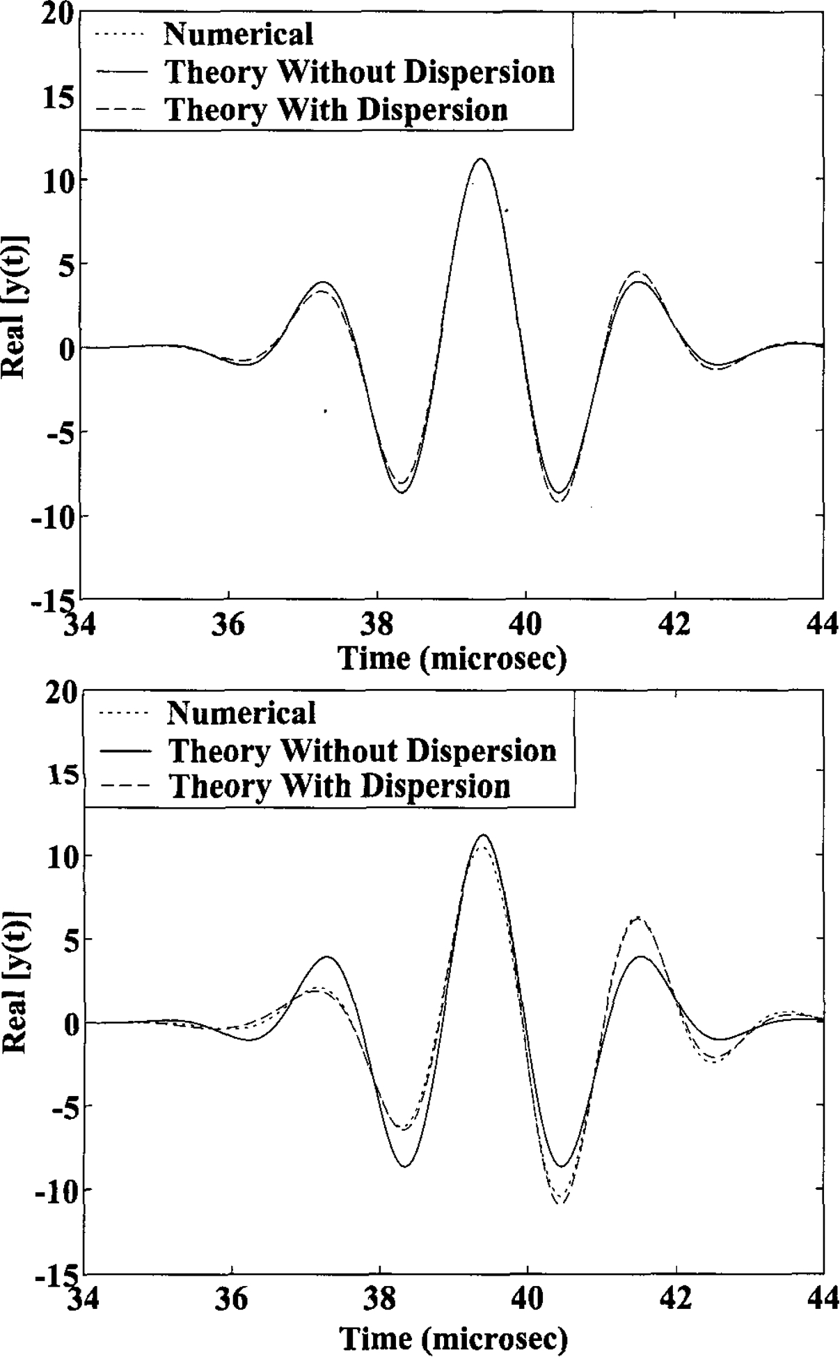
The relative importance of the dispersion-related errors in sound-speed estimates in bone. The three functions shown correspond to the received signal, y(t), obtained numerically without the assumption of weak dispersion (dotted line), analytically including dispersion effects (Equation 18, dashed line), and analytically ignoring dispersion effects (Equation 18 with g=0, solid line). The parameters used were typical for clinical bone sonometry (f₀=500 kHz, σ_f=100 kHz, β=2.3 cm⁻¹MHz⁻¹ or 20 dB/cmMHz, d=2 cm, and c_s=1550 cm/s at 500 kHz). In Figure 2a, b_s was taken from reported measurements in calcaneus to be −40 m/sMHz.³⁷ In this case, dispersion-related effects are negligible. In Figure 2b, an exaggerated value of b_s = −150 m/sMHz was assumed.

Comparing a two shifts from adjacent zero crossings, in the absence of dispersion effects,

$$s_{n+1}-s_n=\frac{1}{2}\left[\frac{1}{f_1}-\frac{1}{f_0}\right]$$ (27)

As one moves over one zero crossing in the direction from the leading edge toward the trailing edge of the pulse, the artifactual alteration in the location of the zero crossing shift increases. For media such as bone that have a faster sound speed than water, Δt is negative. This will cause the estimated speed of sound to decrease as the designated marker zero crossing for sound-speed determination is moved from the leading edge toward the trailing edge. For maxima or minima on the waveform, n may be approximated as a value equal to an integer plus one half.

Experimental Methods

Biological Methods

Twentyfour human calcaneus samples (both genders, ages unknown) were obtained. They were defatted using a trichloro-ethylene solution. Defatting was presumed not to significantly affect measurements since speed of sound of defatted trabecular bone has been measured to be only slightly different from that of bone with marrow left intact.^35,38 The cortical lateral layers were sliced off leaving two parallel surfaces with direct access to trabecular bone. The thicknesses of the samples varied from 12 to 21 mm. In order to remove air bubbles, the samples were vacuum degassed underwater in a desiccator. After vacuum, samples were allowed to thermally equilibrate to room temperature prior to ultrasonic interrogation. Ultrasonic measurements were performed in distilled water at room temperature. The temperature was measured for each experiment and ranged between 19.1°C and 21.2°C. The relative orientation between the ultrasound beam and the calcanei was the same as with in vivo measurements performed with commercial bone sonometers, in which sound propagates in the mediolateral (or lateromedial) direction.

Ultrasonic Methods

In order to draw a connection with this work to soft tissue applications, a tissue-mimicking phantom was interrogated in addition to the bone samples. The sound speed was 1540 m/s. The attenuation coefficient was 0.57 dB/cmMHz. The phantom had a thickness of 5 cm.

A Panametrics (Waltham, MA) 5800 pulser/receiver was used. Samples were interrogated in a water tank using pairs of coaxially aligned Panametrics 1” diameter, focussed, broadband transducers with center frequencies of 500 kHz (bone samples) and 2.25 MHz (tissue mimicking phantom). Received ultrasound signals were digitized (8 bit, 10 MHz for 500 kHz data, 25 MHz for 2.25 MHz data) using a LeCroy (Chestnut Ridge, NY) 9310C Dual 400 MHz oscilloscope and stored on computer (via GPIB) for off-line analysis.

The temperature-dependent speed of sound in distilled water, c_w, was used as the reference speed and is the given by⁴⁷

$$c_w=1402.9+4.835T-0.047016T^2+0.00012725T^3$$ (28)

where T is the temperature in degrees Celsius. Each arrival time was computed as follows. First, the digitized received pulse was bandpass filtered with brick-wall frequency domain bandpass filter with limits from 200 kHz to 600 kHz. Then the signal was envelope detected using a Hilbert transform. The n=0 zero crossing was the first zero crossing after the central lobe of the pulse. This is a consequence of Equation 25 and choosing that value for ϕ₀ that is most consistent with the data and falling within the principal value range, i. e. −π < ϕ₀ # π. Zero crossing numbers count up as one moves toward the trailing edge of the pulse and down as one moves toward the leading edge. (See Figure 3). Uncompensated sound speed estimates and estimates compensated using Equation 26, yielding true group velocity, were computed.

3.

Recorded reference pulse (solid line) and Gaussian model fit (dashed line). The numbering scheme for zero-crossings −2, −1, 0, and 1 is also indicated. See Equations 5 and 25.

Generally speaking, this substitution technique can exhibit appreciable error if the speed of sound differs substantially between the sample and the reference.⁴⁸ However, one study indicates that this diffraction-related error is negligible in calcaneus.⁴² Apparently, the speed of sound in calcaneus, approximately 1475 – 1650 m/s,⁴² is sufficiently close to that of distilled water at room temperature, 1487 m/s,⁴⁷ that diffraction-related errors may be ignored.

Results

Figure 3 illustrates the approximate Gaussian nature of the pulse used. The recorded reference pulse (solid line) and the Gaussian model fit (dashed line) are shown. Excellent agreement may be seen. The numbering scheme for zero-crossings −2, −1, 0, and 1 is also indicated.

Figure 4 shows speed of sound measurements in the phantom using zero crossings −2, −1, 0, and 1 as markers. The solid line shows uncompensated measurements (circles) and the dashed line (squares) shows measurements compensated using Equation 26. The progressive decline in sound-speed estimate as the marker is moved from the leading edge toward the trailing edge of the pulse is predicted by Equation 27. Error bars denote standard deviations. In this example, the magnitude of this variation is on the order of a few m/s and is not unacceptably large for most applications. (However, this variation can increase considerably as the attenuation coefficient and bandwidth increase. See Discussion Section.) Nevertheless, when measurements are compensated, the dependence of sound-speed estimates on marker location is removed. The small difference between the sound-speed measured here (1538 m/s) and the manufacturer-specified value (1540 m/s) may be attributable to temperature effects and/or differences in sound-speed computation algorithm.

4.

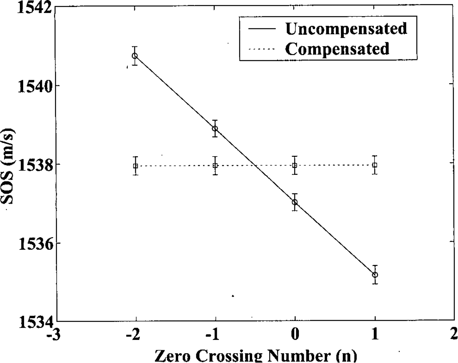
Speed of sound measurements in a phantom using zero crossings −2, −1, 0, and 1 as markers. The solid line shows uncompensated measurements (circles) and the dashed line (squares) shows measurements compensated using Equation 26. Error bars denote standard deviations.

Figure 5 shows average speed of sound measurements in the 24 bone samples using zero crossings −2, −1, 0, and 1 as markers. The solid line (circles) shows uncompensated measurements and the dashed line shows measurements (squares) compensated using Equation 26. Error bars denote standard errors. Also shown are measurements with a similar system (a pair of 500 kHz center frequency, broadband, 1.25” diameter, focused transducers) published by Laugier et al.³⁵ (who also used maxima and minima to estimate sound speed, resulting in non-integral values for n in the formalism used here) in a single bone specimen (x’s). Both sets of uncompensated measurements exhibit the same downward trend as one moves from the leading edge of the pulse toward the trailing edge predicted by Equation 27. Here, due to the high attenuation coefficient for bone and the corresponding high center frequency shift, the degree of variation among measurements is substantial and on the order of 40–50 m/s. Compensation, using equation 26 removes this variability. It may also be seen in Figure 5 that errors in group velocity estimates for uncompensated measurements are minimized when the zero crossing marker is chosen near the center of the waveform (n=0 or n=−1).

5.

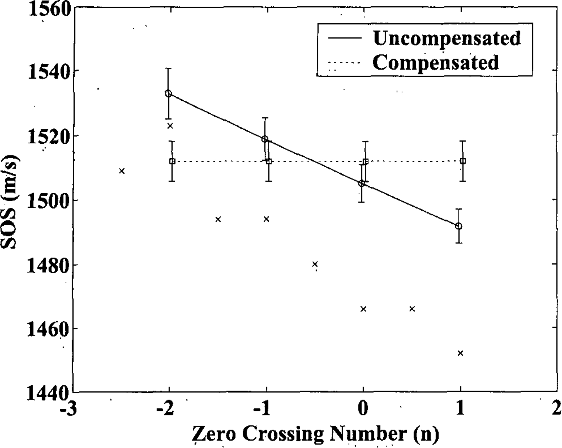
Average speed of sound measurements in the 24 bone samples using zero crossings −2, −1, 0, and 1 as markers. The solid line (circles) shows uncompensated measurements and the dashed line shows measurements (squares) compensated using Equation 26. Error bars denote standard errors. Also shown are similar measurements published by Laugier et al.³⁹ in a single bone specimen (x’s).

Discussion

Frequency-dependent attenuation and dispersion may alter the shape of a propagating ultrasound pulse, thereby introducing variations in time-domain, through-transmission, substitution-method-based sound-speed estimates. In this paper, theory has been presented for a correction for this distortion for Gaussian pulses propagating through linearly-attenuating, weakly-dispersive media. The theory has been validated using numerical analysis, measurements on a tissue mimicking phantom, and on 24 human calcaneus samples in vitro. Variations in soft-tissue-like media are generally not exceptionally large for most applications but can be substantial (see below), particularly for broad bandwidth pulses propagating through media with high attenuation coefficients. Using 500 kHz broadband transducers, typical for clinical bone sonometry, variations in velocity estimates in bone were found to be very substantial, on the order of 40–50 m/s, due to the high attenuation coefficient of bone. Dispersion-related variations, on the other hand, were found to be negligible in bone.

Since the magnitude of the sound speed estimate depends on the spectral properties of the pulse and the location of the particular marker chosen for arrival time determination, meaningful comparison of measurements performed with different systems using different algorithms can be difficult if not impossible. This is especially true since relatively subtle variations in sound speed can carry important diagnostic information. For example, in one important prospective study of 5662 elderly women,²⁴ baseline sound speed measurements were 1479.9 ± 23.8 m/s (mean ± standard deviation) for subjects who experienced a hip fracture over a subsequent two year period compared with 1493.4 ± 24.2 m/s for subjects who did not. The difference, 13.5 m/s, is small relative to differences that can occur due to different marker designations. It would be a great step toward standardization if manufacturers of bone sonometers employed the methodology described in this paper (or at least chose a marker as near as possible to the center of the pulse) in order to measure true group velocity and thereby minimize system dependence of sound-speed measurements.

The theory presented here predicts that, for media such as bone that have a faster sound speed than water, the estimated speed of sound decreases as the designated marker is moved from the leading edge toward the trailing edge of the pulse. This effect has been reported previously by Laugier et al.³⁹ and Nicholson et al.³⁷ and qualitatively attributed to spectral changes due to frequency-dependent attenuation and dispersion. Figure 6 illustrates the magnitude of this effect for the n=−2 zero crossing (which is only one half cycle away from the central lobe of the pulse) as a function of frequency shift, Δf = σ_f²βd, for a 2 cm thick calcaneus sample with sound speed equal to 1530 m/s, interrogated at 500 kHz. The arrow shows the frequency shift for a sample with attenuation coefficient of 20 dB/cmMHz, and the bandwidth measured for the experimental system used in this paper resulting in an error in group velocity estimates of about 20 m/s. Thicker samples, more highly attenuating samples, and/or higher bandwidth transducers would produce larger errors. Thicker samples would be expected to be encountered in vivo. Attenuation coefficients in calcaneus have been reported to range from 4 dB/cmMHz to 32 dB/cmMHz.⁴⁹

6.

Estimated velocity (if not compensated using Equation 26) for the n=−2 zero crossing (one half cycle prior to the central lobe of the pulse) as a function of frequency shift, Δf = σ_f²βd, for a typical 2 cm thick calcaneus sample with sound speed equal to 1530 m/s, interrogated at 500 kHz. The arrow shows the frequency shift for a sample with attenuation coefficient of 20 dB/cmMHz, and the bandwidth measured for the experimental system used in this paper resulting in an error of about 20 m/s.

Figure 7 illustrates the magnitude of the error in the group velocity estimate, as a function of frequency shift, for a 5 cm thick sample with sound speed equal to 1540 m/s, interrogated at 2.25 MHz. The arrow shows the frequency shift for a sample with attenuation coefficient of 0.57 dB/cmMHz (same as the phantom used in this experiment), and the bandwidth measured for the experimental system used in this paper resulting in an error of about 3 m/s. This level of accuracy is generally acceptable for most applications. However, thicker or more highly attenuating samples and/or higher bandwidth transducers would produce larger errors. Note in particular that bandwidth is generally linearly related to frequency and that frequency shift is quadratically related to bandwidth (see Equation 9). For example, it can be seen in Figure 7 that doubling the center frequency (and hence multiplying the frequency shift by approximately a factor of 4) would lead to errors on the order of 25 m/s.

7.

Estimated velocity (if not compensated using Equation 26) for the n=−2 zero crossing (one half cycle prior to the central lobe of the pulse) as a function of frequency shift, Δf = σ_f²βd, for a 5 cm thick sample with sound speed equal to 1540 m/s, interrogated at 2.25 MHz. The arrow shows the frequency shift for a sample with attenuation coefficient of 0.57 dB/cmMHz (same as the phantom used in this experiment), and the bandwidth measured for the experimental system used in this paper resulting in an error of about 3 m/s. See Discussion section for conditions under which errors become more significant.

Recently, an interlaboratory comparison of ultrasonic backscatter, attenuation, and speed measurements was conducted. In this study, phantoms were constructed at the University of Wisconsin and distributed to ten laboratories.⁵⁰ The laboratories independently performed measurements. (The phantom investigated in the present paper with sound speed of 1540 m/s and attenuation coefficient of 0.57 dB/cmMHz was one of the phantoms). The results were plotted collectively so that the various measurement techniques could be compared. Frequencies ranging from 2 MHz to 8 MHz were used. In general, the ten sets of investigators gave little or no detail regarding the location of the reference point on the pulse that was used in time-of-flight methods.⁵⁰ However, measurements reported by the various laboratories ranged from 1535 – 1553 m/s. It is plausible that the effects investigated in the present paper contributed substantially to this variation.

References

- 1.Duck FA. Physical properties of tissue. Cambridge, UK: University Press, 1990. [Google Scholar]
- 2.Dunn F, and Goss SA. “Definition of terms and measurement of acoustical quantities,” In: Greenleaf JF, ed. Tissue characterization with ultrasound. Boca Raton, FL: CRC Press, 1986:15–55. [Google Scholar]
- 3.Goss SA, Johnston RL, and Dunn F. “Comprehensive compilation of empirical ultrasonic properties of mammalian tissues.” J. Acoust. Soc. Am, 64, 423–457, 1978. [DOI] [PubMed] [Google Scholar]
- 4.Bamber JC, Speed of Sound. In Hill CR, ed. Physical principles of medical ultrasonics. Chichester, UK: Ellis Horwood, 1986:200–224. [Google Scholar]
- 5.Wells PNT, Biomedical Ultrasonics. London, UK: Academic Press. 1977. [Google Scholar]
- 6.Wladimiroff JW, Craft LL, and Talbert DG. “In vitro measurements of sound velocity in human fetal brain tissue.” J. Obset. Gyn. Brit. Comm 71, 11–20, 1975. [DOI] [PubMed] [Google Scholar]
- 7.Kremkau FW, Barnes RW, and McGraw CP. “Ultrasonic attenuation and propagation speed in normal human brain.” J. Acoust. Soc. Am, 70, 29–38, 1981. [Google Scholar]
- 8.Sehgal CM, Brown GM, Bahn RC, and Greenleaf JF. “Measurement and use of acoustic nonlinearity and sound speed to estimate composition of excised livers.” Ultrason. Med. & Biol, 12, 865–874, 1986. [DOI] [PubMed] [Google Scholar]
- 9.Bamber JC and Hill CR. “Acoustic properties of normal and cancerous human liver – I. Dependence on pathological condition.” Ultrason. Med. & Biol, 7, 121–133, 1981. [DOI] [PubMed] [Google Scholar]
- 10.Tervola KMU, Gummer MA, Erdman JW, and O’Brien WD. “Ultrasonic attenuation and velocity properties in rat liver as a function of fat concentration: a study at 100 MHz using a scanning laser acoustic microscope.” J. Acoust. Soc. Am, 77, 307–313, 1985. [DOI] [PubMed] [Google Scholar]
- 11.O’Brien WD, Erdman JW, and Hebner TB. “Ultrasonic propagation properties (@ 100 MHz) in excessively fatty rat liver.” J. Acoust. Soc. Am, 83, 1159–1166, 1988. [DOI] [PubMed] [Google Scholar]
- 12.O’Brien WD. “The relationship between collagen and ultrasonic attenuation and velocity in tissue.” Ultrasonic International 1977, 194–205, 1977. [Google Scholar]
- 13.Rooney JA, Gammel PM, Hestenes JD, Chin HP, and Blankenhorn DH. “Velocity and attenuation of sound in arterial tissues.” J. Acoust. Soc. Am, 71, 462–466, 1982. [DOI] [PubMed] [Google Scholar]
- 14.Olerud JE, O’Brien WD, Reiderer-Henderson MA, Steiger DL, Debel JR, and Odland GF. “Correlation of tissue constituents with the acoustic properties of skin and wound.” Ultrason. Med. & Biol, 16, 55–64, 1990. [DOI] [PubMed] [Google Scholar]
- 15.Rossman P, Zagzebski J, Mesina C, Sorenson J, and Mazess R, “Comparison of Speed of Sound and Ultrasound Attenuation in the Os Calcis to Bone Density of the Radius, Femur and Lumbar Spine,” Clin. Phys. Physiol.Meas, 1989; 10:353–360. [DOI] [PubMed] [Google Scholar]
- 16.Tavakoli MB and Evans JA. “Dependence of the velocity and attenuation of ultrasound in bone on the mineral content.” Phys. Med. Biol, 36, 1529–1537, (1991). [DOI] [PubMed] [Google Scholar]
- 17.Zagzebski JA, Rossman PJ, Mesina C, Mazess RB, and Madsen EL. “Ultrasound transmission measurements through the os calcis.” Calcif Tissue Int. 49, 107–111, 1991. [DOI] [PubMed] [Google Scholar]
- 18.Njeh CF, Hodgskinson R, Currey JD, and Langton CM. “Orthogonal relationships between ultrasonic velocity and material properties of bovine cancellous bone.” Med. Eng. Phys, 18, 373–381, 1996. [DOI] [PubMed] [Google Scholar]
- 19.Laugier P, Droin P, Laval-Jeantet AM, and Berger G. “In vitro assessment of the relationship between acoustic properties and bone mass density of the calcaneus by comparison of ultrasound parametric imaging and quantitative computed tomography.” Bone, 20, 157–165, 1997. [DOI] [PubMed] [Google Scholar]
- 20.Nicholson PHF, Muller R, Lowet G, Cheng XG, Hildebrand T, Ruegsegger P, Van Der Perre G, Dequeker J, and Boonen S. “Do quantitative ultrasound measurements reflect structure independently of density in human vertebral cancellous bone?” Bone. 23, 425–431, 1998. [DOI] [PubMed] [Google Scholar]
- 21.Hans D, Wu C, Njeh CF, Zhao S, Augat P, Newitt D, Link T, Lu Y, Majumdar S, and Genant HK. “Ultasound velocity of trabecular cubes reflects mainly bone density and elasticity.” Calcif. Tissue Intl 64, 18–23, 1999. [DOI] [PubMed] [Google Scholar]
- 22.Trebacz H, and Natali A. “Ultrasound velocity and attenuation in cancellous bone samples from lumbar vertebra and calcaneus.” Osteo. Int’l, 9, 99–105, 1999. [DOI] [PubMed] [Google Scholar]
- 23.Cummings SR, Black DM, Nevitt MC, Browner W, Cauley J, Ensrud K, Genant HK, Palermo L, Scott J, and Vogt TM. “Bone density at various sites for prediction of hip fractures.” Lancet, 341, 72–75, 1993. [DOI] [PubMed] [Google Scholar]
- 24.Hans D, Dargent-Molina P, Schott AM, Sebert JL, Cormier C, Kotzki PO, Delmas PD, Pouilles JM, Breart G, and Meunier PJ. “Ultrasonographic heel measurements to predict hip fracture in elderly women: the EPIDOS prospective study,” Lancet, 348, 511–514, 1996. [DOI] [PubMed] [Google Scholar]
- 25.Bauer DC, Gluer CC, Cauley JA, Vogt TM, Ensrud KE, Genant HK, and Black DM. “Broadband ultrasound attenuation predicts fractures strongly and independently of densitometry in older women,” Arch. Intern, Med 157, 629–634 1997. [PubMed] [Google Scholar]
- 26.Schott AM, Weill-Engerer S, Hans D, Duboeuf F, Delmas PD, and Meunier PJ, “Ultrasound discriminates patients with hip fracture equally well as dual energy X-ray absorptiometry and independently of bone mineral density.” J. Bone Min. Res, 10, 243–249 1995. [DOI] [PubMed] [Google Scholar]
- 27.Turner CH, Peacock M, Timmerman L, Neal JM, and Johnston CC Jr., “Calcaneal ultrasonic measurements discriminate hip fracture independently of bone mass,” Osteo. International, 5, 130–135 1995. [DOI] [PubMed] [Google Scholar]
- 28.Glüer CC, Cummings SR, Bauer DC, Stone K, Pressman A, Mathur A, and Genant HK. “Osteoporosis: Association of recent fractures with quantitative US findings”, Radiology, 199, 725–732 1996. [DOI] [PubMed] [Google Scholar]
- 29.Thompson P, Taylor J, Fisher A, and Oliver R, “Quantitative heel ultrasound in 3180 women between 45 and 75 years of age: compliance, normal ranges and relationship to fracture history,” Osteo. Int’l, 8, 211–214, 1998. [DOI] [PubMed] [Google Scholar]
- 30.Lees S, Cleary PF, Heeley JD, and Gariepy EL. “Distribution of sonic plesio-velocity in a compact bone sample.” J. Acoust. Soc. Am, 66, 641–646, 1979 [Google Scholar]
- 31.Lakes R, Yoon HS, and Katz JL, “Slow compressional wave propagation in wet human and bovine cortical bone”, Science, 220, 513–515, 1983. [DOI] [PubMed] [Google Scholar]
- 32.Lakes R, Yoon HS, and Katz JL, “Ultrasonic wave propagation and attenuation in wet bone.” J. Biomed. Eng, 8, 143–148, 1986. [DOI] [PubMed] [Google Scholar]
- 33.Lees S and Klopholz DZ, “Sonic velocity and attenuation in wet compact cow femur for the frequency range 5 to 100 MHz.” Ultrasound in Med. & Biol, 18, 303–308, 1992. [DOI] [PubMed] [Google Scholar]
- 34.Morse PM and Ingard KU. Theoretical Acoustics. Princeton, NJ: Princeton University Press, 1968, Chapter 9. [Google Scholar]
- 35.Njeh CF and Langton CM. “The effect of cortical endplates on ultrasound velocity through the calcaneus: an in vitro study.” Brit. J. Radiol, 70, 504–510, 1997. [DOI] [PubMed] [Google Scholar]
- 36.Njeh CF, Kuo CW, Langton CM, Atrah HI, and Boivin CM. “Prediction of human femoral bone strength using ultrasound velocity and BMD: an in vitro study.” Osteo. Int’l 7, 471–477, 1997. [DOI] [PubMed] [Google Scholar]
- 37.Nicholson PHF, Lowet CG, Langton CM, Dequeker J, and Van der Perre G, “Comparison of time-domain and frequency-domain approaches to ultrasonic velocity measurements in trabecular bone,” Phys. Med. Biol, 41, 2421–2435, 1996. [DOI] [PubMed] [Google Scholar]
- 38.Alves JM, Xu W, Lin D, Siffert RS, Ryaby JT, and Kaufmann JJ. “Ultrasonic assessment of human and bovine trabecular bone: a comparison study.” IEEE Trans. Biomed. Eng 43, 249–258. [DOI] [PubMed] [Google Scholar]
- 39.Laugier P, Giat P, Droin P,P, Saied A, and Berger G. “Ultrasound images of the os calcis: a new method of assessment of bone status.” Proc. IEEE Ultrasonics Symp., Sponsor: Ultrasonics Ferroelectric & Frequency Control Soc, 31 Oct.–3 Nov. 1993, Baltimore, MD, USA vol.2 , Page: 989–92, Editor: Levy M; McAvoy BR Publisher: IEEE, New York, NY, USA, 1993. [Google Scholar]
- 40.Zagzebski JA, Rossman PJ, Mesina C, Mazess RB, and Madsen EL, “Ultrasound transmission measurements through the os calcis,” Calcif. Tissue Int’l, 49, 107–111, 1991. [DOI] [PubMed] [Google Scholar]
- 41.Strelitzki R, and Evans JA, “On the measurement of the velocity of ultrasound in the os calcis using short pulses,” Eur. J. Ultrasound, 4, pp. 205–213, 1996. [Google Scholar]
- 42.Droin P, Berger G, and Laugier P. “Velocity dispersion of acoustic waves in cancellous bone.” IEEE Trans. Ultrason. Ferro. Freq. Cont 45, 581–592, 1998. [DOI] [PubMed] [Google Scholar]
- 43.Ragozzino M. “Analysis of the error in measurement of ultrasound speed in tissue due to waveform deformation by frequency-dependent attenuation.” Ultrasonics, 19, 135–138, 1981. [DOI] [PubMed] [Google Scholar]
- 44.Narayana PA and Ophir J, “A closed form method for the measurement of attenuation in nonlinearly dispersive media,” Ultrason. Imag, 5, 17–21, 1983. [DOI] [PubMed] [Google Scholar]
- 45.O’Donnell M, Jaynes ET, and Miller JG, “Kramers-Kronig relationship between ultrasonic attenuation and phase velocity.” J. Acoust. Soc. Am, 69, 696–701, 1981. [Google Scholar]
- 46.Bracewell RN. The Fourier Transform and Its Applications. New York, NY: McGraw-Hill, 1978. [Google Scholar]
- 47.Kaye GWC, and Laby TH. Table of Physical and Chemical Constants. London, UK: Longman, 1973. [Google Scholar]
- 48.Kaufman JJ, Xu W, Chiabrera AE, and Siffert RS, “Diffraction effects in insertion mode estimation of ultrasonic group velocity,” IEEE Trans. Ultrason. Ferroelectr. Freq. Contr, 42, 232–242, 1995. [Google Scholar]
- 49.Langton CM, Njeh CF, Hodgskinson R, and Currey JD. “Prediction of Mechanical Properties of the Human Calcaneus by Broadband Ultrasonic Attenuation,” Bone, 18, 495–503, (1996). [DOI] [PubMed] [Google Scholar]
- 50.Madsen EL, Dong F, Frank GR, Garra BS, Wear KA, Wilson T, Zagzebski JA, Miller HL, Shung KK, Wang SH, Feleppa EJ, Liu T, O’Brien WD, Topp KA, Sanghvi NT, Zaitseo AV, Hall TJ, Fowlkes HB, Kripfgans OD, and Miller JG, “Interlaboratory comparison of ultrasonic backscatter, attenuation and speed measurements.” J. Ultrason. Med 18, 615–632, 1999. [DOI] [PubMed] [Google Scholar]