Have paved trails and protected bike lanes led to more bicycling in Atlanta? A generalized synthetic-control analysis

Abstract

Background:

Bicycling is an important form of physical activity in populations. Research assessing the effect of infrastructure on bicycling with high-resolution smartphone data is emerging in several places, but it remains limited in low-bicycling U.S. settings, including the Southeastern U.S. The Atlanta area has been expanding its bicycle infrastructure, including off-street paved trails such as the Atlanta BeltLine and some protected bike lanes.

Methods:

Using the generalized synthetic control method, we estimated effects of five groups of off-street paved trails and protected bike lanes on bicycle ridership in their corresponding areas. To measure bicycling, we used 2 years (2016–10-01 to 2018–09-30) of monthly Strava data in Atlanta’s urban core along with data from 15 on-the-ground counters to adjust for spatiotemporal variation in app use.

Results:

Considering all infrastructure as one joint intervention, an estimated 1.10 (95% confidence interval [CI]: 0.99, 1.18) times more bicycle–distance was ridden than would have been expected in the same areas had the infrastructure not been built, when defining treatment areas by the narrower of two definitions (defined in text). The Atlanta BeltLine Westside Trail and Proctor Creek Greenway had especially strong effect estimates, e.g., ratios of 1.45 (95% CI: 1.12, 1.86) and 1.55 (1.10, 2.14) under each treatment-area definition, respectively. We estimated that other infrastructure had weaker positive or no effects on bicycle–distance ridden.

Conclusions:

This study advances research on the topic because of its setting in the U.S. Southeast, simultaneous assessment of several infrastructure groups, and data-driven approach to estimating effects.

INTRODUCTION

Physical inactivity is a global public-health problem.¹ Promoting bicycling is a well-recognized public-health strategy to combat this pandemic.² In the U.S., a Healthy People 2030 objective is to “increase the proportion of adults who walk or use a bicycle to get to and from places.”³ Bicycling is appealing from a public-health perspective² because it is inexpensive and can serve as transportation, possibly replacing sedentary and greenhouse-gas-emitting travel with physical activity. Bicycling levels in the U.S. are low compared with other wealthy nations;⁴ the proportion of commuters who bicycle to work is less than 1%.⁵ Given the low levels of bicycling in the U.S., increasing bicycling represents a public-health opportunity.

In most settings, collective health benefits of bicycling are assumed to outweigh risks (e.g., injury or pollution exposure).^6,7 Still, bicycling levels are low in the U.S. partly due to the understandable concern that it is unsafe.^5,8–10 Creating more welcoming built environments for non-motorized travel is a key part of U.S. public-health strategy to promote bicycling.^11,12 The National Physical Activity Plan, for example, includes a section on transportation and community design. Authors endorsing the plan have asserted that increasing population levels of physical activity “…will require altering the physical and social environments in which Americans work, play, learn, and travel.”¹¹

While data suggest bicycle-specific infrastructure, such as off-street paved trails and protected bicycle lanes, can induce bicycling,¹³ existing built-environment literature has limitations.^14,15 Some research on the topic has used cross-sectional surveys,¹³ making it difficult to rule out reverse causality. Longitudinal studies exist, but until recently, have included few time points with limited spatial coverage.^16–19 Bicycling data with rich spatiotemporal detail as measured with a smartphone app have become more commonly used in descriptive research.^20,21 Etiologic research assessing the effect of infrastructure on bicycling with this type of data has emerged in some countries,^16–18 but research using objective measures in low-bicycling U.S. settings is limited.^19,22–24

One such low-bicycling region is the Southeastern U.S. Eight of the ten U.S. states with the lowest bicycling-to-work estimates are in the Southeast.⁵ Some Southeast municipalities have sought to change these figures.⁵ Atlanta, Georgia, known for its car-oriented built environment,^25,26 has been expanding its bicycling infrastructure.

Part of this new infrastructure is the Atlanta BeltLine,^26–29 a project converting a 22-mile former railroad corridor into off-street paved trails for walking, bicycling, and transit. Including spur trails, a total of 33 miles of BeltLine trail are planned, 14 of which were completed by the end of 2017.²⁸ Encircling Atlanta’s urban core, the BeltLine connects neighborhoods that have been historically racially segregated.^26,30 Against a national context of inequitable access to health-promoting built environments,³¹ the project has the potential to address health equity³² and improve access to healthy built environments for historically oppressed communities in Atlanta, although housing affordability is a concern.²⁷ Other recently constructed paved trails and lanes include the Proctor Creek Greenway on Atlanta’s northwest side; the PATH Parkway and Luckie Street protected bike lane, which together link Georgia Institute of Technology with downtown; and the South Peachtree Creek Trail in North Decatur. The amount and diversity of this infrastructure presents an opportunity for evaluation.

In this study, we estimate effects of the installation of off-street paved trails and protected bike lanes in Atlanta, Georgia on bicycle ridership in the nearby area. To do so, we use spatially detailed longitudinal bicycling data generated from a smartphone app combined with data from stationary counters to adjust for place-and-time-varying trends in app use.

METHODS

Study setting

Atlanta, Georgia, is a city of about 500,000 people and about 6 million in the metro area with a mild winter climate. Per the American Community Survey, an estimated 0.8% of Atlantans commute by bicycle, whereas about two thirds of commuters drive to work alone. Our study took place over a 24-month period, 2016–10-01 to 2018–09-30, in roughly a 6-mile radius around the intersection of Ponce de Leon Ave NE and Monroe Dr NE (Figure 1).

Figure 1.

The treatment infrastructure and corresponding wide-net (A) and narrower (B) definition of the treatment areas. The total number of hexagons treated varies over time under each definition (Figure 2); these maps represent the last study month (September 2018). Abbreviations: WST-PCG, Atlanta BeltLine Westside Trail & Proctor Creek Greenway; LS-TECH-IAP, Luckie Street NW Protected Bike Lane & Georgia Tech PATH Parkway & Ivan Allen PATH; EST-EXT, Atlanta BeltLine Eastside Trail Extension; MCD, North McDonough St Protected Bike Lane; NT, never treated. Abbreviations for each section of treatment infrastructure are defined in Table 1.

Treatment: the bicycle infrastructure

The infrastructure

We evaluated off-street paved trails and protected bike lanes that opened in 2017 and 2018. Off-street paved trails are physically separated from roadways and are designed for use by bicyclists, pedestrians, or other light individual transportation.³³ They typically do not follow the road network. Protected bike lanes, also called cycle-tracks, use a curb-like barrier, parked cars, or delineator posts to physically separate bicyclists from motorized traffic. Protected bike lanes are directly adjacent to the roadway and differ from conventional bike lanes by having a physical barrier; conventional lanes only use paint.

Specifically, we studied five groups of bicycling infrastructure, which opened at varying times (Table 1; Figure 1): 1) the Atlanta BeltLine Westside Trail and Proctor Creek Greenway; 2) the PATH Parkway Trail, a protected bike lane along Luckie Street NW, and the Ivan Allen PATH; 3) extensions of the Atlanta Beltline Eastside Trail; 4) sections of the South Peachtree Creek Trail; and 5) a protected bike lane on North McDonough Street. Table 1 has more description.

Table 1.

The groups of bicycle infrastructure evaluated, sorted from west to east.

Treatment infrastructure group name (abbreviation)	Treatment infrastructure section name (abbreviation)	Type	Neighborhood	Length (mi)	Date opened	For further information
Atlanta BeltLine Westside Traila & Proctor Creek Greenway (WST-PCG)	Atlanta BeltLine Westside Trail (WST)	Off-street paved trail	Adair Park to Washington Park	2.41	2017–09-29	Atlanta Beltline 2017 Annual Report, p. 2569; City of Atlanta 2017 Annual Bicycle Report, p. 728
	Proctor Creek Greenway (PCG)	Off-street paved trail	Bankhead / Grove Park	2.45	2018–05-07	Atlanta Beltline 2018 Annual Report, p. 3168; City of Atlanta 2018 Annual Bicycle Report, p. 1629
Luckie St & PATH Parkway & Ivan Allen PATHb (LS-TECH-IAP)	Luckie St NW (LS)b	Protected bike lane	Downtown Atlanta	0.82	2017–06-01	Kahn, 201770
	Georgia Tech PATH Parkway (TECH)b	Off-street paved trail	Marietta St Artery / Georgia Tech	0.65	2017–11-28	City of Atlanta 2017 Annual Bicycle Report, p. 828; PATH Foundation71
	Ivan Allen PATH (IAP)	Off-street paved trail	Downtown / Vine City	0.66	2018–02-01	City of Atlanta 2018 Annual Bicycle Report, p. 1529
Atlanta BeltLine Eastside Extension (EST-EXT)	Atlanta BeltLine Eastside Trail: Krog St. NE to BeltLine corridor via Wylie St SE (EST-EXT1)	Off-street paved trail	Reynoldstown	0.36	2017–09-01	Atlanta Beltline 2017 Annual Report, p. 2969; Atlanta Beltline 2018 Annual Report, p. 2868
	Atlanta BeltLine Eastside Trail: Irwin St NE to Edgewood Ave NE (EST-EXT 2)	Off-street paved trail	Inman Park	0.23	2017–10-23
	Atlanta BeltLine Eastside Trail: Wylie St SE to Kirkwood Ave SE via BeltLine corridor (EST-EXT3)	Off-street paved trail	Reynoldstown	0.16	2017–10-23
South Peachtree Creek Trail (PCT)	South Peachtree Creek Trail: Mason Mill Park to N. Druid Hills Rd. (PCT1)	Off-street paved trail	North Decatur	0.87	2017–06-24	Williams, 201772; 201873
	South Peachtree Creek Trail: Starvine Way to Clairmont Road underpass (PCT2)	Off-street paved trail	North Decatur	0.22	2018–04-20
North McDonough St (MCD)	North McDonough St (MCD)	Protected bike lane	Downton Decatur	0.25	2017–09-01	Banks, 201774

^aThe length does not include the unpaved part in the corridor between Lawton St SW. and Ralph David Abernathy Blvd SW.

^bBetween Merrits Ave NW and North Ave NW, this protected bike lane is entirely off the street and could be called an off-street paved trail along that stretch. Conversely, because the PATH Parkway runs adjacent and parallel to a street (Tech Parkway NW), it could be called a protected bike lane rather than off-street paved trail.

Defining the treated and untreated areas over time

To define areas and time periods as treated with the infrastructure, we first divided the study area into hexagons³⁴ (n=298) of 0.5 square miles (Figure 1) for each study month (n=24). The hexagon–month (n=7,152) was our unit of analysis. We sub-divided the study area into hexagons of equal size because the generalized synthetic control method (described below) requires a consistent unit for both treated and untreated areas over time.

We then considered two treatment definitions, varying the number of hexagon–months classified as treated. Under the first (“wide-net”) definition, we drew half-mile radial buffers around each section of infrastructure if it had been open for at least half of that month. We classified hexagon–months as treated if at least 5% of the hexagon’s area overlapped the infrastructure’s radial buffer in that month. Otherwise, the hexagon–month was classified as untreated. This definition created treatment areas of about 3.1 square miles per mile of trail or lane (measuring at the end of the study; Table 2). These areas are about the size of a one-mile radial buffer—a 1-mile buffer around a 2-mile straight line is 3.6 square miles per mile—which has previously been used to define bicycling environments.³⁵ Figure 1 (panel A) maps this treatment definition, and Figure 2 (panel A) illustrates the time-varying nature of the treatment; as more infrastructure opened, more hexagon–months were classified as treated.

Table 2.

Characteristics of the treated and never-treated areas^a based on the “wide-net” definition during the pre-treatment period (2016–10-01 – 2017-05–31).

Attribute	WST-PCG	LS-TECH-IAP	EST-EXT	PCT	MCD	Never treated (NT)
Size of treatment area (square miles) at study end (2018–09-30)	13.0	4.5	4.0	4.5	2.0	121.0
Combined length of treatment trail(s) or lane(s) (miles)	4.86	2.12	0.75	1.09	0.25	N/A
Treatment area (square miles) per mile at study end (2018–09-30)	2.7	2.1	5.4	4.1	7.9	N/A
Socio-demographic characteristicsb (Estimate (95% CI))
Population density (residents per square mile)	3,709 (3,552; 3,865)	8,763 (8,414; 9,132)	7,816 (7,560; 8,049)	3,590 (3,447; 3,735)	5,584 (5,341; 5,823)	3,876 (3,832; 3,920)
Median age of residents	35 (34; 36)	28 (27; 28)	32 (31; 32)	36 (34; 38)	36 (33; 39)	36 (36; 36)
Percent of residents Black	85% (78%; 86%)	36% (33%; 39%)	31% (28%; 35%)	12% (10%; 15%)	21% (17%; 25%)	37% (35%; 37%)
Percent of residents white	11% (10%; 13%)	45% (41%; 48%)	60% (57%; 64%)	69% (65%; 74%)	69% (64%; 75%)	53% (52%; 54%)
Percent of residents another race	4% (4%; 11%)	20% (15%; 25%)	8% (5%; 14%)	18% (13%; 23%)	10% (5%; 17%)	10% (10%; 13%)
Median household income (USD)	35,931 (33,089; 38,931)	56,152 (50,848; 61,013)	75,226 (69,505; 80,950)	75,958 (69,360; 82,552)	104,042 (91,434; 116,547)	80,172 (77,784; 82,226)
Median home value (USD)	145,162 (132,506; 158,925)	186,993 (169,875; 203,343)	370,264 (352,971; 389,546)	367,158 (341,490; 392,282)	523,799 (494,030; 553,814)	363,539 (356,025; 371,826)
Percent of residents who bicycle to work	0.6% (0.6%; 1.6%)	1.9% (1.4%; 2.8%)	3.2% (2.3%; 4.3%)	1.5% (0.9%; 2.3%)	3.0% (1.7%; 4.7%)	0.7% (0.7%; 1.5%)
Built-environment characteristics
Bicycle infrastructure (miles per square mile) (Mean (SD))c
Off-street paved trails	0.51 (0)	0.71 (0)	2.01 (0)	0.42 (0)	0.83 (0)	0.36 (0.003)
Protected bike lanes	0.02 (0)	0.31 (0)	0.04 (0)	0.00 (0)	0.00 (0)	0.01 (0)
Buffered bike lanes	0.02 (0)	0.10 (0)	0.11 (0)	0.00 (0)	0.00 (0)	0.01 (0)
Conventional bike lanes	0.59 (0)	2.49 (0)	1.09 (0)	0.00 (0)	0.50 (0)	0.37 (0)
Street density (miles of roadway per square mile)d	15	20	22	13	19	13
Bicycle-distance measures
Estimated (IPSW) bicycle-distance ridden (person-miles) per square mile per month (Mean (95% CI))	2,549 (2,436; 2,654)	23,185 (22,514; 23,730)	50,717 (48,727; 53,038)	8,030 (7,792; 8,286)	20,860 (20,115; 21,746)	7,268 (7,152; 7,392)
Strava-reported bicycle-distance (person-miles) per square mile per month (Mean (95% CI))	166	1,312	3,037	488	1,880	576
Estimated sampling fraction per month (Strava-reported person-miles/IPSW person-miles) (Estimate (95% CI))	6.5% (6.3%; 6.8%)	5.7% (5.5%; 5.8%)	6.0% (5.7%; 6.2%)	6.1% (5.9%; 6.3%)	9.0% (8.6%; 9.3%)	7.9% (7.8%; 8.1%)

^aAlthough this table characterizes the areas during the pre-treatment period (2016–10-01 – 2017-05–31), the areas themselves correspond to the land area as classified at the end of the study, as depicted in Figure 1, panel A.

^bA weighted average of census-tract-level data from the 2015–2019 5-year American Community Survey (ACS; eAppendix 2). These measures are considered time-invariant over the study period.

^cMean and SD describe monthly variation during the pre-treatment period (2016–10-01 – 2017-05–31).

^dExcluding interstate highways, unclassified roads, and service roads, per the OpenStreetMap definition.⁷⁵ Street connectivity is considered time-invariant, so a standard deviation is not presented.

Abbreviations: Abbreviations: WST-PCG, Atlanta BeltLine Westside Trail & Proctor Creek Greenway; LS-TECH-IAP, Luckie Street NW Protected Bike Lane & Georgia Tech PATH Parkway & Ivan Allen PATH; EST-EXT, Atlanta BeltLine Eastside Trail Extension; MCD, North McDonough St Protected Bike Lane, NT, never treated; CI, confidence interval; IPSW, inverse-probability-of-selection weighted; SD, standard deviation.

Figure 2.

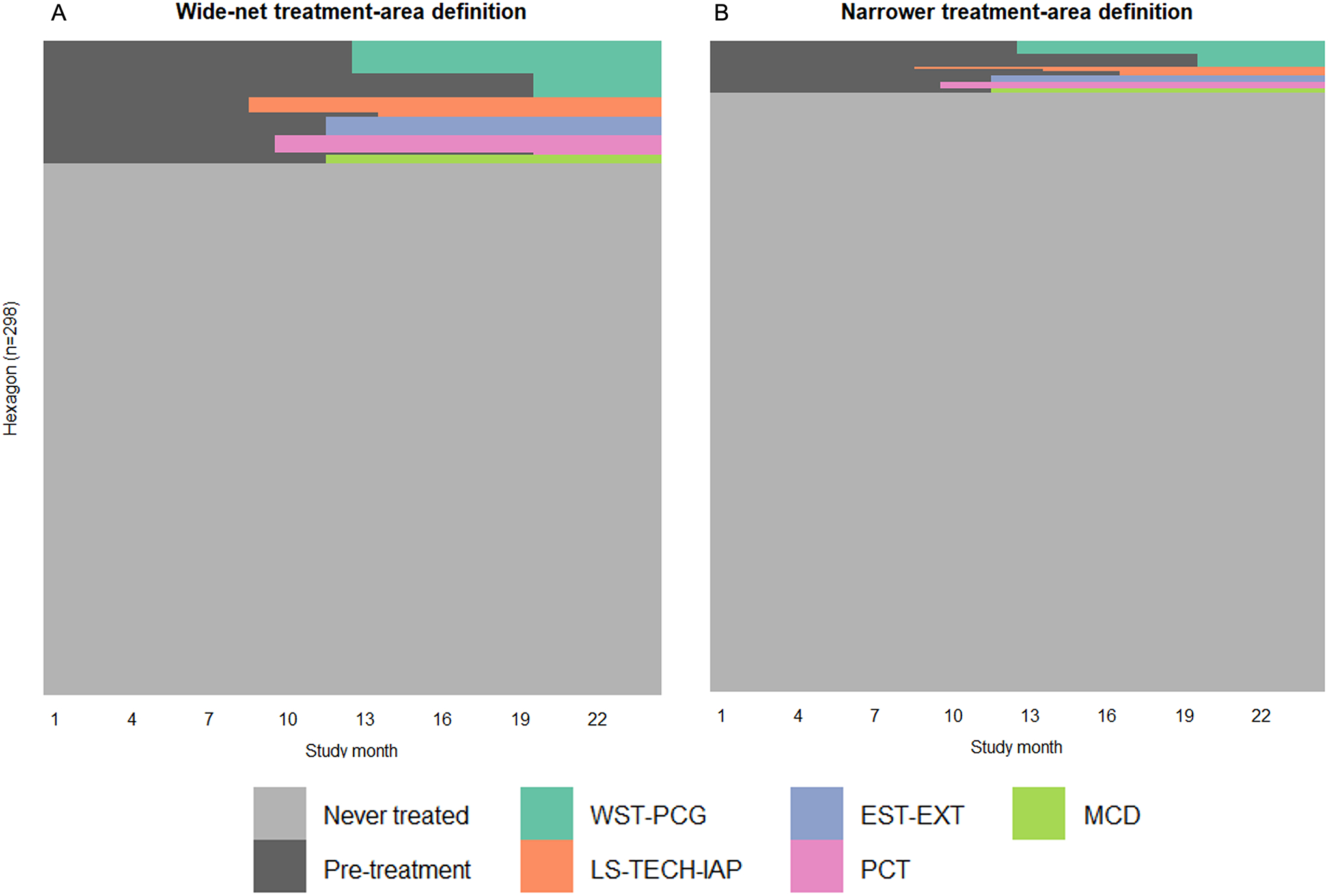
The treatment status of each hexagon-month (N=298 hexagons*24 months=7,172 hexagon-months) under each treatment-area definition, wide-net (A) or narrower (B). Abbreviations: WST-PCG, Atlanta BeltLine Westside Trail & Proctor Creek Greenway; LS-TECH-IAP, Luckie Street NW Protected Bike Lane & Georgia Tech PATH Parkway & Ivan Allen PATH; EST-EXT, Atlanta BeltLine Eastside Trail Extension; MCD, North McDonough St Protected Bike Lane.

We expected this definition would have high sensitivity in that of all bicycle ridership in the study (all 7,152 hexagon–months) that was truly caused by the infrastructure (i.e., bicycle–distance ridden that would not have occurred or would have been shorter if not for the infrastructure), a large share of it would likely have passed through its wide-net treatment area. On the other hand, this definition may have low specificity in that it may poorly rule out ridership in the study area unaffected by the infrastructure. (We use sensitivity and specificity loosely; in eAppendix 1, we define our use of these terms in this context in a potential-outcome framework.) A related concern with the wide-net treatment area is spillover effects or interference³⁶ between treatment areas, given their proximity to one another (Figure 1). We thus considered a second, narrower treatment definition which we expected would have lower sensitivity but higher specificity. Under this definition, we classified hexagon–months as treated only if the trail or lane itself (rather than a buffer) intersected the hexagon during the infrastructure’s open months (Figures 1 and 2, Panel B).

Description of the treatment areas before treatment: socio-demographic and built-environment characteristics

For descriptive purposes, in Table 2, we present the distribution of residential socio-demographic characteristics, reported bicycling to work, street density, and pre-existing bicycle infrastructure for the wide-net treatment-areas. We estimated hexagon-level descriptive measures by weighting census-tract-level estimates from 2015–2019 American Community Survey (ACS) 5-Year Data (eAppendix 2). The racial and socioeconomic composition of the treatment areas vary considerably. In the area around the Westside Trail and Proctor Creek Greenway, an estimated 85% of residents were Black, compared with 13% of residents in the South Peachtree Creek Trail area, reflecting Atlanta’s racial segregation.³⁷ The pre-existing built environments also differed. The Eastside Trail Extension area, for example, had comparatively high density of streets (21.8 miles of roadway per square mile) and pre-existing off-street paved trails (2.01 miles per square mile). eTable2.1 presents analogous information for the narrower treatment-area definition. eAppendix 2 contains maps visualizing some of these measures.

Outcome: bicycle distance

Bicycling data sources: Strava and stationary counters (ZELT)

Our outcome of interest is area-level bicycle ridership, operationalized as the cumulative bicycle–distance ridden in a hexagon–month. Bicycle–distance (e.g., as measured in bicycle-miles) is a common measure of bicycle ridership.³⁸ To compute this area-level measure, we began with bicycling data from two data sources at the level of the segment–month. A segment (N=84,805 within the study area) is a unique stretch of roadway or trail. The main data source was Strava, a GPS-based mobile application some people use to record their bike rides. Data included 307,205 rides contributed by approximately 10,000 unique people over the study period and area. To protect user privacy, data were summarized by segment rather than by individual. Strava reports the number of times, n_i,j, a segment i was ridden upon in either direction in month j by a bicyclist using Strava on that ride.

Strava data constitute a subset of all bicycle ridership: not everyone who bicycles uses the app, those who do may not on every ride, and users and their use may change over time.^39–41 Although Strava often correlates highly with on-the-ground bicycle counts in urban areas,^20,21 previous research in Atlanta suggested that Strava users are disproportionately enthusiastic bicyclists and that utilitarian rides (e.g., commutes) would be under-represented compared with leisure rides.³⁹ We thus anticipated that using Strava data alone may bring about selection bias.

To estimate all rides occurring on each segment–month, (i.e., not just those reported in Strava), we also used data from 15 stationary bicycle-counting monitors (manufacturer: Eco-Counter® Urban ZELT) installed beneath the pavement. Six counters were on the BeltLine Trail,⁴² and the others were located elsewhere throughout the study area²⁸ (eAppendix 3). Given their reported high accuracy,⁴³ we assume the counters capture 100% of rides passing through that segment–month.

The number of rides reported by ZELT, N_i,j, was available for 197 segment–months (about 15.4 months per counter). On these segment–months, we calculated the proportion of N_i,j reported in Strava on segment i in month j (the sampling fraction, f_i,j) by dividing the number in Strava by the corresponding number from ZELT, $f_{i,j}=\frac{n_{i,j}}{N_{i,j}}$. The mean sampling fraction was 12%, with considerable variation between counters and within counters over time (eTable 3.1).

Estimating all bicycling on segment–months from Strava and ZELT

To estimate f_i,j when and where it was unknown (n, segment–months=2,035,164), we fit an event-trial logistic regression model in the 197 segment–months with ZELT data. Predictor variables include the number of Strava-reported rides on a segment–month, the proportion thereof classified as a commute, the presence of an off-street paved trail, and the time-period. Variable definitions and other modeling detail appear in eAppendix 3. Finally, to estimate the total number of times a segment was ridden in a month, ${\widehat{N}}_{i,j}$, we used inverse-probability-of-selection weighting (IPSW), multiplying n_i,j by the inverse of its estimated sampling fraction, ${\widehat{f}}_{i,j}:{\widehat{N}}_{i,j}=n_{i,j}*\frac{1}{{\widehat{f}}_{i,j}}$.

Cumulative bicycle–distance in the hexagon–month and the treatment-area–month

We then computed cumulative bicycle–distance ridden in each hexagon–month for both the Strava-reported and IPSW outcomes. To calculate cumulative monthly Strava-reported bicycle–distance in a hexagon–month, d_m,j, we multiplied n_i,j by the length, L_i, of segment i and summed over segments i = 1,…, I in hexagon m and month $j:d_{m,j}={\sum }_{i=1}^I{n}_{i,m,j}*L_i$. Similarly, cumulative monthly IPSW bicycle–distance in a hexagon–month, ${\widehat{D}}_{m,j}$, was estimated by ${\widehat{D}}_{m,j}={\sum }_{i=1}^I{\widehat{N}}_{i,m,j}*L_i$. We finally summed these values by treatment-area–month. If treatment area k is comprised of m = 1,…,M hexagons in month j, then Strava-reported bicycle–distance in treatment area k and month j, d_k,j, is $d_{k,j}={\sum }_{m=1}^M{d}_{m,j}$. Analogously, ${\widehat{D}}_{k,j}={\sum }_{m=1}^M{\widehat{D}}_{m,j}$. From these values, we can report the estimated sampling fraction in each treatment-area–month, ${\widehat{f}}_{k,j}=\frac{d_{k,j}}{{\widehat{D}}_{k,j}}$. Table 2 presents IPSW-estimated bicycle–distance, Strava-reported bicycle–distance, and the estimated sampling fraction in each treatment area during the pre-treatment period.

Study design and analysis

Definition of effect estimands

We aimed to compare area-level bicycle–distance after the infrastructure opened in the treatment area where it opened with counterfactual ridership in that area and period had the infrastructure not opened. That is, we aimed to estimate the effect of treatment on the treated. Suppose area k received the treatment infrastructure after j_0,k months, j_k = 1,…, j_0,k,…,24. Adopting potential-outcomes notation,⁴⁴ $D_{k,j}^{a=1}$ denotes IPSW bicycle–distance ridden in treatment area k and month j had the infrastructure been built after the infrastructure was built, i.e., when j_k > j_0,k. $D_{k,j}^{a=0}$ denotes corresponding counterfactual bicycle–distance had it not been built. By counterfactual consistency,⁴⁵ $D_{k,j}^{a=1}$ is observable (i.e., $D_{k,j}^{a=1}=D_{k,j}|A=a$); we estimated $D_{k,j}^{a=0}$.

We estimated monthly effects for each treatment area as a ratio, ${\mathit{\text{Ratio}}}_{k,j}=\frac{D_{k,j}^{a=1}}{D_{k,j}^{a=0}}$, and as a difference (Diff), $Dif{f}_{k,j}=D_{k,j}^{a=1}-D_{k,j}^{a=0}$, along with corresponding cumulative effects, ${\mathit{\text{Ratio}}}_k=\frac{{\sum }_{j_k=j_{0,k}+1}^{j=24}{D}_{k,j}^{a=1}}{{\sum }_{j_k=j_{0,k}+1}^{j=24}{D}_{k,j}^{a=0}}$, and $Dif{f}_k={\sum }_{j_k=j_{0,k}+1}^{j_k=24}\left[D_{k,j}^{a=1}-D_{k,j}^{a=0}\right]$. We also estimated monthly and cumulative joint effects of all treatment infrastructure when viewed as one intervention, e.g., ${\mathit{\text{Ratio}}}_{\mathit{\text{joint}}}=\frac{{\sum }_{j=j_0+1}^{j=24}{D}_j^{a=1}}{{\sum }_{j=j_0+1}^{j=24}{D}_j^{a=0}}$, and $Dif{f}_{\mathit{\text{joint}}}={\sum }_{j=j_0+1}^{j=24}\left[D_j^{a=1}-D_j^{a=0}\right]$. Finally, for comparison, we estimated all ratio effect measures using the Strava-reported outcome (e.g., $\mathit{\text{Ratio}}, {\mathit{\text{Strava}}}_{k,j}=\frac{d_{k,j}^{a=1}}{d_{k,j}^{a=0}}$).

Effect estimation with the generalized synthetic control method

To estimate effects, we used the generalized synthetic control method,⁴⁶ one of several methods for estimating effects in observational time-series cross-sectional data.^47,48 Compared with the original synthetic control method,⁴⁹ the generalized version has the important advantages of accommodating multiple treated units with variable treatment timing, properties of the present study (Figure 2). The method estimates counterfactual outcomes in each unit (hexagons, here) in each time point (month) of the post-treatment period using an interactive fixed-effects model.

Estimation has three main steps, which we implemented using the gsynth R package (version 1.2.1.⁵⁰) for each treatment area (n=6, including all treatments considered jointly) under each treatment-area definition (n=2) and outcome (IPSW and Strava-reported). First, using all months of data in the never-treated hexagons, we estimated three vectors of parameters: a vector of hexagon-fixed, time-varying latent factors (i.e., background trends; denoted by $\widehat{F}$, following Xu⁴⁶); a vector of time-fixed, hexagon-varying parameters to be interacted with those factors (“interactive fixed effects”), called factor loadings (${\widehat{\lambda }}_m$, for hexagon m); and a vector of parameters corresponding to observed covariates ($\widehat{\beta }$; discussed in the next paragraph). The number of latent factors (maximum set at 6) was determined using a leave-one-out cross-validation procedure, as described (p. 63⁴⁶). Second, applying $\widehat{\beta }$ and $\widehat{F}$ from step one, we estimated factor loadings, ${\widehat{\lambda }}_m$, for each treated hexagon during the pre-treatment period by minimizing mean squared error of the predicted outcome before treatment. Third, counterfactual outcomes for each treated hexagon in the post-treatment period were estimated using these parameters, applying ${\widehat{\lambda }}_m$ estimated from the treated hexagons during the pre-treatment period to those hexagons in the post-treatment period.

Potential confounding: unmeasured and measured

A strength of this method is its estimation of unmeasured confounding through the interaction(s) between the estimated latent factor(s) and each unit’s estimated factor loading(s). As mentioned, the method also accommodates measured covariates. In each model, we included measured covariates if they met our definition of a potential confounder, which we define as anything that may affect the outcome, is associated with but is not an effect of the treatment, and which varies over time (adapted from p. 40⁵¹). We included four other bicycle-infrastructure projects that opened during the study as observed covariates and classified hexagon–months as treated with these projects following the definitions described for the main treatments (eAppendix 4). In each generalized synthetic control model (eTable 4.2), we also included the other treatment infrastructure groups. For example, when estimating the effect of the Westside Trail-Proctor Creek Greenway group, we controlled for the other four treatment areas (listed in Table 1). Directed acyclic graphs (DAGs) depicting these decisions appear in eFigures 4.3.

In sensitivity analyses, we include a time-varying measure of home values from Zillow, the Zillow Home Value Index,⁵² as an observed covariate (eAppendix 5). Per our DAGs, home values are a descendant of an intermediate on a path from treatment infrastructure to outcome,²⁷ so we omit Zillow Home Value Index from primary analyses. Other socio-demographic variables presented in Table 2, like area-level racial distribution, were not included because they were considered time-invariant (ACS discourages comparing consecutive 5-year surveys⁵³) and would cancel from the interactive fixed-effects model (discussed here⁵⁴).

Uncertainty estimation and ethics statements

We used bootstrapping to estimate uncertainty arising from the sampling-fraction models and the generalized synthetic control models (eAppendix 6). The study was approved by Emory University Institutional Review Board (IRB00105514) and includes aggregated and de-identified data from Strava Metro.

RESULTS

Trends by treatment area of estimated bicycle–distance, Strava-reported bicycle distance, and the estimated sampling fraction

eFigure 7.1 shows estimated monthly bicycle–distance ridden per square mile by treatment infrastructure and treatment-area definition. eFigure 7.2 shows the corresponding Strava-reported bicycle–distance for the treatment areas. The Eastside Trail Extension area consistently had the highest estimated bicycle–distance. The estimated sampling fraction (Strava-reported bicycle–distance divided by IPSW bicycle–distance) rose throughout the study area (eFigure 7.3), increasing, for example, in the never-treated area from an estimated 7.4% (95% CI: 7.2%; 7.6%) during the first three study months to 13.3% (95% CI: 12.9%; 13.7%) during the last three study months (wide-net definition; eTable 7.1). Of the treatment areas, the estimated increase was steepest ratio-wise in the Westside Trail-Proctor Creek Greenway area, rising from 6.2% (95% CI: 5.9%; 6.7%) to 12.3% (12.0%; 12.6%) under the wide-net treatment-area definition, and this trend was steeper (2.19 [95% CI: 2.04, 2.31] fold vs 1.97 [95% CI: 1.89, 2.08] fold) under the narrower treatment definition.

Estimated effects of infrastructure on bicycle–distance

Table 3 presents cumulative effect estimates. Figures 3 and 4 present monthly effect estimates for each outcome, estimated (IPSW) bicycle–distance and Strava-reported bicycle–distance, under each treatment-area definition. Considering all treatment infrastructure as a joint intervention, an estimated 1.04 (95% CI: 0.94, 1.11) times more bicycle–distance was ridden in the wide-net treatment areas during the post-treatment period than would have occurred had the infrastructure not been built. The estimated joint effect was larger under the narrower treatment-area definition (ratio: 1.10 (95% CI: 0.99, 1.18). Of the individual treatment groups, the Westside Trail-Proctor Creek Greenway group had the largest ratio-wise effect estimates, with about a 1.5-fold estimated effect on IPSW bicycle–distance (ratios of 1.45 [95% CI: 1.12, 1.86] and 1.55 [1.10, 2.14] under each treatment-area definition, respectively). The South Peachtree Creek Trail area also had a meaningfully positive effect estimate, especially beginning spring of 2018 after its second studied section opened (Figure 3) and under the narrower treatment-area definition (ratio: 1.21 [95% CI: 0.92; 1.47]. A slight positive effect estimate with wide uncertainty is also apparent for the Eastside Trail Extension area. An effect was not apparent for the Luckie Street Protected Bike Lane-Tech Parkway PATH-Ivan Allen PATH group or the North McDonough Street Protected Bike Lane when adjusting for Strava use.

Table 3.

The estimated effect measures in the post-treatment period for each infrastructure group.

	Outcome measurea	WST-PCG	LS-TECH-IAP	EST-EXT	PCT	MCD	All, jointly
Wide-net treatment-area
Square-mile-months treated		117.5	71	52	62.5	26	325
Ratio (95% CI)	IPSW	1.45 (1.12; 1.86)	0.98 (0.90; 1.06)	1.08 (0.89; 1.26)	1.08 (0.89; 1.25)	0.97 (0.85; 1.09)	1.04 (0.94; 1.11)
Cumulative difference (bicycle-miles) (95% CI)	IPSW	180,035 (58,115; 275,829)	−29,901 (−183,818; 92,848)	166,905 (−339,210; 512,992)	37,648 (−72,369; 109,750)	−14,972 (−87,008; 45,427)	220,919 (−422,338; 667,057)
Difference per square mile-month (bicycle-miles) (95% CI)	IPSW	1,532 (495; 2,347)	−421 (−2,589; 1,308)	3,210 (−6,523; 9,865)	602 (−1,158; 1,756)	−576 (−3,346; 1,747)	680 (−1,300; 2,052)
Ratio (95% CI)	Strava-reported	1.41 (1.34; 1.48)	1.19 (1.11; 1.21)	1.07 (1.04; 1.10)	1.15 (1.03; 1.31)	1.13 (1.10; 1.16)	1.13 (1.11; 1.16)
Narrower treatment area
Square-mile-months treated		51	21.5	19.5	22.5	13	127.5
Ratio (95% CI)	IPSW	1.55 (1.10; 2.14)	1.00 (0.89; 1.12)	1.08 (0.93; 1.31)	1.21 (0.92; 1.47)	0.96 (0.84; 1.11)	1.10 (0.99; 1.18)
Cumulative difference (bicycle-miles) (95% CI)	IPSW	125,726 (35,539; 189,344)	1,153 (−62,459; 57,645)	72,076 (−105,259; 258,174)	36,559 (−23,273; 70,596)	−12,627 (−63,791; 36,682)	245,086 (−50,187; 451,588)
Difference per square mile-month (bicycle-miles) (95% CI)	IPSW	2,465 (697; 3,713)	54 (−2,905; 2,681)	3,696 (−5,398; 13,240)	1,625 (−1,034; 3,138)	−971 (−4,907; 2,822)	1,922 (−394; 3,542)
Ratio (95% CI)	Strava-reported	1.73 (1.63; 1.84)	1.18 (1.15; 1.20)	1.10 (1.06; 1.14)	1.20 (1.00; 1.49)	1.14 (1.11; 1.17)	1.18 (1.15; 1.22)

^aEither estimated bicycle-distance via inverse-probability-of-selection weighting (IPSW) or Strava-reported bicycle-distance. Other abbreviations: WST-PCG, Atlanta BeltLine Westside Trail & Proctor Creek Greenway; LS-TECH-IAP, Luckie Street NW Protected Bike Lane & Georgia Tech PATH Parkway & Ivan Allen PATH; EST-EXT, Atlanta BeltLine Eastside Trail Extension; MCD, North McDonough St Protected Bike Lane.

Figure 3.

Monthly ratio effect estimates using estimated (inverse-probability-of-selection-weighted) bicycle-distance as the outcome by treatment infrastructure and by treatment-area definition (wide-net or narrower). The shaded ribbons represent 95% confidence intervals. Abbreviations: WST-PCG, Atlanta BeltLine Westside Trail & Proctor Creek Greenway; LS-TECH-IAP, Luckie Street NW Protected Bike Lane, Georgia Tech PATH Parkway, and Ivan Allen PATH; EST-EXT, Atlanta BeltLine Eastside Trail Extension; MCD, N McDonough St Protected Bike Lane; ALL, all infrastructure as one single progressively expanding intervention.

Figure 4.

Monthly ratio effect estimates using Strava-reported bicycle-distance as the outcome by treatment infrastructure and by treatment-area definition (wide-net or narrower). The shaded ribbons represent 95% confidence intervals. Abbreviations: WST-PCG, Atlanta BeltLine Westside Trail & Proctor Creek Greenway; LS-TECH-IAP, Luckie Street NW Protected Bike Lane, Georgia Tech PATH Parkway, and Ivan Allen PATH; EST-EXT, Atlanta BeltLine Eastside Trail Extension; MCD, N McDonough St Protected Bike Lane; ALL, all infrastructure as one single progressively expanding intervention.

For many but not all treatment areas, the estimated effects were larger on the Strava-reported bicycle–distance outcome, suggesting adjustment for the estimated sampling fraction controlled some selection bias away from the null. For example, the estimated ratio-wise effect of the Luckie Street Protected Bike Lane-Tech Parkway PATH-Ivan Allen PATH group (narrower treatment-area definition) on IPSW bicycle–distance was 1.00 (95% CI: 0.89, 1.12]) yet was 1.18 (95% CI: 1.15, 1.20) on Strava-reported bicycle–distance. Results were not sensitive to the inclusion of the time-varying home-value measure (eTable 7.2).

DISCUSSION

Atlanta has recently invested in new infrastructure to support bicycling,^26,28 consistent with public-health goals to change built environments to support rather than inhibit physical activity.^11,12,15 In this study, we estimated that five groups of off-street paved trails and protected bike lanes, considered jointly, had a small positive effect on bicycling in their surrounding area. Two large-scale off-street paved trails, the Atlanta Beltline Westside Trail and the Proctor Creek Greenway, had particularly high effect estimates.

These results are important given their setting in the U.S. Southeast, a region dominated by car-oriented transportation planning that is unwelcoming for non-motorized travel.^25,55 Research elsewhere in the Southeast is limited with mixed results. In Durham, North Carolina, an off-street trail did not have a positive effect on bicycling among nearby residents,⁵⁶ while in Knoxville, Tennessee, a positive effect was estimated.⁵⁷ Meanwhile, in New Orleans, Louisiana^22,23,58 and Washington, D.C.,²⁴ bike lanes positively affected bicycling. New Orleans and D.C. are unique for the region because they have dense and connected built environments.²⁵ In the present study, the strongest effects were estimated in areas with comparatively low-density street networks (Table 2), consistent with the hypothesis that infrastructure can positively impact bicycling in Southeastern settings with both low and high connectivity.

Several reasons may explain the different effect estimates between treatment areas. First, the Westside Trail and Proctor Creek Greenway together represent 4.9 miles of new trail, more than the other treatment infrastructure combined (Table 1). Many,^17,18 but not all,¹³ studies of large-scale infrastructure changes have found positive effects on bicycling. The smaller-scale interventions, such as the North McDonough Street Protected Bike Lane, may have had localized effects that were not detected by even the narrower of the two treatment-area definitions in this study. Second, areas surrounding the Westside Trail and Proctor Creek Greenway and the South Peachtree Creek Trail, which had the highest effect estimates, had the lowest baseline bicycle–distance and the least amount of pre-existing off-street paved trails. The treatment infrastructure may have addressed previously unmet demand for bicycle-friendly environments in these areas, whereas the treatment infrastructure may have been less impactful on the margin in areas with more baseline infrastructure, like around the Eastside Trail Extension.

The largest effects were estimated in low-income areas whose residents were predominantly Black. This result may have important implications for health equity.³² On the one hand, Black individuals bear a disproportionate burden of physical inactivity⁵⁹ and related chronic conditions, due in part to historically inequitable access to outdoor environments conducive to physical activity.^31,32 The positive effect estimated herein may thus represent an advance towards equity in physical activity.³² On the other hand, the anonymized nature of the bicycling data presents a challenge for discerning who contributed to the effect estimates. Nearby residents may have bicycled more, or residents from elsewhere may have ridden across town,⁶⁰ as some anecdotal reporting suggests.⁶¹ If the effected bicycle–distance was ridden mostly by already-active bicyclists,⁶² absolute health benefits may be less pronounced,⁶³ and the result may represent less meaningful advancement towards health equity.²⁷

We are skeptical that the effect estimated for the Westside Trail-Proctor Creek Greenway group is entirely attributable to non-residents riding from elsewhere. First, most bicycle rides tend to be 2–4 miles long.^64,65 A ride from, say, wealthier and predominantly white Inman Park to the Westside Trail would be about 5–7 miles, depending on the route. Second, research on other sections of the Atlanta BeltLine found that its trail users were racially diverse and tended to live nearby.⁶⁶ Of course, the trail itself could change who lives nearby by changing housing affordability,^27,61 possibly exacerbating rather than ameliorating disparities in physical inactivity.⁶⁷ Home values rose in the Westside Trail-Proctor Creek Greenway area, as they did elsewhere in the study (eAppendix 5). Results were nevertheless robust to these changes, suggesting residential changes did not meaningfully affect results over the two-year period. Though not without its critics,²⁷ the BeltLine has proactively addressed housing affordability near its trails.⁶⁸ Finally, the estimated proportion of bicycle–distance captured in Strava disproportionately rose in the Westside Trail-Proctor Creek Greenway area (eTable 7.1), yet the effect estimates were robust to adjustment for this trend.

In addition to adjusting for time- and place-varying Strava use to address the possibility of selection bias, our study benefits from its rigorous method for estimating counterfactual bicycle–distance using the generalized synthetic control method. To address the possibility of unmeasured confounding, we estimated background trends in the outcome and each hexagon’s interaction with that background trend. The method assumes that each hexagon is affected by the same background trend(s) and that each hexagon’s factor loading(s) (defined above) remain constant over time. Although the assumptions may sound restrictive, they cover a variety of possible confounding patterns, as up to six latent factors and six corresponding vectors of factor loadings could have been estimated. Moreover, the pre-treatment fit of the generalized synthetic-control model can be empirically assessed by comparing predicted counterfactual with actual outcomes before treatment. A ratio of about one implies post-treatment ratios would have been one had treatment not occurred, discussed in eAppendix 7.1.⁴⁶

The study’s major limitation is poor precision in the sampling-fraction model, which was constrained by limited counter data. That the model predicted different trends in the sampling fraction between treatment areas strengthens our belief that it addressed selection bias in ratio measures, even if absolute estimates of bicycle–distance were imprecise. Spillover effects³⁶ between areas are another possible threat to validity. Generally, results were stronger under the narrower treatment-area definition, suggesting interference may have biased results towards the null in the wide-net treatment areas. We thus view the narrower treatment areas as having more valid results.

In summary, we estimated moderately strong effects on bicycling for some but not all off-street paved trails using high-resolution aggregated bicycling data and a rigorous method for estimating causal effects. Future studies might extend this research by seeking to translate aggregate effect estimates into individual-level values to better inform impacts on health equity.

REFERENCES

- 1.Lee IM, Shiroma EJ, Lobelo F, et al. Effect of physical inactivity on major non-communicable diseases worldwide: An analysis of burden of disease and life expectancy. The Lancet. 2012;380(9838):219–229. doi: 10.1016/S0140-6736(12)61031-9 [DOI] [PMC free article] [PubMed] [Google Scholar]
- 2.Bauman A, Titze S, Rissel C, Oja P. Changing gears: Bicycling as the panacea for physical inactivity? Br J Sports Med. Published online 2011. doi: 10.1136/bjsm.2010.085951 [DOI] [PubMed] [Google Scholar]
- 3.Increase the proportion of adults who walk or bike to get places — PA-10. Healthy People 2030. U.S. Department of Health and Human Services; Office of Disease Prevention and Health Promotion. Accessed April 7, 2021. https://health.gov/healthypeople/objectives-and-data/browse-objectives/physical-activity/increase-proportion-adults-who-walk-or-bike-get-places-pa-10
- 4.Buehler R, Pucher J. International Overview of Cycling. In: Buehler R, Pucher J, eds. Cycling for Sustainable Cities. The MIT Press; 2021. [Google Scholar]
- 5.McLeod K, Herpolsheimer S, Clarke K, Woodard K. Bicycling & Walking in the United States: 2018 Benchmarking Report. The League of American Bicyclists; 2018. Accessed November 15, 2019. https://bikeleague.org/benchmarking-report
- 6.Götschi T, Garrard J, Giles-Corti B. Cycling as a Part of Daily Life: A Review of Health Perspectives. Transp Rev. 2016;36(1):45–71. doi: 10.1080/01441647.2015.1057877 [DOI] [Google Scholar]
- 7.Garrard J, Rissel C, Bauman A, Giles-Corti B. Cycling and Health. In: Buehler R, Pucher J, eds. Cycling for Sustainable Cities. The MIT Press; 2021. [Google Scholar]
- 8.de Souza AA, Sanches SP, Ferreira MAG. Influence of Attitudes with Respect to Cycling on the Perception of Existing Barriers for Using this Mode of Transport for Commuting. Procedia - Soc Behav Sci. 2014;162(Panam):111–120. doi: 10.1016/j.sbspro.2014.12.191 [DOI] [Google Scholar]
- 9.Winters M, Davidson G, Kao D, Teschke K. Motivators and deterrents of bicycling: Comparing influences on decisions to ride. Transportation. 2011;38(1):153–168. doi: 10.1007/s11116-010-9284-y [DOI] [Google Scholar]
- 10.Dill J, Goddard T, Monsere MC, McNeil N. Can Protected Bike Lanes Help Close the Gender Gap in Cycling? Lessons from Five Cities. Urban Stud Plan Fac Publ Present. Published online 2015. [Google Scholar]
- 11.Kraus WE, Bittner V, Appel L, et al. The National Physical Activity Plan: A Call to Action from the American Heart Association A Science Advisory from the American Heart Association. Circulation. 2015;131(21):1932–1940. doi: 10.1161/CIR.0000000000000203 [DOI] [PubMed] [Google Scholar]
- 12.Piercy KL, Troiano RP, Ballard RM, et al. The physical activity guidelines for Americans. JAMA - J Am Med Assoc. 2018;320(19):2020–2028. doi: 10.1001/jama.2018.14854 [DOI] [PMC free article] [PubMed] [Google Scholar]
- 13.Stappers NEH, Van Kann DHH, Ettema D, De Vries NK, Kremers SPJ. The effect of infrastructural changes in the built environment on physical activity, active transportation and sedentary behavior – A systematic review. Health Place. 2018;53(August):135–149. doi: 10.1016/j.healthplace.2018.08.002 [DOI] [PubMed] [Google Scholar]
- 14.Aldred R. Built Environment Interventions to Increase Active Travel: a Critical Review and Discussion. Curr Environ Health Rep. 2019;6(4):309–315. doi: 10.1007/s40572-019-00254-4 [DOI] [PMC free article] [PubMed] [Google Scholar]
- 15.Omura JD, Carlson SA, Brown DR, et al. Built environment approaches to increase physical activity: A science advisory from the American Heart Association. Circulation. Published online 2020:160–166. doi: 10.1161/CIR.0000000000000884 [DOI] [PMC free article] [PubMed] [Google Scholar]
- 16.Boss D, Nelson T, Winters M, Ferster CJ. Using crowdsourced data to monitor change in spatial patterns of bicycle ridership. J Transp Health. 2018;9:226–233. doi: 10.1016/j.jth.2018.02.008 [DOI] [Google Scholar]
- 17.Heesch KC, James B, Washington TL, Zuniga K, Burke M. Evaluation of the Veloway 1: A natural experiment of new bicycle infrastructure in Brisbane, Australia. J Transp Health. 2016;3(3):366–376. doi: 10.1016/j.jth.2016.06.006 [DOI] [Google Scholar]
- 18.Hong J, McArthur DP, Livingston M. The evaluation of large cycling infrastructure investments in Glasgow using crowdsourced cycle data. Transportation. 2020;47(6):2859–2872. doi: 10.1007/s11116-019-09988-4 [DOI] [Google Scholar]
- 19.Auchincloss AH, Michael YL, Kuder JF, Shi J, Khan S, Ballester LS. Changes in physical activity after building a greenway in a disadvantaged urban community: A natural experiment. Prev Med Rep. 2019;15(May):100941. doi: 10.1016/j.pmedr.2019.100941 [DOI] [PMC free article] [PubMed] [Google Scholar]
- 20.Lee K, Sener IN. Strava Metro data for bicycle monitoring: a literature review. Transp Rev. 2020;0(0):1–21. doi: 10.1080/01441647.2020.1798558 [DOI] [Google Scholar]
- 21.Nelson T, Ferster C, Laberee K, Fuller D, Winters M. Crowdsourced data for bicycling research and practice. Transp Rev. 2020;0(0):1–18. doi: 10.1080/01441647.2020.1806943 [DOI] [Google Scholar]
- 22.Parker KM, Gustat J, Rice JC. Installation of bicycle lanes and increased ridership in an urban, mixed-income setting in New Orleans, Louisiana. J Phys Act Health. 2011;8 Suppl 1:S98–S102. doi: 10.1123/jpah.8.s1.s98 [DOI] [PubMed] [Google Scholar]
- 23.Parker KM, Rice J, Gustat J, Ruley J, Spriggs A, Johnson C. Effect of bike lane infrastructure improvements on ridership in one New Orleans neighborhood. Ann Behav Med. 2013;45(SUPPL.1):101–107. doi: 10.1007/s12160-012-9440-z [DOI] [PubMed] [Google Scholar]
- 24.Goodno M, McNeil N, Parks J, Dock S. Evaluation of innovative bicycle facilities in Washington, D.C. Transp Res Rec. 2013;(2387):139–148. doi: 10.3141/2387-16 [DOI] [Google Scholar]
- 25.Ewing R, Hamidi S. Measuring Sprawl 2014. Smart Growth America. 2014:1–51. Available at: https://smartgrowthamerica.org/wp-content/uploads/2016/08/measuring-sprawl-2014.pdf. Accessed 5 April 2022. [Google Scholar]
- 26.Pendergrast M City on the Verge: Atlanta and the Fight for America’s Urban Future. Basic Books; 2017. [Google Scholar]
- 27.Immergluck D, Balan T. Sustainable for whom? Green urban development, environmental gentrification, and the Atlanta Beltline. Urban Geogr. 2018;39(4):546–562. doi: 10.1080/02723638.2017.1360041 [DOI] [Google Scholar]
- 28.Lance Bottoms K, Moore FA, Smith C, et al. City of Atlanta 2017 Annual Bicycle Report. Published 2017. Accessed January 3, 2022. https://www.atlantaga.gov/home/showdocument?id=34089
- 29.City of Atlanta 2018 Annual Bicycle Report. Mayor, City of Atlanta Keisha Lance Bottoms; Department of City Planning; 2018. Accessed January 3, 2022. https://www.atlantaga.gov/home/showdocument?id=40599
- 30.Weber S, Boley BB, Palardy N, Gaither CJ. The impact of urban greenways on residential concerns: Findings from the Atlanta BeltLine Trail. Landsc Urban Plan. 2017;167(May):147–156. doi: 10.1016/j.landurbplan.2017.06.009 [DOI] [Google Scholar]
- 31.Hirsch JA, Grengs J, Schulz A, et al. How much are built environments changing, and where?: Patterns of change by neighborhood sociodemographic characteristics across seven U.S. metropolitan areas. Soc Sci Med. 2016;169:97–105. doi: 10.1016/j.socscimed.2016.09.032 [DOI] [PMC free article] [PubMed] [Google Scholar]
- 32.Hasson RE, Brown DR, Dorn J, et al. Achieving Equity in Physical Activity Participation: ACSM Experience and Next Steps. Med Sci Sports Exerc. 2017;49(4):848–858. doi: 10.1249/MSS.0000000000001161 [DOI] [PubMed] [Google Scholar]
- 33.DiGioia J, Watkins KE, Xu Y, Rodgers M, Guensler R. Safety impacts of bicycle infrastructure: A critical review. J Safety Res. 2017;61:105–119. doi: 10.1016/j.jsr.2017.02.015 [DOI] [PubMed] [Google Scholar]
- 34.Birch CPD, Oom SP, Beecham JA. Rectangular and hexagonal grids used for observation, experiment and simulation in ecology. Ecol Model. 2007;206(3–4):347–359. doi: 10.1016/j.ecolmodel.2007.03.041 [DOI] [Google Scholar]
- 35.Ma L, Dill J. Do people’s perceptions of neighborhood bikeability match “Reality”? J Transp Land Use. Published online 2016. doi: 10.5198/jtlu.2015.796 [DOI] [Google Scholar]
- 36.Tchetgen EJT, Vanderweele TJ. On causal inference in the presence of interference. Stat Methods Med Res. 2012;21(1):55–75. doi: 10.1177/0962280210386779 [DOI] [PMC free article] [PubMed] [Google Scholar]
- 37.Dittmer John. “Too Busy to Hate”: Race, Class, and Politics in Twentieth-Century Atlanta. Ga Hist Q. 1997;81:103–117. [Google Scholar]
- 38.Vanparijs J, Int Panis L, Meeusen R, De Geus B. Exposure measurement in bicycle safety analysis: A review of the literature. Accid Anal Prev. 2015;84:9–19. doi: 10.1016/j.aap.2015.08.007 [DOI] [PubMed] [Google Scholar]
- 39.Garber MD, Watkins KE, Kramer MR. Comparing bicyclists who use smartphone apps to record rides with those who do not: Implications for representativeness and selection bias. J Transp Health. 2019;15. doi: 10.1016/j.jth.2019.100661 [DOI] [PMC free article] [PubMed] [Google Scholar]
- 40.Garber MD, McCullough LE, Mooney SJ, et al. At-risk-measure sampling in case–control studies with aggregated data. Epidemiology. 2021;32(1):101–110. doi: 10.1097/ede.0000000000001268 [DOI] [PMC free article] [PubMed] [Google Scholar]
- 41.Roy A, Nelson TA, Fotheringham AS, Winters M. Correcting Bias in Crowdsourced Data to Map Bicycle Ridership of All Bicyclists. Urban Sci. 2019;3(2):62. doi: 10.3390/urbansci3020062 [DOI] [Google Scholar]
- 42.Atlanta Beltline Trail Counts. Atlanta BeltLine Accessed January 3, 2022. https://beltline.org/wp-content/uploads/2021/07/Combined-Trail-Counter-Reports.pdf
- 43.Tin Tin S, Woodward A, Robinson E, Ameratunga S. Temporal, seasonal and weather effects on cycle volume: An ecological study. Environ Health Glob Access Sci Source. 2012;11(1):12. doi: 10.1186/1476-069X-11-12 [DOI] [PMC free article] [PubMed] [Google Scholar]
- 44.Hernan MA, Robins JM. Causal inference without models. In: Causal Inference: What If. Boca Raton: Chapman & Hall/CRC; 2020. [Google Scholar]
- 45.VanderWeele T Concerning the consistency assumption in causal inference. Epidemiology. 2009;20(6):880–883. doi: 10.1097/EDE.0b013e3181bd5638 [DOI] [PubMed] [Google Scholar]
- 46.Xu Y Generalized Synthetic Control Method: Causal Inference with Interactive Fixed Effects Models. Polit Anal. 2017;25:57: 76. doi: 10.2139/ssrn.2584200 [DOI] [Google Scholar]
- 47.Athey S, Imbens G. The State of Applied Econometrics - Causality and Policy Evaluation. J Econ Perspect. 2017;31(2):3–32. doi: 10.1257/jep.31.2.329465214 [DOI] [Google Scholar]
- 48.Doudchenko N, Imbens GW. Balancing, Regression, Difference-in-Differences and Synthetic Control Methods: A Synthesis. NBER Work Pap No 22791. Published online 2017. http://www.nber.org/papers/w22791 [Google Scholar]
- 49.Abadie A, Diamond A, Hainmueller J. Synthetic Control Methods for Comparative Case Studies: Estimating the Effect of California’s Tobacco Control Program. J Am Stat Assoc. 2010;105(490):493–505. doi: 10.1198/jasa.2009.ap08746 [DOI] [Google Scholar]
- 50.Xu Y, Liu L. gsynth: Generalized Synthetic Control Method. R package version 1.2.1. doi: 10.1017/pan.2016.2 [DOI] [Google Scholar]
- 51.Greenland S, Pearl J, Robins JM. Causal diagrams for epidemiologic research. Epidemiology. 1999;10(1):37–48. doi: 10.1097/00001648-199901000-00008 [DOI] [PubMed] [Google Scholar]
- 52.Housing Data. Zillow Research. Accessed February 22, 2022. https://www.zillow.com/research/data/
- 53.Bureau UC. Comparing ACS Data. Census.gov. Accessed December 26, 2021. https://www.census.gov/programs-surveys/acs/guidance/comparing-acs-data.html
- 54.unit -invariant variable · Issue #40 · xuyiqing/gsynth. GitHub. Accessed December 26, 2021. https://github.com/xuyiqing/gsynth/issues/40
- 55.DANGEROUS BY DESIGN. Smart Growth America; National Complete Streets Coalition; 2021. Available at: https://smartgrowthamerica.org/wp-content/uploads/2021/03/Dangerous-By-Design-2021-update.pdf. Accessed 5 April 2022.
- 56.Evenson KR, Herring AH, Huston SL. Evaluating change in physical activity with the building of a multi-use trail. In: American Journal of Preventive Medicine. Vol 28.; 2005:177–185. doi: 10.1016/j.amepre.2004.10.020 [DOI] [PubMed] [Google Scholar]
- 57.Fitzhugh EC, Bassett DR, Evans MF. Urban trails and physical activity: A natural experiment. Am J Prev Med. 2010;39(3):259–262. doi: 10.1016/j.amepre.2010.05.010 [DOI] [PubMed] [Google Scholar]
- 58.Gustat J, Rice J, Parker KM, Becker AB, Farley TA. Effect of changes to the neighborhood built environment on physical activity in a low-income African American neighborhood. Prev Chronic Dis. 2012;9(2):1–10. doi: 10.5888/pcd9.110165 [DOI] [PMC free article] [PubMed] [Google Scholar]
- 59.Brownson RC, Boehmer TK, Luke DA. DECLINING RATES OF PHYSICAL ACTIVITY IN THE UNITED STATES: What Are the Contributors? Annu Rev Public Health. 2005;26(1):421–443. doi: 10.1146/annurev.publhealth.26.021304.144437 [DOI] [PubMed] [Google Scholar]
- 60.Pritchard R, Bucher D, Frøyen Y. Does new bicycle infrastructure result in new or rerouted bicyclists? A longitudinal GPS study in Oslo. J Transp Geogr. 2019;77:113–125. doi: 10.1016/j.jtrangeo.2019.05.005 [DOI] [Google Scholar]
- 61.Jordan M. After two years, has the Atlanta Beltline’s Westside Trail met expectations? Curbed Atlanta. https://atlanta.curbed.com/2019/12/31/21044409/atlanta-beltline-westside-trail-eastside-west-end-westview-adair-park. Published December 31, 2019. Accessed March 5, 2020.
- 62.Keall M, Chapman R, Shaw C, Abrahamse W, Howden-Chapman P. Are people who already cycle and walk more responsive to an active travel intervention? J Transp Health. 2018;10:84–91. doi: 10.1016/j.jth.2018.08.006 [DOI] [Google Scholar]
- 63.Kyu HH, Bachman VF, Alexander LT, et al. Physical activity and risk of breast cancer, colon cancer, diabetes, ischemic heart disease, and ischemic stroke events: Systematic review and dose-response meta-analysis for the Global Burden of Disease Study 2013. BMJ Online. 2016;354:1–10. doi: 10.1136/bmj.i3857 [DOI] [PMC free article] [PubMed] [Google Scholar]
- 64.Winters M, Teschke K, Grant M, Setton E, Brauer M. How Far Out of the Way Will We Travel? Transp Res Rec J Transp Res Board. 2010;2190(2190):1–10. doi: 10.3141/2190-01 [DOI] [Google Scholar]
- 65.Sarjala S. Built environment determinants of pedestrians’ and bicyclists’ route choices on commute trips: Applying a new grid-based method for measuring the built environment along the route. J Transp Geogr. 2019;78(May):56–69. doi: 10.1016/j.jtrangeo.2019.05.004 [DOI] [Google Scholar]
- 66.Keith SJ, Larson LR, Shafer CS, Hallo JC, Fernandez M. Greenway use and preferences in diverse urban communities: Implications for trail design and management. Landsc Urban Plan. 2018;172(December 2017):47–59. doi: 10.1016/j.landurbplan.2017.12.007 [DOI] [Google Scholar]
- 67.Sones M, Fuller D, Kestens Y, Winters M. If we build it, who will come? The case for attention to equity in healthy community design. Br J Sports Med. Published online 2018:bjsports-2018–099667. doi: 10.1136/bjsports-2018-099667 [DOI] [PubMed] [Google Scholar]
- 68.Atlanta Beltline Annual Report 2018. Atlanta Beltline; :1–46. Accessed January 3, 2022. https://beltline.org/wp-content/uploads/2019/03/ABL-2018-Annual-Report-Web-March.pdf
- 69.Atlanta Beltline Annual Report 2017. Atlanta Beltline; :1–27. Accessed January 3, 2022. https://beltline.org/wp-content/uploads/2019/03/2017-Atlanta-BeltLine-Annual-Report.pdf
- 70.Atlanta’s Luckie Street cycle track will soon connect Westside to Centennial Olympic Park - Curbed Atlanta. Accessed August 30, 2017. https://atlanta.curbed.com/2017/4/17/15321752/luckie-street-cycle-track-downtown-atlanta-bike
- 71.PATH Parkway. PATH Foundation. Accessed December 30, 2021. https://www.pathfoundation.org/path-parkway
- 72.Williams K. Planned trail to offer new options for cyclists, pedestrians. https://news.emory.edu/stories/2017/08/er_path_extension/campus.html. Published August 28, 2017. Accessed December 30, 2021.
- 73.Williams K. New PATH trail expands access, options for Emory commuters. https://news.emory.edu/stories/2018/10/er_path_trail/campus.html?utm_source=ebulletin&utm_medium=email&utm_campaign=Emory_Report_EB_251018. Published October 24, 2018. Accessed December 30, 2021.
- 74.Banks B. Decatur’s North McDonough Street close to completion. AJC. Published 2017. Accessed October 24, 2017. http://www.ajc.com/news/local/decatur-north-mcdonough-street-close-completion/Ls3Rmuv8qlBWLx6Kwq2E5O/
- 75.Highways - OpenStreetMap Wiki. Accessed February 25, 2022. https://wiki.openstreetmap.org/wiki/Highways
Associated Data
This section collects any data citations, data availability statements, or supplementary materials included in this article.