

Abstract
In statistical mechanics, it is well known that the huge number of degrees of freedom does not complicate the problem as it seems, but actually greatly simplifies the analysis (e.g., to give a Boltzmann distribution). Here, we reveal that the ensemble averaging from the vast conformations of intrinsically disordered proteins (IDPs) greatly simplifies the nature of binding affinity, which can be reliably decomposed into a sum of the ligandability of IDP and the capacity of ligand. Such an unexpected regularity is applied to facilitate the virtual screening upon IDPs. It also provides essential insight in understanding the specificity difference between IDPs and conventional ordered proteins since the specificity is caused by deviation from the baseline behavior of protein–ligand binding.
Keywords: affinity, druggability, druglikeness, intrinsically disordered proteins, leadlikeness, ligandability, molecular docking, specificity, virtual screening
Statement for a broader audience.
The molecular world is full of noise and fluctuation, and the law of large numbers conquers the randomness to give simple results such as Boltzmann distribution. Here, it is revealed that the ensemble averaging from the vast conformations of intrinsically disordered proteins greatly simplifies the nature of ligand‐binding affinity.
1. INTRODUCTION
Protein−ligand binding is critical to the cellular functions of biomolecules. 1 Understanding the principles of how proteins interact with ligands allows the development of potent drug candidates. Therefore, an essential task of biochemical study and drug design is to clarify the protein−ligand‐binding affinities. 2 , 3 In general, the binding affinities between proteins and ligands constitute a matrix 1 (Figure 1), which can be used as the thermodynamic basis in discussing interaction potency and specificity. 4 However, a complete implementation on the affinities between all proteins and ligands is usually very time‐consuming, and the results may appear noisily. Consequently, the process of identifying and optimizing drug candidates is usually divided into several steps, and many effects have been employed to rationalize the analyses. 2 For example, the concept of ligandability was used to describe the general potential of a protein to bind ligands, 5 and a slightly different concept, druggability, was adopted to further incorporate the biological effect of binding. 6 , 7 As a counterpart, the ligand capacity is used here to describe the general potential of a ligand to bind proteins, which is slightly different from the druglikeness (or leadlikeness and ligand efficacy) that emphasizes more on the biological effect. 8 , 9 , 10 , 11 In such a scenario, parameters account for the ligandability of proteins and the ligand capacity of ligands. These concepts are useful in understanding protein–ligand binding and provide guidelines for early‐stage drug discovery. 12 Obviously, parameters cannot fully represent a matrix without loss of information. A protein with high ligandability is not guaranteed to bind tightly with a specific ligand, and the binding affinities of a series of ligands to a protein are not necessarily in accordance with those to a second protein (e.g., red lines in Figure 1b are not well correlated).
FIGURE 1.

Schematics on (a) matrix of binding affinity between proteins and ligands and (b) affinity distribution over proteins for four specific ligands where blue squares represent the average values and red lines indicate samplings from randomly chosen proteins
Compared with the conventional ordered proteins satisfying a lock‐and‐key paradigm, the properties of intrinsically disordered proteins (IDPs) are very different. 13 , 14 , 15 IDPs do not have unique three‐dimensional (3D) structures in the free state under physiological conditions. Instead, they exist in an ensemble of highly heterogeneous conformations. 16 IDPs are widely involved in regulation, signaling and control where binding to multiple partners is crucial, and they are associated with human diseases such as cancer, cardiovascular disease, amyloidoses, neurodegenerative diseases, and diabetes. 17 Therefore, they have long been recognized as attractive therapeutic targets, 18 , 19 , 20 , 21 and great efforts have been made to develop drugs targeting IDPs. 22 , 23 , 24 , 25 , 26 , 27 , 28 , 29 The ensemble of IDPs contains a vast number of diverse conformations, and ligands bind to IDPs via dynamic and transient interactions. 30 , 31 , 32 , 33 In other words, the apparent binding affinity between a ligand and an IDP is a result of ensemble averaging. In statistical mechanics, it is well known that the large number of degree of freedom does not complicate the situation, but actually greatly simplifies the results (e.g., to result in Boltzmann distribution). 34 So, is it possible that the ensemble nature of IDPs makes the IDPs‐ligand binding even simpler?
In this study, we analyze the IDPs‐ligand‐binding affinity matrix, and find that it can be reliably decomposed into a sum of the ligandability of IDPs and the capacity of ligands, that is, with only parameters. The ensemble averaging from IDPs largely eliminated fluctuation (specific characters) and manifests a universal simple rule. Such a finding greatly facilitates the virtual screening upon IDPs and provides essential insight in understanding the different specificity of IDPs compared with ordered proteins.
2. RESULTS
According to the ensemble‐based thermodynamics, the apparent association constant between an IDP‐ and a ligand‐ is given by 35
| (1) |
where indicates conformations in the ensemble of IDP‐, is the number of considered conformations, and is the binding free energy between the conformation‐ and ligand‐. When obeys a Gaussian distribution with a mean and a standard deviation , the above equation is simplified into via a truncated cumulant expansion. 35 , 36 So both the average and the width of contribute to the apparent affinity. In this study, we used Equation (1) in numerical calculations directly. In computational chemistry and rational drug design, can be estimated from molecular dynamics (MD) simulations or molecular docking based on the fixed protein conformation, 3 , 37 , 38 which contained contribution from both solvation effect and ligand conformations. In this study, we estimate by molecular docking using AutoDock Vina. 39 The conformation ensembles of six IDPs were considered: c‐Myc and p53 as examples of drug design targeting IDPs, 22 , 23 , 27 , 30 and 6AAA (p15PAF), 6AAC (K18 domain of Tau protein), 7AAC (N‐TAIL measles nucleoprotein), and 8AAC (protein enhancer of sevenless 2B) adopted from an openly accessible database (pE‐DB) for the deposition of structural ensembles of IDPs. 40 (It is noted that the database pE‐DB has been renamed as PED recently, 41 and thus the pE‐DB IDs 6AAA, 6AAC, 7AAC, and 8AAC were changed into PED identifiers PED00016, PED00017, PED00020 and PED00022). All 16,716 conformations of c‐Myc were used in docking, while for other IDPs, 100 conformations were randomly chosen from each ensemble for docking in order to reduce the computational burden. The program CAVITY was used to determine the potential binding sites (pockets) and their CavityScore. 42 A total of 560 ligands were considered, including 8 ligands (10074‐A4, AJ292, YC‐1101, YC‐1201–YC‐1205) of c‐Myc from a previous experimental study 23 and 552 ligands chosen from the SPECS library (see the Supporting Information).
2.1. Linear relations between the binding profiles of IDPs
We calculated the binding affinity (measured by ) between 6 IDPs and 560 ligands. A comparison of ligand‐binding profiles between any two IDPs was displayed in Figure 2. Remarkably, there exists a robust linear relationship among the binding profiles for different IDPs. The correlation coefficient lies between 0.93 and 0.99, with an average as high as 0.97. The excellent linear correlation can also be seen in a 3D plot (Figure S2). It means that, if a ligand binds strongly to an IDP (relative to a second ligand), it will also bind strongly to other IDPs. Such a simple rule is not expected in the conventional lock‐and‐key paradigm where the binding affinity is thought to be a result of specific interactions and has to be examined case by case.
FIGURE 2.
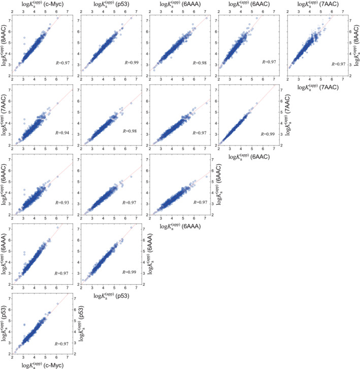
Correlations of the ligand‐binding profiles between any two IDPs. Each data point represents the binding affinities (measured by ) of a ligand with two IDPs. The solid line represents a linear fit with the Pearson's coefficient displayed in each panel. For the sake of clarity, error bars estimated from bootstrap method were only plotted in the top‐right panel, and some details were provided in Figure S1. IDP, intrinsically disordered protein
The intriguing correlation also holds for the IDPs‐binding profiles between different ligands, with the example of a few ligands shown in Figure 3. Different ligands have different affinities to IDPs, for example, the affinity of the strongest binder (Lig740) lies within 5.5–7.5, being much higher than that of 10074‐A4 of 3.5–5.0, but the linear correlation is significant between them. The statistics of correlation coefficient for all ligand pairs is given in Figure S3, resulting in an average value of 0.97.
FIGURE 3.

Correlations of the IDPs‐binding profiles of 10074‐A4 and a few other ligands. Lig740 is the ligand with the highest affinity among all 560 ligands. The data points represents the binding affinities () to different IDPs: (from left to right) 6AAC, 7AAC, c‐Myc, p53, 6AAA, and 8AAC. IDP, intrinsically disordered protein
2.2. Decomposition of binding affinity
The ligand capacity is the general potential of a ligand to bind various proteins (IDPs), so we quantitatively calculate ligand capacity of the ligand‐ by
| (2) |
where is the number of IDPs in our study. Similarly, the ligandability as the general potential of an IDP to bind various ligands is calculated by
| (3) |
where is the number of ligands. The determined for 6 IDPs (c‐Myc, p53, 6AAA, 6AAC, 7AAC, and 8AAC) are , , , , and , respectively, where the error bars were estimated based on the bootstrap method. The distribution of for 560 ligands lies between 2.0 and 6.0 and can be approximately described by a Gaussian distribution (Figure S4) with an average of 3.9.
The revealed linear relationships between the binding profiles between different proteins or ligands above (Figures 2 and 3) suggest that the binding affinities between IDPs and ligands ( matrix) are more regular than expected, and the number of required parameters may be much smaller than . We have analysed the representation of affinity matrix (see the Supporting Information for more details) and find that the binding affinity can be approximately expressed by the ligandability of IDPs and the ligand capacity of ligands as
| (4) |
where is a constant to account for the double‐counting contribution from protein and ligand, which is equal to the average value of , that is, . The numerical result is depicted in Figure 4, where the approximation seems excellent. The reconstructed with Equation (4) reproduce the original ones accurately, with a correlation coefficient of . The average discrepancy is as small as 0.11. An extra ‐test indicates that the ratio between the calculated value and the number of degrees of freedom is 0.63, confirming the quality of linear decomposition.
FIGURE 4.
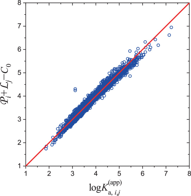
Effect of expressing the binding affinities () in terms of the ligandability of IDPs and the ligand capacity of ligands. IDP, intrinsically disordered protein
The decomposition of the binding affinity leads to a remarkable prediction that, given a particular set of ligand molecules, the ordering of their binding affinities is highly similar for any IDP. This can be demonstrated in Figure 5, where the ligand‐binding profiles of each IDP were plotted as a function of the ranking order of the ligand capacity which is now calculated from the other IDPs. Approximately, decreases monotonically with the ranking order of for any IDP. When was estimated from only one IDP, the monotonic descent tendency still exists (Figure S5).
FIGURE 5.

Ligand‐binding affinity profiles for each IDP as a function of the ranking order of the ligand capacity calculated without the specified each IDP: (a) c‐Myc, (b) p53, (c) 6AAA, (d) 6AAC, (e) 7AAC, and (f) 8AAC. The data of the ‐axis are excluded from the calculation of of the ‐axis in each panel. IDP, intrinsically disordered protein
The novel property of IDPs revealed here has significant potential applications. It suggests that the data obtained in some IDPs may have a great generalization ability to predict the property of a new IDP. For example, the aim of virtual screening upon IDP‐ is to pick out top ligands with larger than those of others ligands . Despite the efficiency of single docking calculation, the huge number of conformations in the ensemble still makes the virtual screening upon IDPs time‐consuming. Even if reinforcement learning can be used to greatly accelerate the process, 43 virtual screening upon IDPs keeps slower than that for ordered proteins. However, with Equation (4), it is noted that the ordering of with fixed depends merely on and is independent on . This means that if we summarize from the results of some known IDPs, the virtual screening result on a new IDP‐ can be directly interpreted/extrapolated from previous experiences without the IDP‐ docking calculation. We test this idea by using the docking data for five IDPs (each with 100 conformations) other than c‐Myc to calculate and predict the affinity ordering of 560 ligands against c‐Myc. The prediction performance is assessed by comparing with the “real” results based on direct docking of c‐Myc (with 16,716 conformations). The adopted metrics to measure the performance is the enrichment factor (), defined as the concentration of the real top ligands (under the specified positive rate ) among the predicted top ligands (under the predicted positive rate ) compared to their concentration throughout the entire ligand dataset, that is, 44
| (5) |
where is the ranking number in a descending order. Alternatively, can be calculated as where , , , and represent the sample number of true positive, false positive, true negative, and false negative, respectively. The analyses were presented in Figure 6 for a positive rate () of about 1% and 10%, respectively. Even without using the docking data of c‐Myc, the prediction achieves a very high enrichment factor approaching the upper limit (red solid lines in Figure 6). At a positive rate of 1% (aiming at predicting the top five ligands), the prediction successfully picks 4 out 5 top ligands at the same predicted positive rate, giving a precision of 80%, which is even slightly higher than that in reinforcement learning (78%). 43 The strong correlation of the binding affinities of a ligand with different IDPs hints that IDPs may become a promising field of “new uses for old drugs.” 45 As a supporting example, 10074‐G5, a previous known ligand to inhibit c‐Myc‐Max heterodimerization, was recently confirmed by experiments to binds monomeric Aβ42, a disordered peptide unrelated to c‐Myc. 46
FIGURE 6.

Enrichment factor of using to predict the binding affinity to c‐Myc. here is determined from the data for p53, 6AAA, 6AAC, 7AAC, and 8AAC. The positive rate is set to be (a) ~1% (with 5 among 560 ligands with top affinity set to be positive samples, and strictly speaking, ) and (b) 10% (with 56 top ligands to be positive). The red solid lines represent the upper limit of enrichment factor when the prediction is exactly identical to the “real” value. The vertical dashed lines indicate the positive rate value
2.3. Origin of the universal linear correlation
We now turn to the possible origin of the revealed simple behavior of IDPs. One may suspect that the ligand capacity is merely caused by some simple molecular properties. For example, molecular weight is one of the main factors influencing the binding affinity, as the maximal affinity per atom is about −1.5 kcal/mol for organic ligands. 47 , 48 However, the analysis in Figure S6 shows that although the binding affinity roughly increases with the molecular weight of ligand, the correlation is too low to explain the strong linear relationships observed previously in Figure 2. The key to understanding the observed simplicity likely lies in the averaging process over conformations. The idea is roughly demonstrated in Figure 7 using c‐Myc and 10074‐A4 as the IDP‐ligand pair. When we examine the conformation‐specified binding affinity instead of the ensemble‐averaged result as given by Equation (1), it is uncorrelated with the CavityScore (a quantity given by the cavity test program CAVITY 42 to describe the potential affinity with ligand) as shown in Figure 7a. However, if we bin the conformations with similar CavityScore together and calculate their average binding affinity, a simple linear relationship appears between the binning average of affinity and the CavityScore (especially for those with a large number of conformations) (Figure 7b). 2 Recalling that the apparent binding affinity is an average over all the conformational ensemble, it is not unreasonable for IDPs to possess properties reflecting some kind of inherent nature with greatly suppressed fluctuations. From this point of view, more is simpler.
FIGURE 7.

(a) Correlation between the CavityScore of 16,716 conformations of c‐Myc and their individual binding affinity to the ligand 10074‐A4 where with indicates conformations in the ensemble of IDP‐ as that in Equation (1). (b) The binning average of (a) with a bin‐width of 100 for CavityScore, that is, the original data points in (a) were divided into small intervals (bins) of CavityScore and the average of of data points in each bins was calculated to be shown in (b). IDP, intrinsically disordered protein
The observed universal linear correlations may arise from both physicochemical and mathematical reasons. From a chemical point of view, different proteins (ligands) have different general potential (propensity) in binding various targets, resulting in metrics such as and . From a mathematical point of view, and pose a constraint on the probability of the binding affinity between protein‐ and ligand‐, which can be inferred with Bayesian probability theory 49 to give (see Supporting Information):
| (6) |
where is a random variable with a zero mean. Whether the linear correlation is good or poor depends on the variance of the fluctuating . An IDP exists in an ensemble of highly heterogeneous conformations, and each conformation‐ can be approximately regarded as an ordered protein. The apparent affinity of an IDP is some kind of average over its conformational ensemble. Mathematically, the fluctuation variance of the average is always smaller than that of a single sample. Consequently, the linear relation for IDPs is much better than that for ordered proteins (see Supporting Information for more details).
2.4. Ordered proteins
Finally, the concepts and insights obtained above for IDPs are applied to conventional ordered proteins to demonstrate their difference with IDPs (Figure 8). The dataset of ordered proteins was adopted from CavityTEST, 50 which contains 35 structurally distinct proteins. Molecular docking with AutoDock Vina was used to estimate their binding free energies with ligands. To some extent, the binding affinity of ligands to one protein is correlated to that to another protein (some examples shown in Figure 8a), but the correlation coefficient (with an average of 0.82) is much smaller than that for IDPs (0.97). Similar phenomena were observed for ordered proteins with NMR structures (Figures S7 and S8), suggesting that the influence of conformation ensemble for ordered proteins is negligible. For the protein‐binding profiles between different ligands, the correlation is even weaker (some shown in Figure 8b), with an average correlation coefficient of only 0.6. The origin is that order proteins have unique conformations and the binding affinity with a ligand depends more on their specific interactions. To achieve an effect similar to conformational averaging, we calculate the ligand capacity to ordered proteins as the average binding affinity as that in Equation (2). By averaging over different proteins, the obtained reflects the general potential of a ligand to bind various ordered proteins, which is nicely correlated to the IDPs case (Figure 8c). has limited power in predicting the virtual screening result for ordered proteins (Figure 8d). At a positive rate of 1%, the average precision of prediction is 47%. We also test the decomposition of binding affinity for ordered proteins into a sum of and as Equation (4), and the resulting average discrepancy is 0.38 (see Figure S9), almost four times as large as that for IDPs.
FIGURE 8.

Corresponding properties in ordered proteins. (a) Correlations of the ligand‐binding profiles for some ordered proteins with given PDB IDs. (b) Correlations of the protein binding profiles for some ligands. (c) Correlation between the ligand capacity to bind IDPs and that to bind ordered proteins. The solid lines in (a–c) represent linear fits. (d) The enrichment factor of using to predict the virtual screening (ordering of binding affinity) to ordered proteins. A leave‐one‐out scheme was adopted, that is, one protein is chosen as the predicted system with calculated from the others proteins. The black solid line represents the upper limit of enrichment factor and the vertical dashed line indicates the positive rate value. IDP, intrinsically disordered protein
We have also compared the ligand binding profiles between ordered and disordered proteins (some examples in Figure 9, and more examples in Figure S10). There are linear correlations between them, and the average correlation coefficient (0.89) lies between that for order proteins (0.82) and that for IDPs (0.97).
FIGURE 9.

Correlations of the ligand‐binding profiles between ordered proteins (with PDB IDs 4CA2 and 1A4J) and IDPs (c‐Myc and p53). IDP, intrinsically disordered protein
3. DISCUSSION
The results in this study are helpful for understanding the specificity of protein–ligand binding. To possess a high specificity, a ligand is expected to bind the target protein with an affinity significantly higher than its binding to other non‐targets. The observed (over)simplified behaviors of binding affinity represent a baseline of protein–ligand binding. The strong correlation between binding profiles for different IDPs and the decomposability of ligand‐IDPs affinity suggest that a ligand has a strong tendency to bind non‐target IDPs if it binds strongly to the targeted IDPs. This is obviously unfavorable for achieving specificity. To achieve a high specificity, the binding profile needs to deviate from the average/baseline behavior of Equation (4), for example, to further increase the affinity to target and decreases those to non‐targets. The fluctuating discrepancy for ordered proteins is much larger than that for IDPs, so it is more difficult to control the specificity of IDPs.
It is worth noting that the binding free energy was estimated in this study by molecular docking based on empirical scoring functions, which were usually less sensitive (more robust) to the variation of detailed conformations. When using more physicochemical approaches such as molecular simulations employing all‐atom force fields, would be more sensitive to the molecular details of conformation, leading to a magnified specificity. This may be why in reality, even for IDPs, specificity is possible (though difficult).
It is also noted that ligands of experimental interests often exhibit a strong target‐binding behavior. If we focus on such a high regime, there would be less correlation than the whole binding spectrum such as that in Figure 2. Furthermore, the protein–ligand‐binding cases considered in this study may not be exactly the same as the biological effect, that is, more concerned in practical therapies. It is highly probable that the conformational ensemble would be restrained in some specific states of biological relevance due to the binding of external agents. However, this conformational drift is actually not modelled in the current work, which could be a limitation that should be addressed in future work.
4. CONCLUSION
In summary, we have analyzed the binding affinities of a spectrum of ligands with many IDPs and observed a robust linear correlation among the binding profiles for different IDPs as well as for different ligands. The average correlation coefficient is as high as 0.97. As a result, the affinity can be approximately expressed as a sum of the ligandability of IDPs and the ligand capacity . Such an unexpected regularity can be utilized to perform virtual screening upon IDPs, where a precision of 80% was achieved in an illustrative calculation on c‐Myc at a positive rate of 1% even without direct docking on it. On the other hand, the regularity gives rise to the lower specificity of IDPs‐ligand‐binding compared with conventional ordered proteins and thus constitutes an obstacle for drug design upon IDPs.
AUTHOR CONTRIBUTIONS
Xiaohui Wang: Data curation (equal); investigation (equal); methodology (equal); validation (equal); writing – original draft (equal). Bin Chong: Data curation (equal); formal analysis (equal); investigation (equal); methodology (equal); writing – original draft (equal). Zhaoxi Sun: Data curation (equal); formal analysis (equal); investigation (equal); software (equal); validation (equal); writing – original draft (equal). Hao Ruan: Data curation (equal). Yingguang Yang: Software (equal). Pengbo Song: Software (equal). Zhirong Liu: Conceptualization (equal); formal analysis (equal); funding acquisition (equal); investigation (equal); methodology (equal); project administration (equal); supervision (equal); visualization (equal); writing – original draft (equal); writing – review and editing (equal).
Supporting information
Figure S1. Correlation of the ligand binding profiles between IDPs 7AAC and 8AAC with error bars estimated from bootstrap method. (a, c) The binding in an ascending index for 7AAC and 8AAC, respectively. (b) The correlation of binding profiles between 7AAC and 8AAC.
Figure S2. 3D plot of the correlations of the ligand binding profiles for c‐Myc, p53 and 8AAC. Each blue raw data point represents the binding affinities of a ligand with three IDPs (c‐Myc, p53 and 8AAC). The red thick line represents a 3D linear fit.
Figure S3. Distribution of the correlation coefficient for the IDPs‐binding profiles between different ligands. The average value is 0.97. The number of ligand pairs is 560 × 559/2 = 156,520.
Figure S4. Distribution of the ligand capacity of 560 ligands, with solid curves as the fitted Gaussian function. The mean value is 3.9.
Figure S5. Correlation between the ligand‐binding affinity profiles of IDPs and the ranking order of the binding affinity to c‐Myc. The ligand‐binding affinity profiles for each IDP was plotted as a function of the ranking order of for c‐Myc (i.e., the ranking order of calculated from only c‐Myc).
Figure S6. Correlation between the molecular weight of 560 ligands and their binding affinity to c‐Myc.
Figure S7. Distribution of the ligand binding affinity for six ordered proteins with NMR structure. Solid curves represent the fitted Gaussian function. It is noted that the fitting for 1DF3 and 5LNF is poor because there are some abnormal data in the low region, probably due to the small cavity they possess.
Figure S8. Correlations of the ligand binding profiles for some ordered proteins with NMR structure. The solid line represents a linear fit with the Pearson's coefficient 𝑅 displayed in each panel. The average 𝑅 value is 0.80. 1DF3 and 5LNF were not included because their distributions in Figure S7 are abnormal.
Figure S9. The effect of expressing the binding affinities in terms of the ligandability of ordered proteins and the ligand capacity of ligands. 𝐶0 = 4.8, higher than the value (3.9) in IDPs, so IDPs have relatively lower affinity.
Figure S10. Correlations of the ligand binding profiles between ordered proteins (𝑦‐axis, with given PDB IDs) and IDPs (𝑥‐axis). The solid line represents a linear fit with the Pearson's coefficient 𝑅 displayed in each panel.
Figure S11. The distribution of binding affinities between ordered proteins and ligands, with the solid curve as the fitted Gaussian function.
ACKNOWLEDGMENTS
This work was supported by the Beijing Natural Science Foundation (grant 7224357) and the National Natural Science Foundation of China (grant 21633001). Part of the analysis was performed on the High‐Performance Computing Platform of the Center for Life Science (Peking University). We thank Prof. Luhua Lai, Prof. Yongqi Huang, Dr. Qiaojing Huang, and Dr. Limin Chen for helpful discussions.
Wang X, Chong B, Sun Z, Ruan H, Yang Y, Song P, et al. More is simpler: Decomposition of ligand‐binding affinity for proteins being disordered. Protein Science. 2022;31(7):e4375. 10.1002/pro.4375
Xiaohui Wang and Bin Chong contributed equally to this work.
Review Editor: Nir Ben‐Tal
Funding information National Natural Science Foundation of China, Grant/Award Number: 21633001; Beijing Natural Science Foundation, Grant/Award Number: 7224357
ENDNOTES
From a theoretical perspective, there exist interactions (hydrophobic interaction, electrostatic interaction, and van der Waals interaction) between any protein and ligand, whether strong or weak, leading to a certain affinity. On the other hand, in experiments only those with an affinity above some certain thresholds were detectable or measurable. In other words, from an experimental perspective, there is no interaction between many proteins and ligands (and thus is meaningless to discuss the affinity in these cases). In this theoretical study, the protein–ligand interaction and affinity were discussed in the former sense.
In the high CavityScore region, the binning‐average results deviate from the linear relationship. It is unclear whether such a deviation was caused by the few original data points available therein or some unknown intrinsic property.
REFERENCES
- 1. Meyer B, Peters T. NMR spectroscopy techniques for screening and identifying ligand binding to protein receptors. Angew Chem Int Ed. 2003;42:864–890. [DOI] [PubMed] [Google Scholar]
- 2. Jorgensen WL. The many roles of computation in drug discovery. Science. 2004;303:1813–1818. [DOI] [PubMed] [Google Scholar]
- 3. Wang L, Wu YJ, Deng YQ, et al. Accurate and reliable prediction of relative ligand binding potency in prospective drug discovery by way of a modern free‐energy calculation protocol and force field. J Am Chem Soc. 2015;137:2695–2703. [DOI] [PubMed] [Google Scholar]
- 4. Huang YQ, Liu ZR. Do intrinsically disordered proteins possess high specificity in protein–protein interactions? Chem Eur J. 2013;19:4462–4467. [DOI] [PubMed] [Google Scholar]
- 5. Volkamer A, Kuhn D, Grombacher T, Rippmann F, Rarey M. Combining global and local measures for structure‐based druggability predictions. J Chem Inf Model. 2012;52:360–372. [DOI] [PubMed] [Google Scholar]
- 6. Halgren TA. Identifying and characterizing binding sites and assessing druggability. J Chem Inf Model. 2009;49:377–389. [DOI] [PubMed] [Google Scholar]
- 7. Hussein HA, Geneix C, Petitjean M, Borrel A, Flatters D, Camproux AC. Global vision of druggability issues: Applications and perspectives. Drug Discov Today. 2017;22:404–415. [DOI] [PubMed] [Google Scholar]
- 8. Lipinski CA, Lombardo F, Dominy BW, Feeney PJ. Experimental and computational approaches to estimate solubility and permeability in drug discovery and development settings. Adv Drug Deliv Rev. 1997;23:3–25. [DOI] [PubMed] [Google Scholar]
- 9. Leeson PD, Davis AM. Time‐related differences in the physical property profiles of oral drugs. J Med Chem. 2004;47:6338–6348. [DOI] [PubMed] [Google Scholar]
- 10. Hann MM, Oprea TI. Pursuing the leadlikeness concept in pharmaceutical research. Curr Opin Chem Biol. 2004;8:255–263. [DOI] [PubMed] [Google Scholar]
- 11. Kenakin T, Onaran O. The ligand paradox between affinity and efficacy: Can you be there and not make a difference? Trends Pharmacol Sci. 2002;23:275–280. [DOI] [PubMed] [Google Scholar]
- 12. Bickerton GR, Paolini GV, Besnard J, Muresan S, Hopkins AL. Quantifying the chemical beauty of drugs. Nat Chem. 2012;4:90–98. [DOI] [PMC free article] [PubMed] [Google Scholar]
- 13. Wright PE, Dyson HJ. Intrinsically unstructured proteins: Re‐assessing the protein structure‐function paradigm. J Mol Biol. 1999;293:321–331. [DOI] [PubMed] [Google Scholar]
- 14. Uversky VN, Gillespie JR, Fink AL. Why are “natively unfolded” proteins unstructured under physiologic conditions? Proteins. 2000;41:415–427. [DOI] [PubMed] [Google Scholar]
- 15. Liu ZR, Huang YQ. Advantages of proteins being disordered. Protein Sci. 2014;23:539–550. [DOI] [PMC free article] [PubMed] [Google Scholar]
- 16. van der Lee R, Buljan M, Lang B, et al. Classification of intrinsically disordered regions and proteins. Chem Rev. 2014;114:6589–6631. [DOI] [PMC free article] [PubMed] [Google Scholar]
- 17. Uversky VN, Oldfield CJ, Dunker AK. Intrinsically disordered proteins in human diseases: Introducing the D2 concept. Annu Rev Biophys. 2008;37:215–246. [DOI] [PubMed] [Google Scholar]
- 18. Metallo SJ. Intrinsically disordered proteins are potential drug targets. Curr Opin Chem Biol. 2010;14:481–488. [DOI] [PMC free article] [PubMed] [Google Scholar]
- 19. Tsafou K, Tiwari PB, Forman‐Kay JD, Metallo SJ, Toretsky JA. Targeting intrinsically disordered transcription factors: Changing the paradigm. J Mol Biol. 2018;430:2321–2341. [DOI] [PubMed] [Google Scholar]
- 20. Chong B, Li MD, Li T, Yu M, Zhang YG, Liu ZR. Conservation of potentially druggable cavities in intrinsically disordered proteins. ACS Omega. 2018;3:15643–15652. [DOI] [PMC free article] [PubMed] [Google Scholar]
- 21. Biesaga M, Frigole‐Vivas M, Salvatella X. Intrinsically disordered proteins and biomolecular condensates as drug targets. Curr Opin Chem Biol. 2021;62:92–100. [DOI] [PMC free article] [PubMed] [Google Scholar]
- 22. Yin XY, Giap C, Lazo JS, Prochownik EV. Low molecular weight inhibitors of Myc‐max interaction and function. Oncogene. 2003;22:6151–6159. [DOI] [PubMed] [Google Scholar]
- 23. Yu C, Niu X, Jin F, Liu Z, Jin C, Lai L. Structure‐based inhibitor design for the intrinsically disordered protein c‐Myc. Sci Rep. 2016;6:22298. [DOI] [PMC free article] [PubMed] [Google Scholar]
- 24. Toth G, Gardai SJ, Zago W, et al. Targeting the intrinsically disordered structural ensemble of alpha‐Synuclein by small molecules as a potential therapeutic strategy for Parkinson's disease. PLoS One. 2014;9:87133. [DOI] [PMC free article] [PubMed] [Google Scholar]
- 25. Krishnan N, Koveal D, Miller DH, et al. Targeting the disordered C terminus of PTP1B with an allosteric inhibitor. Nat Chem Biol. 2014;10:558–566. [DOI] [PMC free article] [PubMed] [Google Scholar]
- 26. De Mol E, Fenwick RB, Phang CTW, et al. EPI‐001, a compound active against castration‐resistant prostate cancer, targets transactivation unit 5 of the androgen receptor. ACS Chem Biol. 2016;11:2499–2505. [DOI] [PMC free article] [PubMed] [Google Scholar]
- 27. Ruan H, Yu C, Niu XG, et al. Computational strategy for intrinsically disordered protein ligand design leads to the discovery of p53 transactivation domain I binding compounds that activate the p53 pathway. Chem Sci. 2021;12:3004–3016. [DOI] [PMC free article] [PubMed] [Google Scholar]
- 28. Silvestre‐Roig C, Braster Q, Wichapong K, et al. Externalized histone H4 orchestrates chronic inflammation by inducing lytic cell death. Nature. 2019;569:236–240. [DOI] [PMC free article] [PubMed] [Google Scholar]
- 29. Chen LM, Cheng BM, Sun Q, Lai LH. Ligand‐based optimization and biological evaluation of N‐(2,2,2‐trichloro‐1‐[3‐phenylthioureido]ethyl)acetamide derivatives as potent intrinsically disordered protein c‐Myc inhibitors. Bioorg Med Chem Lett. 2021;31:127711. [DOI] [PubMed] [Google Scholar]
- 30. Jin F, Yu C, Lai LH, Liu ZR. Ligand clouds around protein clouds: A scenario of ligand binding with intrinsically disordered proteins. PLoS Comput Biol. 2013;9:e1003249. [DOI] [PMC free article] [PubMed] [Google Scholar]
- 31. Su XY, Wang K, Liu N, Chen JW, Li Y, Duan MJ. All‐atom structure ensembles of islet amyloid polypeptides determined by enhanced sampling and experiment data restraints. Proteins. 2019;87:541–550. [DOI] [PubMed] [Google Scholar]
- 32. Knott M, Best RB. Discriminating binding mechanisms of an intrinsically disordered protein via a multi‐state coarse‐grained model. J Chem Phys. 2014;140:175102. [DOI] [PMC free article] [PubMed] [Google Scholar]
- 33. Fuxreiter M. Fuzziness: Linking regulation to protein dynamics. Mol Biosyst. 2012;8:168–177. [DOI] [PubMed] [Google Scholar]
- 34. Swendsen RH. An introduction to statistical mechanics and thermodynamics. New York: Oxford University Press; 2012. [Google Scholar]
- 35. Chong B, Yang YG, Zhou CG, Huang QJ, Liu ZR. Ensemble‐based thermodynamics of the fuzzy binding between intrinsically disordered proteins and small‐molecule ligands. J Chem Inf Model. 2020;60:4967–4974. [DOI] [PubMed] [Google Scholar]
- 36. Wang X, Sun Z. A theoretical interpretation of variance‐based convergence criteria in perturbation‐based theories. arXiv. 2018;1803.03123. [Google Scholar]
- 37. Wang RX, Lai LH, Wang SM. Further development and validation of empirical scoring functions for structure‐based binding affinity prediction. J Comput Aided Mol Des. 2002;16:11–26. [DOI] [PubMed] [Google Scholar]
- 38. Morris GM, Goodsell DS, Halliday RS, et al. Automated docking using a Lamarckian genetic algorithm and an empirical binding free energy function. J Comput Chem. 1998;19:1639–1662. [Google Scholar]
- 39. Trott O, Olson AJ. AutoDock Vina: Improving the speed and accuracy of docking with a new scoring function, efficient optimization, and multithreading. J Comput Chem. 2010;31:455–461. [DOI] [PMC free article] [PubMed] [Google Scholar]
- 40. Varadi M, Kosol S, Lebrun P, et al. pE‐DB: A database of structural ensembles of intrinsically disordered and of unfolded proteins. Nucleic Acids Res. 2014;42:D326–D335. [DOI] [PMC free article] [PubMed] [Google Scholar]
- 41. Lazar T, Martinez‐Perez E, Quaglia F, et al. PED in 2021: A major update of the protein ensemble database for intrinsically disordered proteins. Nucleic Acids Res. 2021;49:D404–D411. [DOI] [PMC free article] [PubMed] [Google Scholar]
- 42. Yuan YX, Pei JF, Lai LH. Binding site detection and druggability prediction of protein targets for structure‐based drug design. Curr Pharm Design. 2013;19:2326–2333. [DOI] [PubMed] [Google Scholar]
- 43. Chong B, Yang YG, Wang ZL, Xing H, Liu ZR. Reinforcement learning to boost molecular docking upon protein conformational ensemble. Phys Chem Chem Phys. 2021;23:6800–6806. [DOI] [PubMed] [Google Scholar]
- 44. Truchon JF, Bayly CI. Evaluating virtual screening methods: Good and bad metrics for the “early recognition” problem. J Chem Inf Model. 2007;47:488–508. [DOI] [PubMed] [Google Scholar]
- 45. Chong CR, Sullivan DJ. New uses for old drugs. Nature. 2007;448:645–646. [DOI] [PubMed] [Google Scholar]
- 46. Heller GT, Aprile FA, Michaels TCT, et al. Small‐molecule sequestration of amyloid‐beta as a drug discovery strategy for Alzheimer's disease. Sci Adv. 2020;6:eabb5924. [DOI] [PMC free article] [PubMed] [Google Scholar]
- 47. Kuntz ID, Chen K, Sharp KA, Kollman PA. The maximal affinity of ligands. Proc Natl Acad Sci U S A. 1999;96:9997–10002. [DOI] [PMC free article] [PubMed] [Google Scholar]
- 48. Hopkins AL, Groom CR, Alex A. Ligand efficiency: A useful metric for lead selection. Drug Discov Today. 2004;9:430–431. [DOI] [PubMed] [Google Scholar]
- 49. Jaynes ET. Probability theory: The logic of science. Cambridge University Press, Cambridge; 2003. [Google Scholar]
- 50. Laurie ATR, Jackson RM. Q‐SiteFinder: An energy‐based method for the prediction of protein‐ligand binding sites. Bioinformatics. 2005;21:1908–1916. [DOI] [PubMed] [Google Scholar]
Associated Data
This section collects any data citations, data availability statements, or supplementary materials included in this article.
Supplementary Materials
Figure S1. Correlation of the ligand binding profiles between IDPs 7AAC and 8AAC with error bars estimated from bootstrap method. (a, c) The binding in an ascending index for 7AAC and 8AAC, respectively. (b) The correlation of binding profiles between 7AAC and 8AAC.
Figure S2. 3D plot of the correlations of the ligand binding profiles for c‐Myc, p53 and 8AAC. Each blue raw data point represents the binding affinities of a ligand with three IDPs (c‐Myc, p53 and 8AAC). The red thick line represents a 3D linear fit.
Figure S3. Distribution of the correlation coefficient for the IDPs‐binding profiles between different ligands. The average value is 0.97. The number of ligand pairs is 560 × 559/2 = 156,520.
Figure S4. Distribution of the ligand capacity of 560 ligands, with solid curves as the fitted Gaussian function. The mean value is 3.9.
Figure S5. Correlation between the ligand‐binding affinity profiles of IDPs and the ranking order of the binding affinity to c‐Myc. The ligand‐binding affinity profiles for each IDP was plotted as a function of the ranking order of for c‐Myc (i.e., the ranking order of calculated from only c‐Myc).
Figure S6. Correlation between the molecular weight of 560 ligands and their binding affinity to c‐Myc.
Figure S7. Distribution of the ligand binding affinity for six ordered proteins with NMR structure. Solid curves represent the fitted Gaussian function. It is noted that the fitting for 1DF3 and 5LNF is poor because there are some abnormal data in the low region, probably due to the small cavity they possess.
Figure S8. Correlations of the ligand binding profiles for some ordered proteins with NMR structure. The solid line represents a linear fit with the Pearson's coefficient 𝑅 displayed in each panel. The average 𝑅 value is 0.80. 1DF3 and 5LNF were not included because their distributions in Figure S7 are abnormal.
Figure S9. The effect of expressing the binding affinities in terms of the ligandability of ordered proteins and the ligand capacity of ligands. 𝐶0 = 4.8, higher than the value (3.9) in IDPs, so IDPs have relatively lower affinity.
Figure S10. Correlations of the ligand binding profiles between ordered proteins (𝑦‐axis, with given PDB IDs) and IDPs (𝑥‐axis). The solid line represents a linear fit with the Pearson's coefficient 𝑅 displayed in each panel.
Figure S11. The distribution of binding affinities between ordered proteins and ligands, with the solid curve as the fitted Gaussian function.