Modified Flowing Material Balance Equation for Shale Gas Reservoirs

Abstract

To determine original gas-in-place, this study establishes a flowing material balance equation based on the improved material balance equation for shale gas reservoirs. The method considers the free gas in the matrix and fracture, the dissolved gas in kerogen, and the pore volume occupied by adsorbed phase simultaneously, overcoming the problem of incomplete consideration in the earlier models. It also integrates the material balance method with the flowing material balance method to obtain the average formation pressure, eliminating the problem with the previous method where shutting down of wells was needed to monitor the formation pressure. The volume of the adsorbed gas on the ground is converted into volume of the adsorbed phase in the formation using the volume conservation method to characterize the pore volume occupied by the adsorbed phase, which solves the problem of the previous model that the adsorbed phase was neglected in the pore volume. The model proposed in this study is applied to the Fuling Shale Gas Field in southwest China and compared with other flowing material balance equations, and the results show that the single-well control area calculated by the model proposed in this study is closer to the real value, indicating that the calculations in this study are more accurate. Furthermore, the calculations show that the dissolved gas takes up a large fraction of the total reserves and cannot be ignored. The sensitivity analyses of critical parameters demonstrate that (a) the greater the porosity of the fracture, the greater the free gas storage; (b) the values of Langmuir volume and TOC can significantly affect the results of the reservoir calculation; and (c) the adsorbed phase occupies a smaller pore volume when the Langmuir volume is smaller, the Langmuir pressure is higher, or the adsorbed phase density is higher. The findings of this study can provide better understanding of the necessity to take into account the dissolved gas in the kerogen, the pore volume occupied by the adsorbed phase, and the fracture porosity when evaluating reserves. The method could be applied to the calculation of pressure, recovery of free gas phase and adsorbed phase, original gas-in-place, and production predictions, which could help for better guidance of reserve potential estimations and development strategies of shale gas reservoirs.

1. Introduction

With the increase of the world energy demand, unconventional gas resources have attracted attention worldwide.¹⁻³ Compared to conventional gas reservoirs, shale gas has its characteristics. First, shale has extremely low permeability and high heterogeneity. Re-equilibrium of the fluids will be time-consuming for the build-up well tests, and a material balance equation based on the static and dynamic reservoir parameters could be an expected method to characterize the shale gas reservoirs. Second, in terms of storage mechanism, gas mainly exists in adsorbed, free, and dissolved states in the shale.⁴⁻⁷ Thus, the calculation methods for conventional reserves may not be applied to shale gas.^8,9 Previous scholars studied the calculation of the original gas-in-place (OGIP) of shale gas, and factors such as free gas, adsorbed gas, dissolved gas, rock stress sensitivity, and irreducible water expansion have been taken into consideration, making their models closer to the real gas reservoir.¹⁰⁻¹³ However, there are still important factors that have not been considered, including the influence of free gas in the fracture and the volume of the adsorbed phase in the pore space. The above factors should be considered comprehensively to calculate the OGIP of shale gas accurately.

The material balance equation of coalbed methane considering the effects of water influx and adsorbed gas was first proposed by King.¹⁰ The OGIP could be calculated using the slope and intercept of p/Z* (ratio of pressure and modified Z-factor) versus G_p (cumulative gas production). Based on King’s work, Ahmed et al.¹¹ established the material balance equation of coalbed methane considering free gas, adsorbed gas, irreducible water expansion, and stress sensitivity, and they applied it to solve the average formation pressure. Moghadam et al.¹⁴ redefined the Z-factor according to the principle of volume conservation and extended the material balance equation to all gas reservoirs and used the bottom hole pressure (BHP) to calculate OGIP when in a pseudo-steady flow. Mattar and McNeil¹⁵ proposed the flowing material balance method, which used BHP instead of average formation pressure to calculate reserves. Anderson et al.¹⁶ proposed material balance pseudo-time and extended this method from constant BHP or constant production rate to changed production rates and changed production pressures. Considering the adsorbed gas, the flowing material balance equation of the coalbed methane reservoir was established by Clarkson et al.¹⁷

However, according to Ambrose et al.,¹⁸ the volume of adsorbed phase could not be ignored, and the volume of the adsorbed phase needs to be subtracted from the void space measured by porosity measurement (Figure 1). The previously mentioned material balance equations did not consider the pore volume occupied by the adsorbed phase and overestimated the volume occupied by the free gas, resulting in inaccurate calculations of total reserves. In addition, shale gas has the characteristics of low permeability and high heterogeneity, necessitating hydraulic fracturing to achieve industrial production.¹⁹⁻²¹ The compressibility of fracture is much higher than that of the matrix, and the porosity of fracture and matrix varies with pressure.²²⁻²⁵ Thus, the influence of fracture should be considered in the improved material balance equations. As free gas is produced and formation pressure drops, the adsorbed gas begins to desorb and dissolved gas begins to diffuse, supplying formation energy. Thus, the mechanism of adsorbed gas desorption and dissolved gas diffusion should be considered in the new method.

Figure 1.

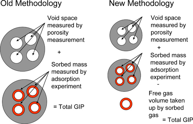
Comparison of the old and new methodologies in predicting shale gas-in-place. Reprinted (adapted or reprinted in part) with permission from ref 18.

The influences of adsorbed phase volume, dissolved gas, and free gas on fracture were not fully included in prior approaches for computing reserves of shale gas reservoirs, resulting in discrepancies in reserve calculation results.²⁶⁻³⁰ The adsorption model and multiscale gas fluid flow are considered to describe the volume change of gas adsorption/desorption and gas dissolution. By rebuilding the pore volume model, the volume change of gas in kerogen, matrix, and fractures, the volume changes due to stress sensitivity and irreducible water expansion, and volume change due to adsorbed gas desorption are considered. Thus, based on the previous studies, this study integrates various factors (adsorbed phase occupying pore volume, dissolved gas in kerogen, free gas in both fracture and matrix, stress sensitivity, irreducible water expansion, and adsorbed gas) to establish a new material balance equation for shale gas reservoirs, addressing issues such as the inadequacy of prior methods to account for free gas in fractures, pore volume occupied by adsorbed gas, and the challenging problem of obtaining formation pressure. The general sketch diagram of the method used in this study is shown in Figure 2.

Figure 2.

General sketch diagram of the study problem.

In this study, the shale gas reservoir material balance method considering multiple factors and the flowing material balance method is established in Section 2. The accuracy of the method proposed in this study is verified in Section 3.1. The gas rate is predicted in Section 3.2 using the method proposed in this study. The sensitivity analysis of critical parameters is detailed in Section 3.3. The advantages, disadvantages, and limitations of the proposed method are given in Section 3.4. The summary and conclusions of this study are given in Section 4.

2. Methodology

This study has the following assumptions when the material balance equations are established for shale gas reservoirs: (1) shale gas reservoirs are isothermal; (2) matrix and fractures systems have different irreducible water saturation; (3) water influx and water production are not considered and only free gas flows in the fracture are considered;³¹ (4) adsorbed gas is adsorbed on the inner surface of the matrix; and (5) shale gas reservoirs have double porosity (matrix, fractures) and single permeability (fractures).

The shale gas mainly contains adsorbed, free, and dissolved gas stored in the matrix and fractures. The OGIP contains four parts: the adsorbed gas in the matrix, the free gas in the matrix, the free gas in the fractures, and the dissolved gas in the kerogen.

The free gas porosity in the matrix (as shown in Appendix A) is:

1

Considering the Langmuir isotherm adsorption model,³² the relationship is as follows:

2

The volume of the matrix (as shown in Appendix A) is:

3

The fracture pore volume (V_f) at the initial formation pressure (as shown in Appendix A) can be calculated as follows:

4

The free gas reserves in the fractures (G_f) at the initial formation pressure (p_i) can be calculated as follows:

5

The free gas reserves in the fractures and matrix (G_free) at the initial formation pressure (p_i) can be calculated as follows:

6

The reserves of adsorbed gas (G_a) at the initial formation pressure (p_i) can be expressed as follows:

7

The dissolved gas reserves (G_d) in kerogen at the initial formation pressure (p_i) can be expressed as follows:

8

Mehrotra and Svrcek³³ gave the solubility expression as follows:

9

10

The volume change of the adsorbed phase (as shown in Figure 3) can be calculated as follows:

11

Figure 3.

Schematic diagram of the change in the volume of the adsorbed phase as the pressure decreases.

The volume of stress sensitivity and irreducible water expansion in the matrix can be calculated as:

12

Considering e^x ≈ 1 + x, eq 12 can be expressed as:

13

The volume of rock stress sensitivity and irreducible water expansion in the fractures can be calculated as:

14

Considering e^x ≈ 1 + x, eq 14 can be expressed as:

15

With the exploitation of shale gas, the pore volume of the reserves is affected by multiple effects of the volume change of the adsorbed phase, the stress sensitivity of the rock, and the expansion of irreducible water. Therefore, the change volume of the pore is expressed as follows:

16

Therefore, the free gas reserves in the fractures and the matrix (G_freep) at the formation pressure (p) can be calculated as follows:

17

The adsorbed gas reserves (G_ap) at the formation pressure (p) are:

18

The dissolved gas reserves in kerogen (G_dp) at the formation pressure (p) are:

19

According to the law of conservation of mass, the sum of the free gas reserves, adsorbed gas reserves, and dissolved gas reserves at the initial formation pressure is equal to the sum of the remaining adsorbed gas reserves, free gas reserves, dissolved gas reserves, and cumulative gas production at the current formation pressure. This can be expressed as follows:

20

Substituting eqs 6, 7, 8, 17, 18, and 19 into eq 20, the material balance equation (as shown in Appendix B) is:

21

22

23

Considering the free gas in the matrix and fractures, the change volume of the adsorbed phase, the adsorbed gas, and the dissolved gas in the kerogen, the comprehensive compressibility c_t^* can be calculated using eq 24, as shown in Appendix B.

24

25

26

27

28

29

30

31

32

Considering eqs 12 and 14, the following formula can be obtained:

33

Considering the fluctuating flow and pressure during the production process, the material balance pseudotime¹⁶t_ca^* can be expressed as:

34

The pseudopressure m(p) can be expressed as:

35

After derivations (as shown in Appendix B), the following expression can be obtained:

36

37

Furthermore, the flowing material balance equation (as shown in Appendix B) can be obtained as follows:

38

A straight line of versus as shown in Figure 4, the slope k, and intercept b can be obtained:

39

40

Figure 4.

Schematic diagram of OGIP calculation using the flowing material balance method.

OGIP can be calculated as follows:

41

To solve the difficulty in obtaining the accurate average formation pressure during the calculation of OGIP, the OGIP is first guessed and then iteratively solved by comparison with the calculation results from the proposed material balance equations. The flowchart is shown in Figure 5, and the specific steps are as follows:

• (1)Assume the reserves G for single well.
• (2)The average formation pressure p can be calculated using eq 21.
• (3)Pseudopressure m(p) can be calculated using eq 35.
• (4)Calculate the normalized cumulative production .
• (5)Calculate the normalized rate .
• (6)Draw a straight line of versus , and the slope k and intercept b are obtained to calculate G_new using eq 41.
• (7)The calculated value G_new is compared with the hypothetical value G; if the accuracy requirement is satisfied, accept the calculated value G_new, otherwise go to (1), replace the hypothetical value G with the calculated value G_new, and recalculate it until the accuracy requirement is satisfied.

Figure 5.

Solution procedure of the flowing material balance calculation for the OGIP of a single well.

Fetkovich’s curves can also be used to calculate OGIP.³⁴ By dividing both sides of eq 36 by b_pss and calculating the reciprocal, it can be obtained:

42

Equation 42 can also be sorted into the form of a harmonic decline curve as follows:

43

where,

44

45

Using the line of versus t_ca^* as shown in Figure 6 and fitting Fetkovich’s type curves, the OGIP can be calculated as follows:

46

Figure 6.

Matching plot of q_g(t)/[m(p_i) – m(p_wf)] versus t_ca^* on harmonic decline (b = 1) stems of Fetkovich’s type curves to establish match points. Reprinted (adapted or reprinted in part) with permission from ref 34.

The reserve can be calculated by fitting Fetkovich’s type curves according to the following steps as shown in Figure 7.

• (1)Assume the reserves G for single well.
• (2)The average formation pressure p can be calculated using eq 21.
• (3)Pseudopressure m(p) can be calculated using eq 35.
• (4)Calculate the normalized rate .
• (5)Calculate the material balance pseudotime t_ca^* according to eq 34.
• (6)Draw a line of versus t_ca^* and fit Fetkovich’s type curves to calculate the G using eq 46.
• (7)The calculated value G_new is compared with the hypothetical value G, if the accuracy requirement is satisfied, accept the calculated value G_new, otherwise go to (1), replace the hypothetical value G with the calculated value G_new, and recalculate it until the accuracy requirement is satisfied.

Figure 7.

Solution procedure of fitting Fetkovich’s type curves to calculate the OGIP of a single well.

When the fractures are ignored, the equation proposed in this study can assume that:

47

48

When the dissolved gas in kerogen is not considered, the equations proposed in this study can assume that:

49

When the volume of the adsorbed phase is not considered, the equation proposed in this study can assume that:

50

3. Results and Discussion

3.1. Validation of the Proposed Method for Shale Gas Reservoirs

To study the application of the method proposed in this study, the Fuling Shale Gas Field in southwest China is selected for research. The ratio between pore pressure to hydrostatic pressure is 1.41∼1.45, and the reservoir temperature is 85.99 °C. The thickness of the main layer is 38 m.

This study uses the JY1HF well for calculation, which has a long production time and has reached the pseudo-steady state flow stage. The rock and fluid properties are listed in Table 1 and the adsorption data and the properties of shale gas are shown in Figures 8 and 9, respectively.

Table 1. Rock and Fluid Properties of a Shale Gas Reservoir of JY1HF.

parameters	values
sfwc	0.0
smwc	0.3
VL, m3/t	1.4524
pL, MPa	19.95
ϕmt	0.044
ϕf	0.001
ϕorg	0.005
TOC, %	3.88
ρb, g/cm3	2.650
ρko, g/cm3	1.325
T, K	354.07
pi, MPa	40.00
ρsc, g/cm3	0.00077
ρs, g/cm3	0.340
cm, MPa–1	0.000435
cw, MPa–1	0.000435
cf, MPa–1	0.004350
A, km2	0.06
h, m	38

Figure 8.

Adsorbed gas amount of pure CH₄ for JY1HF.

Figure 9.

Properties of the JY1HF shale gas well.

Using properties of shale gas, rock and fluid parameters, and production dynamic data, the reserves can be calculated according to the steps proposed in Figure 5. The calculation results of the method proposed in this study and Clarkson’s method are compared with the real reservoir to verify the accuracy of the proposed method, as shown in Figures 10 and 11 and Table 2.

Figure 10.

Flowing material balance calculation results of Clarkson’s method.

Figure 11.

Flowing material balance calculation results of the proposed method.

Table 2. Comparison Result of the Proposed Method and Clarkson’s Method.

		proposed method		Clarkson’s method
parameters	actual value	evaluated value	relative deviation (%)	evaluated value	relative deviation (%)
Ah, 104 m3	2280.00	2302.90	–1.00	2744.99	20.39
A, km2	0.6000	0.6060	–1.00	0.7224	20.40
Gm, 104 m3	18583.93	18770.57	–1.00	27735.27	49.24
Gf, 104 m3	822.75	831.02	–1.01
Ga, 104 m3	5993.94	6054.14	–1.00	7216.35	20.39
Gd, 104 m3	8888.91	8978.18	–1.00
G, 104 m3	34289.52	34633.9	–1.00	34951.61	1.93

From Table 2, it can be observed that the method proposed in this study has a smaller deviation compared with the actual value. The control volume calculated by the method proposed in this study is 2302.90 × 10⁴ m³ and the actual control volume is 2280.00 × 10⁴ m³, and the relative deviation is only 1.00%, while the control volume calculated by Clarkson’s method is 2744.99 × 10⁴ m³ and the relative deviation is 20.39%, suggesting the accuracy of the proposed model. For the method proposed in this study, the calculated OGIP is 34633.90 × 10⁴ m³ including (a) the calculated free gas reserves in the fracture of 831.02 × 10⁴ m³ and a proportion of 2.40%; (b) calculated initial free gas reserves in the matrix of 18770.57 × 10⁴ m³, accounting for 54.20%; (c) calculated initial adsorbed gas reserves of 6054.14 × 10⁴ m³, accounting for 17.48%; and (d) calculated initial dissolved gas reserves of 8978.18 × 10⁴ m³, accounting for 25.92%.

With consideration of the free gas in the fractures, the dissolved gas in the kerogen, and the volume of the adsorbed phase, the calculated control area is closer to the actual situation, indicating that it is necessary and reasonable to consider these factors in the proposed method. Moreover, the dissolved gas in kerogen accounts for 25.92%, which is relatively large and cannot be ignored.

3.2. Forecast Future Gas Rate

The related expression between BHP and gas production can be determined utilizing the material balance method (eq 21) and the flowing material balance method (eq 38) described in this study. The steps (Figure 12) for forecasting the daily gas production rate are as follows:

• (1)Calculate b_pss and G in eq 38 using historical production data.
• (2)Assume the next moment’s gas production q_g^n + 1.
• (3)
  Calculate the next moment’s cumulative gas production G_p^n + 1.

  51
• (4)Calculate the average formation pressure using eq 21.
• (5)Apply eq 38 to calculate gas production q_gnew^n + 1 based on a given BHP (p_wf).
• (6)If abs(q_g^n + 1 – q_gnew) < eps, stop the iteration. Otherwise, make q_g^n + 1 = q_gnew, return to step (3), and retry the calculation.

Figure 12.

Solution procedure of the flowing material balance calculation for the gas production rate of a single well.

Through these steps, the future production performance can be predicted using BHP. The fitting and prediction results of gas production are shown in Figure 13. The accurate matched results suggest that the model can be used to predict future gas production. Assuming that the economic limit of the gas production rate is 5000 m³/d, the final cumulative gas production will be 23098.25 × 10⁴ m³, and the gas recovery of JY1HF will be 66.70%.

Figure 13.

Fitting and prediction of production data for the JY1HF well.

3.3. Sensitivity Analyses

Sensitivity analyses were carried out in this study to determine the sensitivity parameters that affect the calculation results of reserves. Langmuir volume, Langmuir pressure, total organic carbon (TOC), and fracture porosity were analyzed, respectively.

Assuming that the Langmuir volume changes from 0.4 to 2.8 m³/t, different reserves were calculated as shown in Figure 14. It was observed that the free gas reserves in the matrix reduced by 18.69%, the reserves of adsorbed gas increased by 759%, the free gas reserves in the fractures increased by 22.80%, and the reserves of dissolved gas increased by 5.70%. The Langmuir volume mainly affects the adsorbed gas reserves. The larger the Langmuir volume, the higher the adsorbed gas reserves.

Figure 14.

Calculation results of reserves for different Langmuir volumes.

Assuming that the Langmuir pressure changes from 10.00 to 30.00 MPa, different reserves were calculated as shown in Figure 15. It was observed that the free gas reserves in the matrix increased by 0.34%, the reserves of adsorbed gas decreased by 32.65%, the free gas reserves in the fractures decreased by 7.28%, and the reserves of dissolved gas decreased by 4.48%. The Langmuir pressure mainly affects the adsorbed gas reserves, but the impact was not great.

Figure 15.

Calculation results of reserves for different Langmuir pressures.

Assuming that the TOC changes from 2.00 to 6.00%, different reserves were calculated as shown in Figure 16. It was observed that the free gas reserves in the matrix decreased by 33.57%, the reserves of adsorbed gas decreased by 33.57%, the free gas reserves in the fractures decreased by 33.49%, and the reserves of dissolved gas increased by 149.39%. The TOC mainly affects the dissolved gas reserves, and as the TOC increases, the reserves of dissolved gas will increase.

Figure 16.

Calculation results of reserves for different TOCs.

Assuming that the fracture porosity changes from 0.001 to 0.01, different reserves were calculated as shown in Figure 17. It was observed that the free gas reserves in the matrix decreased by 20.09%, the reserves of adsorbed gas decreased by 20.09%, the free gas reserves in the fractures increased by 698.66%, and the reserves of dissolved gas decreased by 20.09%. The fracture porosity mainly affects the free gas reserves in the fractures, and as the fracture porosity increases, the free gas reserves in the fracture will increase.

Figure 17.

Calculation results of reserves for different fracture porosities.

This study also demonstrates the influence of Langmuir pressure, Langmuir volume, and adsorbed phase density on the porosity of the adsorbed phase. Assuming different Langmuir pressures, the porosity of the free gas in the matrix can be calculated, and the results are shown in Table 3. It was observed that with the increase of Langmuir pressure, the difference in the free gas porosity in the matrix became smaller. Therefore, when the Langmuir pressure is large enough, the volume of the adsorbed phase can be ignored.

Table 3. Free Gas Porosity in the Matrix for Different Langmuir Pressures.

	free gas porosity in the matrix
PL (MPa)	considering the volume of the adsorbed phase	without considering the volume of the adsorbed phase	relative deviation (%)
10	0.0238	0.0308	–22.64
15	0.0245	0.0308	–20.58
20	0.0250	0.0308	–18.87
25	0.0254	0.0308	–17.42
30	0.0258	0.0308	–16.17
35	0.0262	0.0308	–15.09

Assuming different Langmuir volumes, the porosity of the free gas in the matrix was calculated, and the results are shown in Table 4. It was observed that with the increase of Langmuir volume, the difference in the free gas porosity in the matrix became larger. Therefore, when the Langmuir volume is small enough, the volume of the adsorbed phase can be ignored.

Table 4. Free Gas Porosity in the Matrix for Different Langmuir Volumes.

	free gas porosity in the matrix
VL (m3/t)	considering the volume of the adsorbed phase	without considering the volume of the adsorbed phase	relative deviation (%)
0.50	0.0288	0.0308	–6.50
1.00	0.0268	0.0308	–13.00
1.50	0.0248	0.0308	–19.50
2.00	0.0228	0.0308	–26.00
2.50	0.0208	0.0308	–32.50
3.00	0.0188	0.0308	–39.00

Assuming different adsorbed phase densities, the porosity of the free gas in the matrix was calculated, and the results are shown in Table 5. It was observed that with the increase of adsorbed phase density, the difference in the free gas porosity in the matrix became smaller. Therefore, when the adsorbed phase density is large enough, the volume of the adsorbed phase can be ignored.

Table 5. Free Gas Porosity in the Matrix for Different Adsorbed Phase Densities.

	free gas porosity in the matrix
ρs (g/m3)	considering the volume of the adsorbed phase	without considering the volume of the adsorbed phase	relative deviation (%)
0.1	0.0110	0.0308	–64.20
0.2	0.0209	0.0308	–32.10
0.3	0.0242	0.0308	–21.40
0.4	0.0259	0.0308	–16.05
0.5	0.0268	0.0308	–12.84
0.6	0.0275	0.0308	–10.70

3.4. Discussion

To establish the material balance equation for OGIP calculation, the method proposed in this study integrates various factors (adsorbed gas in the matrix, dissolved gas in kerogen, free gas in the matrix, free gas in fractures, adsorbed phase occupying pore volume, and irreducible water expansion). The advantage of this model over earlier models is that the factors addressed are more extensive, and the calculation outputs are more accurate following example verification. The adsorption model and multiscale gas fluid flow are considered to describe the volume change of gas adsorption/desorption and gas dissolution. By rebuilding the pore volume model, the volume changes of gas in kerogen, matrix and fractures, the volume changes due to stress sensitivity and irreducible water expansion, and volume change due to adsorbed density change are considered. Fewer parameters (i.e., BHP, the gas production rate, and initial formation pressure) are required in this model, which compensate the time-consuming build-up well tests. However, there are numerous disadvantages in this study; important parameters such as fracture porosity, organic porosity, and adsorption phase density are difficult to obtain. The precision of these parameters is directly related to the accuracy of reserve evaluation. Furthermore, there are some limitations in this study, the solubility of dissolved gas in kerogen is referred to the empirical model of the solubility of methane in asphaltene proposed by Mehrotra and Svrcek,³³ and whether the coefficients in it are applicable to methane in kerogen needs to be investigated further. To achieve more accurate storage evaluation results, future studies should focus on the acquisition of fracture porosity, organic matter porosity, and adsorption phase density as well as the calculation of methane solubility in kerogen.

4. Summary and Conclusions

This study follows the law of conservation of mass and establishes a material balance equation considering the free gas in the fracture and matrix, adsorbed gas in the matrix, dissolved gas, stress sensitivity, and irreducible water expansion. On this basis, considering double porosity and single permeability, a flowing material balance equation can be established under the pseudo-steady state. Through the calculation of examples, the following conclusions can be obtained.

• (1)The application results in actual gas reservoirs show that the calculation results of the flowing material balance method proposed in this study are more accurate compared with Clarkson’s method.
• (2)Dissolved gas accounts for 25.92%, indicating that dissolved gas is an important way of gas storage mechanism and cannot be ignored.
• (3)The method proposed in this study can predict gas production when the BHP is known, which can be used as a reference for the design of development plans.
• (4)The greater the fracture porosity, the greater the free gas reserves in the fracture. The free gas in fractures cannot be ignored when calculating reserves for fractured shale gas reservoirs.
• (5)The larger the Langmuir volume, the higher the adsorbed gas reserves. The greater the TOC, the greater the dissolved gas reserves.
• (6)The volume of adsorbed phase decreases as the Langmuir pressure and adsorbed phase density increase, and it increases as the Langmuir volume increases. The pore volume occupied by the adsorbed phase could be neglected if the Langmuir pressure and density of the adsorbed phase are ultimately large or the Langmuir volume is ultimately small.

Glossary

Nomenclature

ϕ_m

free gas porosity in the matrix, fraction

ϕ_mt

matrix porosity, fraction

s_mwc

irreducible water saturation in the matrix, fraction

ρ_b

shale density, g/cm³

ρ_sc

density of shale gas at the standard state, g/cm³

ρ_s

density of adsorbed phase at formation conditions, g/cm³

V_L

Langmuir volume, m³/t

p_L

Langmuir pressure, MPa

p

formation pressure, MPa

G_m

free gas reserves in the matrix, m³

B_g

gas formation volume factor, m³/m³

V_m

total volume of the matrix, m³

V_f

pore volume of the fractures, m³

ϕ_f

fracture porosity, fraction

G_f

free gas reserves in the fractures, m³

s_fwc

irreducible water saturation in fractures, fraction

G_free

free gas reserves in the matrix and fractures, m³

G_a

reserves of adsorbed gas, m³

G_d

dissolved gas reserves in kerogen, m³

c(p)

methane solubility in the kerogen, m³/m³

V_diff

fraction of total volume occupied by kerogen, fraction

TOC

total organic carbon, %

ρ_ko

kerogen density, g/cm³

ϕ_a

adsorbed phase porosity, fraction

ϕ_org

organic porosity, fraction

T

temperature of the reservoir, K

ΔV_a

change volume of adsorbed phase, m³

ΔV_cm

change volume of stress sensitivity and irreducible water expansion in the matrix, m³

c_m

matrix compressibility, MPa^–1

c_w

water compressibility, MPa^–1

ΔV_cf

change volume of stress sensitivity and irreducible water expansion in the fractures, m³

c_f

fracture compressibility, MPa^–1

ΔV

change volume of the pore, m³

V_E(p)

amount of adsorbed gas in a unit mass of shale gas, m³/t

G_p

cumulative gas production, m³.

p_sc

pressure at the standard condition, MPa

Z_sc

Z-factor at the standard condition, dimensionless

T_sc

temperature at the standard condition, K

Z

Z-factor at the formation pressure, dimensionless

T

temperature at the reservoir, K

G

original gas-in-place, m³

r_e

control radius, m

r_w

well radius, m

k_av

average permeability, μm²

h

reservoir thickness, m

V_b

total volume of rock, m³

V_p

pore volume of the matrix, m³

V_g

free gas volume in the matrix, m³

V_a

adsorbed phase volume, m³

V_wi

irreducible water volume, m³

Subscript

i

initial state

p

current state

Superscript

n

current time step

n + 1

next time step

Constant

b₁

–0.018931

b₂

–0.85048

b₃

827.26

b₄

–635.26

α

86.4

Appendix A

The fracture porosity is defined as:

A1

The matrix porosity is expressed as follows:

A2

Then, the volume of the fracture can be calculated as:

A3

The matrix pore volume is composed of three parts: the pore volume occupied by the free gas, adsorbed phase, and irreducible water, which is expressed as follows:

A4

The pore volume occupied by irreducible water is expressed as follows:

A5

The pore volume occupied by the adsorbed phase is expressed as follows:

A6

The pore volume occupied by free gas is expressed as follows:

A7

Substituting eqs A4, A5, A6, A7 into eq A3, the following relationship can be obtained:

A8

The porosity of free gas in the matrix can be defined as:

A9

The total volume of rock is expressed as follows:

A10

Substituting eq A10 into eq A3, the fracture volume is expressed as follows:

A11

Appendix B

Define the following expression:

B1

B2

B3

B4

Then, substituting eqs 6, 7, 8, 17, 18, 19, and B1, B2, B3, B4 into eq 21, we obtain

B5

Multiply both sides by B_g at the same time to get the following formula:

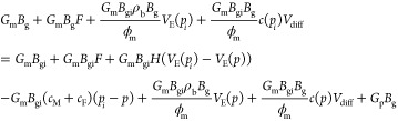B6

Organize and get the following formula:

B7

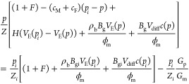
Divide both sides by G_mB_gi at the same time to get the following formula:

B8

As known,

B9

Substituting eq B9 into eq B8, the following formula can be obtained:

B10

Multiply both sides by at the same time to get the following formula:

B11

Substituting eq B9 into eq B11, the following formula can be obtained:

B12

Define the following expression:

B13

Substituting eq B13 into eq B12, the following formula can be obtained:

B14

As known,

B15

Substituting eq B15 into eq B14, the following formula can be obtained:

B16

As known,

B17

Substituting eq B17 into eq B13, the following formula can be obtained:

B18

Define the following expression:

B19

B20

B21

B22

B23

Substituting eqs B19, B20, B21, B22, and B23 into eq B18, the following formula can be obtained:

B24

B25

The pseudopressure can be expressed as:

B26

Differentiating eq B16 with respect to time, the following formula can be obtained:

B27

Then,

B28

B29

Substituting eqs B24 and B29 into eq B28, the following formula can be obtained:

B30

B31

B32

Equation B33 can be obtained from eqs 11 and 13 as follows:

B33

B34

B35

B36

Considering Langmuir isotherm adsorption, we obtain

B37

Differentiating the empirical formula for dissolved gases with respect to pressure, we obtain

B38

In the pseudosteady state, for variable flow/variable pressure, the material balance pseudotime is introduced:

B39

Calculate the integral of eq B30 and substitute eq B39 into eq B30:

B40

Substituting eq B15 into eq 40, we obtain

B41

By taking the derivative of eq B41, we obtain

B42

and

B43

Substituting eq B43 into eq B42, we obtain

B44

For a radius r, we obtain

B45

Assuming r_w ≪ r_e, from eqs B45 and B44, we obtain

B46

In the state of pseudosteady flow, considering the Darcy flow, we obtain

B47

Substituting eqs B17 and B26 into eq B47 and integrating eq B47, we obtain

B48

Assuming r_w ≪ r_e, we obtain

B49

and

B50

Substituting eq B49 into eq B50, we obtain

B51

Define the following expression:

B52

Substituting eq B52 into eq B51, we obtain

B53

Substituting eq B53 into eq B40, we obtain

B54

Substituting eq B54 into eq B41, we obtain

B55

Author Contributions

Y.Z. and Y.L. were involved in conceptualization and methodology preparation; M.Z. was involved in supervision; Z.B. was involved in data analysis; L.Y. was involved in data collection; and B.J. was involved in documentation.

The authors declare no competing financial interest.

References

- Ambrose R. J.; Hartman R. C.; Akkutlu I. Y.. Multi-component sorbed phase considerations for shale gas-in-place calculations. In SPE Production and Operations Symposium, 2011, 10.2118/141416-MS. [DOI] [Google Scholar]
- Hartman R. C.; Ambrose R. J.; Akkutlu I. Y.; Clarkson C. R.. Shale Gas-in-Place Calculations Part II—Multi-component Gas Adsorption Effects. In North American unconventional gas conference and exhibition, 2011, 10.2118/144097-MS. [DOI] [Google Scholar]
- Zhang Y.; Ju B.; Zhang M.; Wang C.; Zeng F.; Hu R.; Yang L. The effect of salt precipitation on the petrophysical properties and the adsorption capacity of shale matrix based on the porous structure reconstruction. Fuel 2022, 310, 122287 10.1016/j.fuel.2021.122287. [DOI] [Google Scholar]
- Lopez B.; Aguilera R.. Evaluation of quintuple porosity in shale petroleum reservoirs. In SPE Eastern Regional Meeting, 2013, 10.2118/165681-MS. [DOI] [Google Scholar]
- Orozco D.; Aguilera R.. A Material Balance Equation for Stress-Sensitive Shale Gas Reservoirs Considering the Contribution of Free, Adsorbed and Dissolved Gas. In SPE/CSUR Unconventional Resources Conference, 2015, 10.2118/175964-MS. [DOI] [Google Scholar]
- Zhang Y.; Yao S.; Zhang M.; Zhou X.; Mei H.; Zeng F. Prediction of adsorption isotherms of multicomponent gas mixtures in tight porous media by the oil–gas-adsorption three-phase vacancy solution model. Energy Fuels 2018, 32, 12166–12173. 10.1021/acs.energyfuels.8b02762. [DOI] [Google Scholar]
- Zhang Y.; Zhang M.; Mei H.; Ju B.; Shen J.; Ge L.; Zeng F.. Characterization of factors affecting the well deliverability of Longmaxi shale gas in the Jiaoshiba area by multivariate statistical analysis. In AICHE Annual Conference, 2020, 168750.
- Mengal S. A.; Wattenbarger R. A.. Accounting for adsorbed gas in shale gas reservoirs. In SPE middle east oil and gas show and conference, 2011, 10.2118/141085-MS. [DOI]
- Li Q.; Li P.; Pang W.; Li D.; Liang H.; Lu D. A new method for production data analysis in shale gas reservoirs. J. Nat. Gas Sci. Eng. 2018, 56, 368–383. 10.1016/j.jngse.2018.05.029. [DOI] [Google Scholar]
- King G. R. Material-balance techniques for coal-seam and devonian shale gas reservoirs with limited water influx. SPE Reservoir Eng. 1993, 8, 67–72. 10.2118/20730-PA. [DOI] [Google Scholar]
- Ahmed T. H.; Centilmen A.; Roux B. P.. A generalized material balance equation for coalbed methane reservoirs. In SPE annual technical conference and exhibition, 2006, 10.2118/102638-MS. [DOI] [Google Scholar]
- Firanda E.The development of material balance equations for coalbed methane reservoirs. In SPE Asia Pacific Oil and Gas Conference and Exhibition, 2011, 10.2118/145382-MS. [DOI] [Google Scholar]
- Penuela G.; Ordonez A.; Bejarano A.. A generalized material balance equation for coal seam gas reservoirs. In SPE Annual Technical Conference and Exhibition, 1998, 10.2118/49225-MS. [DOI] [Google Scholar]
- Moghadam S.; Jeje O.; Mattar L. Advanced gas material balance in simplified format. J. Can. Pet. Technol. 2011, 50, 90. 10.2118/139428-PA. [DOI] [Google Scholar]
- Mattar L.; McNeil R. The flowing gas material balance. J. Can. Pet. Technol. 1998, 37, PETSOC-98-02-06 10.2118/98-02-06. [DOI] [Google Scholar]
- Anderson D. M.; Mattar L. An improved pseudo-time for gas reservoirs with significant transient flow. J. Can. Pet. Technol. 2007, 46, PETSOC-07-07-05 10.2118/07-07-05. [DOI] [Google Scholar]
- Clarkson C. R.; Bustin R. M.; Seidle J. P. Production-data analysis of single-phase (gas) coalbed-methane wells. SPE Reservoir Eval. Eng. 2007, 10, 312–331. 10.2118/100313-PA. [DOI] [Google Scholar]
- Ambrose R. J.; Hartman R. C.; Diaz Campos M.; Akkutlu I. Y.; Sondergeld C.. New pore-scale considerations for shale gas in place calculations. SPE unconventional gas conference, 2010, 10.2118/131772-MS. [DOI] [Google Scholar]
- Wei M.; Duan Y.; Dong M.; Fang Q. Blasingame decline type curves with material balance pseudo-time modified for multi-fractured horizontal wells in shale gas reservoirs. J. Nat. Gas Sci. Eng. 2016, 31, 340–350. 10.1016/j.jngse.2016.03.033. [DOI] [Google Scholar]
- Zhang Y.; He Z.; Jiang S.; Lu S.; Xiao D.; Chen G.; Li Y. Fracture types in the lower Cambrian shale and their effect on shale gas accumulation, Upper Yangtze. Mar. Pet. Geol. 2019, 99, 282–291. 10.1016/j.marpetgeo.2018.10.030. [DOI] [Google Scholar]
- Dejam M.; Hassanzadeh H.; Chen Z. Semi-analytical solution for pressure transient analysis of a hydraulically fractured vertical well in a bounded dual-porosity reservoir. J. Hydrol. 2018, 565, 289–301. 10.1016/j.jhydrol.2018.08.020. [DOI] [Google Scholar]
- Zhang T.; Li Z.; Adenutsi C. D.; Lai F. A new model for calculating permeability of natural fractures in dual-porosity reservoir. Adv. Geo-Energy Res. 2017, 1, 86–92. 10.26804/ager.2017.02.03. [DOI] [Google Scholar]
- Connell L. D. A new interpretation of the response of coal permeability to changes in pore pressure, stress and matrix shrinkage. Int. J. Coal Geol. 2016, 162, 169–182. 10.1016/j.coal.2016.06.012. [DOI] [Google Scholar]
- Liu T.; Tang H.; Liu P.; Lin W.; Su G. Material balance equation and reserves calculation method for fractured closed shale gas reservoirs. Nat. Gas Explor. Dev. 2011, 34, 28–30. [Google Scholar]
- Wang D.; Guo P.; Chen H.; Fu W.; Wang Z.; Ding H. Deduction of material balance equation and reserves calculation for new adsorbed gas reservoirs. Lithol. Reservoirs 2012, 24, 83–86. [Google Scholar]
- Yang L.; Mei H.; Zhang M.; Yuan E.. Calculation method of shale gas reservoir reserves considering dissolved gas in kerogen. Xinjiang Pet. Geol. 2016, 05. [Google Scholar]
- Orozco D.; Aguilera R. A material-balance equation for stress-sensitive shale-gas-condensate reservoirs. SPE Reservoir Eval. Eng. 2017, 20, 197–214. 10.2118/177260-MS. [DOI] [Google Scholar]
- He L.; Mei H.; Hu X.; Dejam M.; Kou Z.; Zhang M. Advanced flowing material balance to determine original gas in place of shale gas considering adsorption hysteresis. SPE Reservoir Eval. Eng. 2019, 22, 1282–1292. 10.2118/195581-PA. [DOI] [Google Scholar]
- Meng Y.; Li M.; Xiong X.; Liu J.; Zhang J.; Hua J.; Zhang Y. Material balance equation of shale gas reservoir considering stress sensitivity and matrix shrinkage. Arabian .o Geosci. 2020, 13, 1–9. 10.1007/s12517-020-05485-6. [DOI] [Google Scholar]
- Williams-Kovacs J. D.; Clarkson C. R.; Nobakht M.. Impact of material balance equation selection on rate-transient analysis of shale gas. In SPE Annual Technical Conference and Exhibition, 2012, 10.2118/158041-MS. [DOI] [Google Scholar]
- Dejam M. Advective-diffusive-reactive solute transport due to non-Newtonian fluid flows in a fracture surrounded by a tight porous medium. Int. J. Heat Mass Transfer 2019, 128, 1307–1321. 10.1016/j.ijheatmasstransfer.2018.09.061. [DOI] [Google Scholar]
- Langmuir I. The adsorption of gases on plane surfaces of glass, mica and platinum. J. Am. Chem. Soc. 1918, 40, 1361–1403. 10.1021/ja02242a004. [DOI] [Google Scholar]
- Mehrotra A. K.; Svrcek W. Y. Correlations for properties of bitumen saturated with CO2, CH4 and N2, and experiments with combustion gas mixtures. J. Can. Pet. Technol. 1982, 21, PETSOC-82-06-05 10.2118/82-06-05. [DOI] [Google Scholar]
- Fetkovich M. J.Decline curve analysis using type curves. In Fall Meeting of the Society of Petroleum Engineers of AIME, 1973, 10.2118/4629-MS. [DOI] [Google Scholar]