Abstract
Objective:
Graphical deep learning models provide a desirable way for brain functional connectivity analysis. However, the application of current graph deep learning models to brain network analysis is challenging due to the limited sample size and complex relationships between different brain regions.
Method:
In this work, a graph convolutional network (GCN) based framework is proposed by exploiting the information from both region-to-region connectivities of the brain and subject-subject relationships. We first construct an affinity subject-subject graph followed by GCN analysis. A Laplacian regularization term is introduced in our model to tackle the overfitting problem. We apply and validate the proposed model to the Philadelphia Neurodevelopmental Cohort for the brain cognition study.
Results:
Experimental analysis shows that our proposed framework outperforms other competing models in classifying groups with low and high Wide Range Achievement Test (WRAT) scores. Moreover, to examine each brain region’s contribution to cognitive function, we use the occlusion sensitivity analysis method to identify cognition-related brain functional networks. The results are consistent with previous research yet yield new findings.
Conclusion and significance:
Our study demonstrates that GCN incorporating prior knowledge about brain networks offers a powerful way to detect important brain networks and regions associated with cognitive functions.
Index Terms—: Graph convolutional networks, functional magnetic resonance imaging, functional connectivity, brain functional networks, human cognition
I. Introduction
Functional magnetic resonance imaging (fMRI) measures blood-oxygen-level-dependent (BOLD) contrast signals to track the brain cells’ energy activity, providing a non-invasive, high-resolution way to analyze the brain statistical patterns. The human brain is a complex functional system, in which nerves communicate via trillions of connections. However, the brain regions can functionally interact with each other even in the absence of a direct anatomical connection [1]. To this end, functional connectivity (FC) [2]–[4], defined as temporal correlations of different regions of interest (ROIs), has been used to study human psychology and physical brain development. Meier et al. [5] analyzed FC networks built from resting-state fMRI to discriminate different age groups. Greene and Gao et al. [6], [7] showed that FC derived from task fMRI can be used for predicting fluid intelligence. Xiao et al. [8], [9] used FC derived from multiple paradigms of fMRI for intelligence quotient prediction. All these studies demonstrate that FC contains essential discriminative information for human cognitive trait prediction, measures of human brain maturation, and biomarker identification.
Recently, deep learning has gained attraction for FC studies [10]–[12] due to its power for feature representation. With massive parameters to optimize, deep learning models generally require large quantities of data. However, fMRI data is generally of a limited sample size to perform FC analysis because the data collection process is costly and time-consuming. In addition, the cognitive and psychiatric assessments conducted for subjects contain high evaluation errors and variance, increasing the difficulty in predictive tasks. To this end, the relationship between subjects can be explored as prior knowledge to improve the fitting of deep learning models. To incorporate both subject relationship information and FC of each subject, models based on graph theory [13], [14] are utilized.
In this paper, we propose a graph convolutional network (GCN) based framework to predict subjects’ cognition using FCs. Specifically, we build a subject-subject affinity graph for each fMRI paradigm, in which each node corresponds to one subject. The features of nodes are the FCs derived from the fMRI. Likewise, the edges between nodes represent the similarities of FCs between subjects, suggesting that each node can aggregate the information from neighbors. As a result, the labels on a small subset of nodes can be propagated through the whole graph to the unlabeled nodes. Then, GCN [15]–[18] is applied to the subject-subject graph to perform the classification task. Using the graph as the input, GCN can automatically extract features from each node and then aggregate them based on spatial structures of the graph via localized graph filters. As a result, semi-supervised graph embedding [19] is delivered, which uses both features on the nodes and topological structure of the graph. However, the over-smoothing issue limits the predictive performance and results in the overfitting problem for a small sample size, which has not been investigated by previous research [15]–[18]. We enforce a Laplacian regularization term [20] as an additional smoothness term on the embedding layer to address the over-smoothing issue. Besides, the effect of the different similarity functions is investigated, which directly constrains the input graph’s smoothness.
To validate our framework, we apply it to the Philadelphia Neurodevelopmental Cohort (PNC) [21] to study the brain mechanisms underlying human cognition. The Wide Range Achievement Test (WRAT) score [22], which measures an individual’s ability in reading, spelling, comprehending, and solving mathematical problems, is adopted as the measure of cognitive ability. We divide subjects into different groups based on their WRAT scores, and apply a semi-supervised GCN to perform the cognition level classification on the partial labeled subject-subject graph. Moreover, with the trained GCN model, we identify the significant brain networks underlying human cognition.
The main contributions of this paper are summarized as follows: 1) we propose a GCN based framework to incorporate subject-subject information and obtain superior performance for cognition classification using FC; 2) we alleviate the overfitting problem by enforcing a Laplacian regularization term; 3) the functional networks associated with human cognition are identified using the occlusion sensitivity method.
The remainder of this paper is structured as follows. We first present the proposed GCN model and the corresponding pipeline in Section II. We then conduct the experiments on the PNC dataset, including the comparison of performance with other models, parameter sensitivity studies, and brain functional network identification in Section III. We discuss some limitations with an outlook on future work in Section IV, followed by conclusion in Section V.
II. METHODOLOGY
In this section, we present the key components of our proposed GCN model and the corresponding pipeline.
A. Graph Convolutional Networks
As shown in Fig.1, the BOLD fMRI signal is first pre-processed and projected into the ROI time series according to the Power template [23]. A subject-subject affinity graph is then built using the ROI time series, in which is the set of nodes as , and is the set of edges, representing subject-subject relationships. Here, we assume the graph is weighted and undirected. The vectorized functional connectivity is regarded as the input feature calculated from the ROI time series for individuals, where d is the feature dimension. The Laplacian matrix , defined in Eq.1, is then used to represent the subject-subject graph, where is the adjacency matrix and A(i,j) represents the edge weight between subject i and subject j.
Fig. 1.
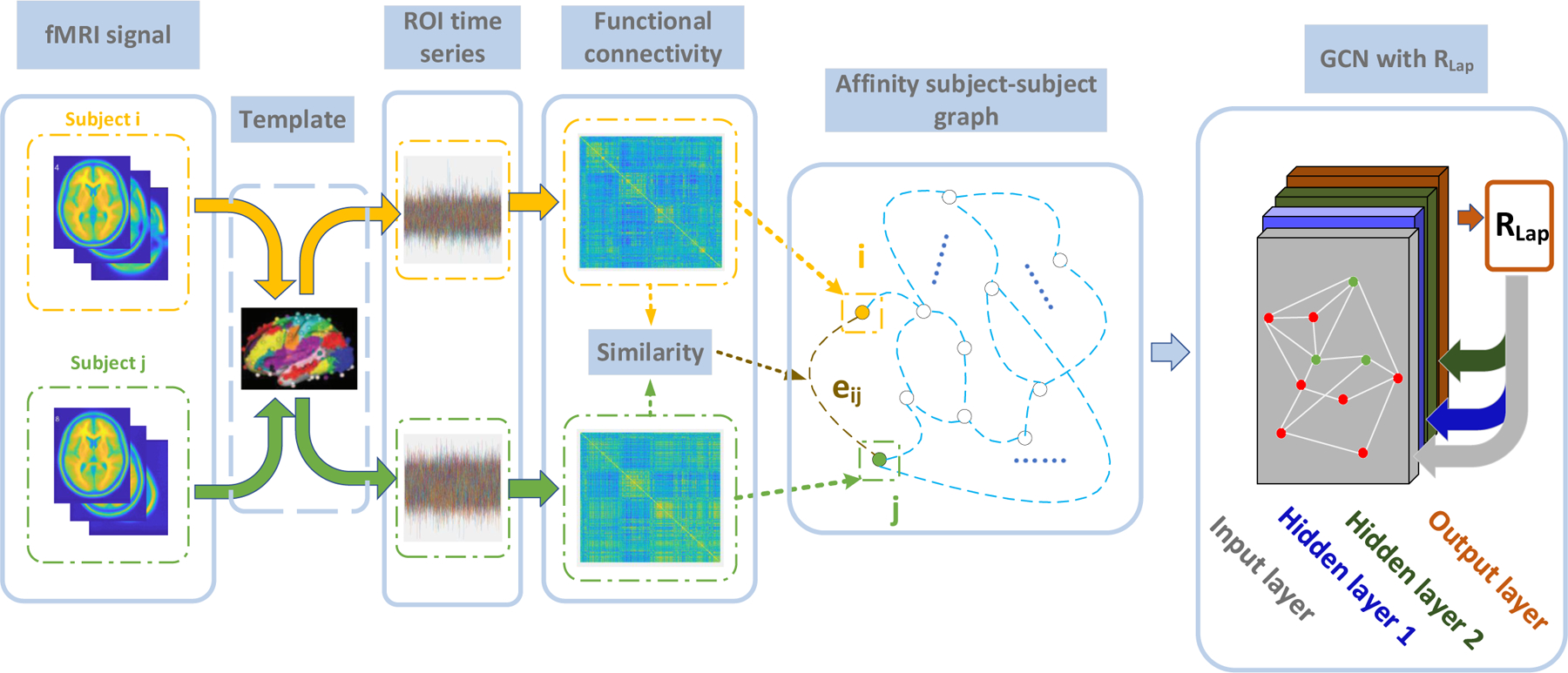
The flowchart of this study. First, the fMRI for each subject is mapped to the ROI time series using the Power brain template [23], followed by FC calculation via Pearson correlation. The affinity subject-subject graph is then built by measuring the similarity between FCs as edges, e.g., eij between node i and node j. Next, the GCN is applied for the classification of different cognitive functions. In this step, the graph is sparsified by K-nearest neighbors, and partially labeled (e.g., nodes with labels are marked in green, while nodes without labels are marked in red) for semi-supervised learning. The Laplacian regularization term RLap is enforced at the output layer, and the model parameters are estimated via back-propagation.
| (1) |
where D is the degree matrix, i.e., , and is the identity matrix. Graph Laplacian [24] is positive-semi-definite, whose eigendecomposition is
| (2) |
where Λ is a diagonal matrix whose diagonal elements are the eigenvalues of L, and U is the matrix of eigenvectors.
Graph convolution uses the eigenvectors of the Laplacian matrix L in Eq.1 as the bases of the graph spectrum. Accordingly, the graph convolutional networks [17], [25] are defined as
| (3) |
where H(l) is the feature representation at the lth hidden layer, and ϕ is the activation function.
The graph filter g is designed to incorporate the graph structure, which enables each node to aggregate the information from neighbors. It can be approximated as a truncated expansion in terms of polynomials in Eq.4 to reduce computational cost.
| (4) |
where θk is the weight of Λk. The Chebyshev polynomial approximation in Eq.5 is next utilized to reduce the number of parameters.
| (5) |
where λmax refers to the largest eigenvalue of L; is the kth order Chebyshev polynomial with k = 1, T0 = IN and . Therefore, the GCN layers [17] are simplified to
| (6) |
where , and W(l) and B(l) are the weight matrix and the bias matrix for the lth hidden layer, respectively. The weight and bias matrices are shared for all nodes, which can be learned with the labeled nodes and then tested on the unlabeled nodes.
B. Subject-subject graph analysis using semi-supervised GCN
Here we demonstrate the procedures by applying GCN to analyze the FCs derived from fMRI time series. Specifically, the FC of each subject is calculated by the Pearson correlation of pairwise ROIs. The FC of the ith subject is then vectorized to . The feature matrix of the graph can be defined as , where N is the total number of subjects.
The subject-subject affinity graph is then built as follows. The edges of the graph are defined as the similarity between the node features, which can capture the affinity relationship between subjects. Several similarity functions are considered including: the Gaussian similarity in Eq.7, the cosine similarity in Eq.8, and the median similarity [26] in Eq.9.
| (7) |
| (8) |
| (9) |
where xi and xj represent the feature vectors for node i and node j, respectively; β in Eq.7 is a scaling parameter; σ(xi) in Eq.9 is defined as the median of the distances between node i and its neighbors.
In addition, the K-nearest-neighbor (KNN) is applied to the adjacency matrix A before calculating in Eq.6. That is, only K most substantial connection edges are reserved, while the rest of the edges are set to zeros. In the process of graph convolution, some information aggregated from neighbors is simply noise, i.e., small correlation values are observed between the pair of nodes. KNN edge-selection significantly reduces the noise, resulting in increased sparsity of the graph. The graph is then partially labeled for semi-supervised learning. Specifically, the GCN is applied to learn the embedding of the nodes first. The weight matrix W(l) and the bias matrix B(l) of each GCN layer learned through the labeled nodes for training are then shared with unlabeled nodes during testing.
C. Laplacian regularization term
GCN aggregates the information of neighboring nodes via mean pooling. This recursive local smoothing raises the risk of over-smoothing, i.e., the embeddings of connected nodes with a larger edge weight tend to be more similar. Therefore, a Laplacian regularization term RLap is enforced in Eq.10.
| (10) |
where is the embedding output of the nodes, L is the Laplacian matrix in Eq.1, and A is the adjacency matrix before applying KNN. The Laplacian regularization term, enforced at the output layer of GCN, can smooth the embedding results over the whole graph and reduce the variations in the graph. This regularization is applied to both labeled and unlabeled nodes. Besides the Laplacian regularization term, the l2 regularization term is also enforced.
For the semi-supervised classification task, the loss function is defined by cross entropy balanced with the regularization terms, shown in Eq.11.
| (11) |
where is the set of labeled nodes, and , between 0 and 1, is the embedding value of nodes. F(= 2) represents the number of classes, and λ1 and λ2 are the parameters for RLap and , respectively.
III. Experiment
In the experiment, we examined the relationship between human cognitive ability and brain connectivity networks by applying the proposed framework to the analysis of PNC data. Multiple studies, including accuracy comparison, parameter sensitivity studies, and brain functional network identification, demonstrated the effectiveness of the proposed GCN model.
A. PNC data
The brain fMRI datasets from the PNC were used for the experiment. The data includes three paradigms of fMRI: resting-state fMRI (rest-fMRI), emotion task fMRI (emoid-fMRI), and nback state fMRI (nback-fMRI) (collected from 975 subjects). All BOLD scans were acquired on a single 3T Siemens TIM Trio whole-body scanner with a single-shot, interleaved multi-slice, gradient-echo, echo-planar imaging sequence. The total scanning time was 50 minutes, 32 seconds, with a voxel resolution of 3 × 3 × 3 mm with 46 slices. The imaging parameters were set to achieve whole brain coverage (i.e., TR = 3000 ms, TE = 32 ms, and flip angle = 90 degrees) [21]. Gradient performance was 45 mT/m, with a maximum slew rate of 200 T/m/s. The rest-fMRI scan duration was 6.2 minutes (124 TR), during which subjects were asked to stay still and keep awake with eyes open. The duration of emoid-fMRI scan was 10.5 minutes (210 TR), during which subjects were asked to view faces displaying different emotions, e.g., angry, sad, fearful, happy, and to label the emotion type of the face. The nback-fMRI scan duration was 11.6 minutes (231 TR), during which subjects were asked to conduct n-back memory tasks, which indicated the ability of lexical processing and working memory. In our experiment, the WRAT scores were used as cognitive assessments to investigate the relationship between FCs and human cognitive abilities. The WRAT distributions of tested subjects for each of three paradigms of fMRI are shown in the Fig.3. The numbers of subjects, as shown in Fig.2, were 910 (nback-fMRI), 680 (emoid-fMRI), and 878 (rest-fMRI), respectively.
Fig. 3.
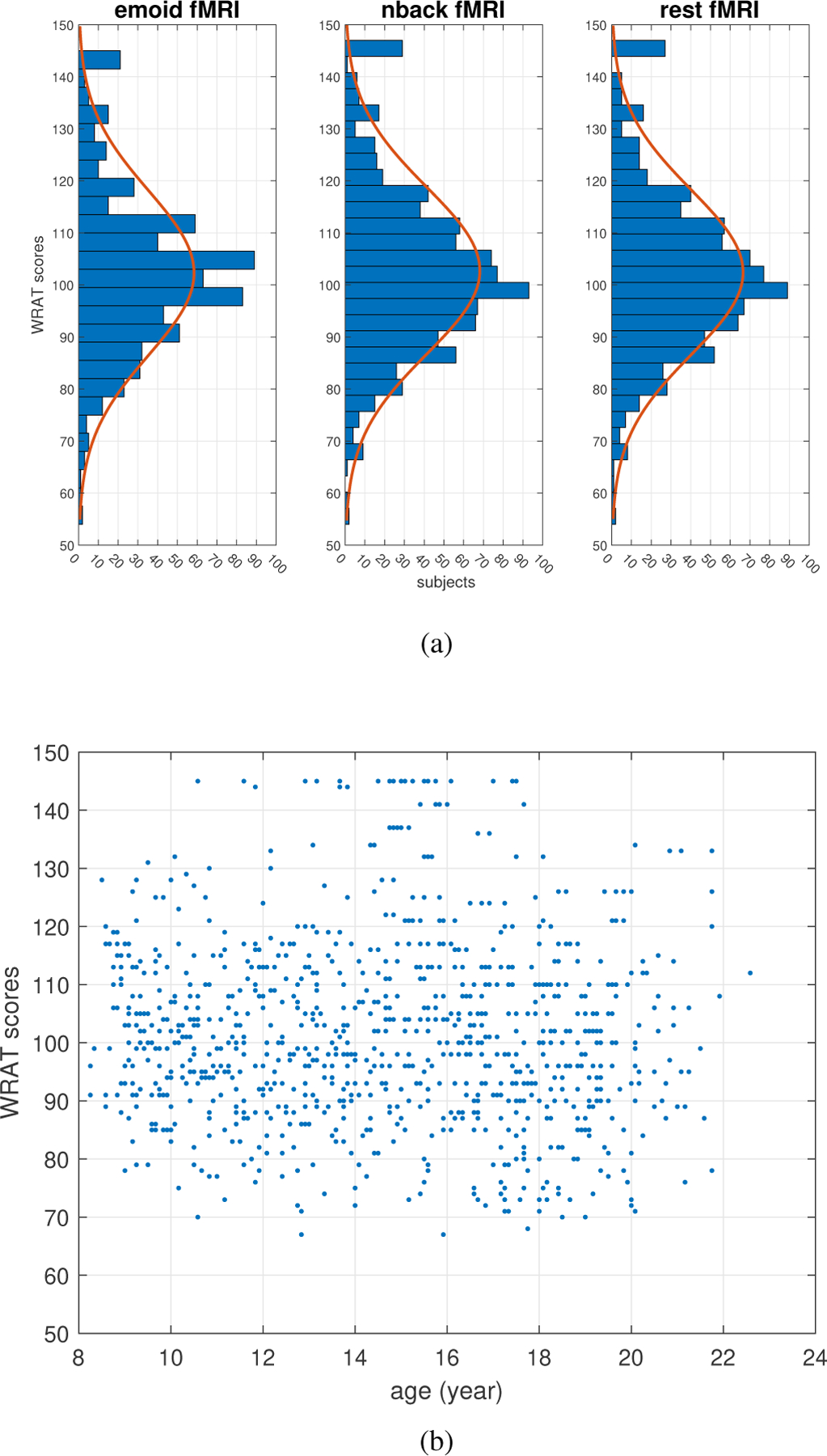
(a) The WRAT score distributions of tested subjects for three paradigms of fMRI; (b) The age-WRAT scatter plot for all subjects
Fig. 2.
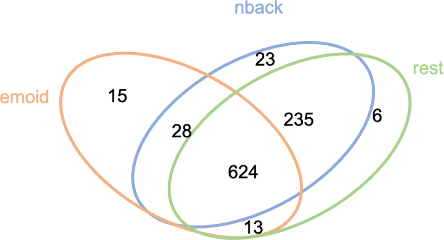
The Venn diagram of the number of subjects for three fMRI paradigms
SPM12 1 was used to conduct motion correction, spatial normalization, and smoothing with a 3mm Gaussian kernel. Multiple regressions were used to remove the influence of motion [27]. As a result, 264 ROIs were obtained (containing 21,384 voxels) using the Power template (sphere radius of the ROI was 5mm) [23]. Potential confounders (age, gender, head motion) for WRAT and fMRI association were explored.
Age: The WRAT-age distribution was shown in Fig. 3 (b). The standardized WRAT scores [22] were considered, for which the grade and age norms were enforced to control the age factor for the WRAT scores calibration.
Gender: The gender-WRAT information was shown in Table I. Since the mean and standard deviation of WRAT scores for males and females were close, the gender effects on WRAT classification were ignorable.
Head motion: 6 rigid body motion parameters (3 translations , and 3 rotations at time step i) were collected as a vector . The framewise displacement (FD) [28] shown in Eq.12 was then calculated.
TABLE I.
Gender-WRAT information.
| property\group | male | female | Total |
|---|---|---|---|
| number of subjects | 463 | 512 | 975 |
| mean WRAT scores | 102.927 | 100.891 | 101.857 |
| std WRAT scores | 16.572 | 14.745 | 15.664 |
| (12) |
Using Pearson correlation coefficients, we further tested the hypothesis that there was no relationship between the WRAT scores and the mean FD over time. The p-values were 0.3029 for emoid-fMRI, 0.3599 for nback-fMRI, and 0.1785 for rest-fMRI, respectively. No significant relationships between FD and WRAT scores were observed at 0.05 level.
Next, the top 20% and the bottom 20% of the subjects from each fMRI paradigm were grouped as high and low WRAT cognitive groups. Accordingly, 268, 356, and 342 subjects for emoid-fMRI, nback-fMRI, and rest-fMRI were selected, respectively. The affinity graphs were built separately for each paradigm. The principal component analysis was used for all three paradigms to reduce the dimension of node features. The number of components was selected such that 90% of the total variance was explained, resulting in 165, 214, 224 components remained for the emoid-fMRI, nback-fMRI, and rest-fMRI, respectively. We repeated the experiments with different ratios between unlabelled and labelled nodes. The ratios of labeled nodes used for training and validation ranged from 30% to 70% in increments of 5%. No significant improvements of classification performance for testing were observed after using more than 50% of the subjects for training and validation.
B. Experiment set-up
We randomly selected 50% of nodes from each group to be labeled (1 for high WRAT score and 0 for low WRAT score). For each experiment, 10% of these labeled nodes (5% of total) were regarded as validation dataset, and the rest 90% were used for training. The FCs derived from different paradigms were used as the node features. The classification accuracy was evaluated on the unlabeled nodes. The ADAM optimizer [29] was used for optimization. The hyperparameters of GCN, including the number of layers, the number of channels in each layer, activation function for each layer, learning rate, learning rate decay, epochs number, the trade-off parameters of L2 and the Laplacian regularization term, were tuned via random search [30]. The results were shown in Table.II. The models were trained on the computer with an Intel(R) Core™ i7–8700K Processor, a 16G RAM, and a NVIDIA GeForce GTX 1080 GPU, 8G RAM. The training time was recorded to document the complexity of the models. Bootstrapping analysis was utilized to evaluate the performance of the models, which reduced the effect of sampling bias via 10 repeated experiments. We randomly split the nodes into training, validation, and test sets for each repeated experiment. Then the means and standard deviations of the accuracy were reported and compared for different models. Specifically, pairwise t-test comparisons were performed between the results of our method and the other competing approaches. Next, p-values were reported to demonstrate if significant improvement of the predictive performance was observed.
TABLE II.
The default hyperparameters.
| Hyperparamter | Value |
|---|---|
| Network architecture (channels) | [1024, 512, 512, 1] |
| Activation function | [ReLu, ReLu, ReLu, Sigmoid] |
| Similarity Function | Gaussian |
| Maximum Epochs | 5000 |
| Learning Rate | 1e-5 |
| Optimizer | ADAM |
| λ1 ( parameter) | 1e-4 |
| λ2 (RLap parameter) | 0.005 |
| Learning rate exponential decay | 0.9/1000 epochs |
In the experiment, we found that more layers (e.g., 4 or 5 hidden layers) did not significantly improve the performance. In contrast, setting more than 3 layers increased the chance of over-smoothing. This was consistent with the conclusion in [31] that more stacked layers of GCN would not help the final results for limited labeled datasets.
C. Hyperparameter selection
Hyperparameter selection can influence the topological graph structures. Therefore, the selection of these hyperparameters (K for KNN, and similarity function ) was further investigated.
1). KNN parameter:
The selection on the number of the nearest neighbors K impacts the sparsity level of the graph. In the experiment, K was set to 10, 20, compared to the fully connected graph (K = N − 1). Gaussian similarity in Eq.7 was utilized. The parameter of the Laplacian regularization term was set to 0. The classification results on emoid-fMRI and nback-fMRI with different values of K were shown in Fig.4. The model frequently failed to converge when setting K = 10 and K = N − 1 for rest-fMRI. The classification accuracy was 0.658 ± 0.012 for K = 20 using rest-fMRI. Based on the experiment, we found that the optimization of the model will be challenging with the observed overfitting. However, enforcing the Laplacian regularization term helped to solve the problem.
Fig. 4.
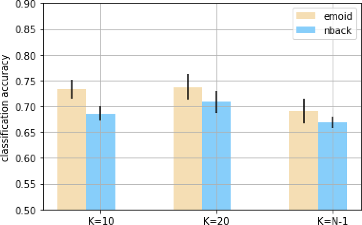
The accuracy of classification for different K on emoid-fMRI and nback-fMRI
2). Similarity function selection:
The use of different similarity function can have an effect on the weight distribution of the connected edges. Three frequently used similarity functions (the Gaussian similarity in Eq.7, the cosine similarity in Eq.8, and the median similarity in Eq.9) were compared. K for KNN was set to 20. The parameter of the Laplacian regularization term was set to 0. The rest of the hyperparameters were set to the default values.
From the results in Table III, the models with Gaussian similarity outperformed those with the cosine similarity and the median similarity. The median similarity function further smoothed the graph, which could worsen the over-smoothness problem if not properly used [31], [32]. The edge weights calculated using Gaussian similarity are more discriminative, as shown in Fig.6, which resulted in better predictive performance. Therefore, the Gaussian similarity was chosen in this work to evaluate the performance of the GCN.
TABLE III.
The classification results for different similarity functions.
| Function | Emoid | Nba | ck | Rest | ||
|---|---|---|---|---|---|---|
| Accuracy | p-value | Accuracy | p-value | Accuracy | p-value | |
| Gaussian | 0.737 ± 0.025 | - | 0.709 ± 0.018 | - | 0.667 ± 0.019 | - |
| Cosine | 0.722 ± 0.019 | 0.1502 | 0.616 ± 0.022 | 5.8012e-09 | 0.574 ± 0.014 | 2.2382e-10 |
| Median | 0.579 ± 0.029 | 3.0576e-10 | 0.544 ± 0.013 | 6.0731e-15 | 0.543 ± 0.014 | 2.5488e-12 |
Fig. 6.
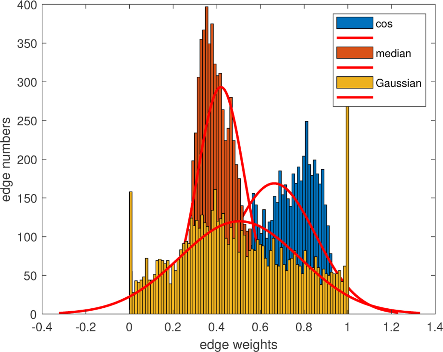
Edge distributions using different similarity functions
3). Regularization and visualization:
The overfitting issue was observed for the GCN model as shown in Fig.5 (a). The Laplacian regularization was thus applied. The parameter of the Laplacian regularization was tuned using random search between 0.1 and 0.001, with the best value found to be 0.005. With the Laplacian regularization term, the gap between the training and testing accuracy decreased significantly. In addition, higher classification accuracy was also observed via adding the Laplacian regularization term, shown in Table IV.
Fig. 5.
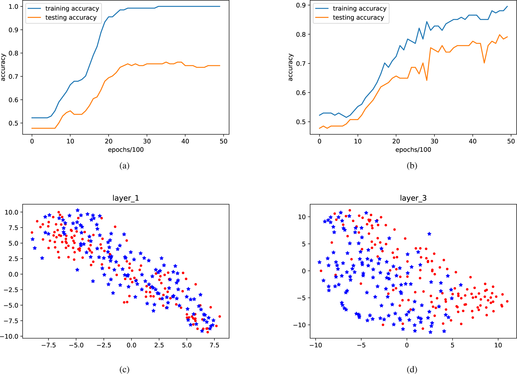
(a) An example of the overfitting, where a large gap (around 27%) can be observed between training and testing accuracy. (b) Both the training and testing accuracy after the Laplacian regularization term is applied. The overfitting problem is thus alleviated. Figures (c) (d) are the visualization of GCN trained on rest-fMRI, in which red dots represent subjects with high WRAT scores, and blue asterisks represent subjects with low WRAT scores. From the first layer to the third layer of GCN, two groups are observed to be clustered more discriminatively.
TABLE IV.
The classification results with different models.
| Model | Emoid | Nback | Rest | |||
|---|---|---|---|---|---|---|
| Accuracy | p-value | Accuracy | p-value | Accuracy | p-value | |
| PCA+SVM | 0.555 ± 0.011 | 2.100e-16 | 0.558 ± 0.016 | 1.010e-15 | 0.567 ± 0.013 | 2.562e-13 |
| DM+SVM | 0.596 ± 0.033 | 4.862e-11 | 0.580 ± 0.001 | 2.635e-16 | 0.553 ± 0.008 | 3.073e-15 |
| PCA+SRC | 0.567 ± 0.035 | 9.458e-12 | 0.545 ± 0.018 | 9.380e-16 | 0.560 ± 0.013 | 7.209e-14 |
| PCA+DT | 0.566 ± 0.030 | 1.418e-12 | 0.581 ± 0.013 | 1.733e-15 | 0.579 ± 0.016 | 6.359e-12 |
| PCA+MLP | 0.707 ± 0.0370 | 5.729e-04 | 0.707 ± 0.020 | 5.840e-04 | 0.662 ± 0.019 | 0.004 |
| PCA+GCN* | 0.737 ± 0.025 | 0.0175 | 0.709 ± 0.018 | 3.8126e-04 | 0.667 ± 0.019 | 0.01 |
| PCA+GCN | 0.765 ± 0.021 | - | 0.742 ± 0.015 | - | 0.689 ± 0.016 | - |
The t-distributed stochastic neighbor embedding (t-SNE) was utilized to visualize the GCN via mapping the high dimensional data to a 2D space. The results of the input layer and the last hidden layer of GCN were shown in Fig.5. In the figure, the nodes were observed to be clustered into two classes. From Fig.5 (c) (d), the two clusters were observed to be more discriminative from the input layer to the last hidden layer.
D. Model performance evaluation
1). Running time comparison:
Multiple epochs were trained for deep learning models. Therefore, multi-layer perceptron (MLP) network with an equal number of hidden layers and equal number of neurons in each layer was compared with GCN to evaluate the complexity. The average running time for 100 epochs was 6.92s for MLP and 7.43s for GCN, respectively. GCN spent around 7.3% more time than MLP.
2). Model comparison:
The performance of GCN was evaluated on the PNC dataset. The FCs derived from emoid-fMRI, nback-fMRI, and rest-fMRI were used as raw inputs, respectively. The same dataset splitting strategy was applied:
45% samples were used for training.
5% samples were used for validation.
50% samples were used for testing.
The dataset was divided without bias regarding different groups into different classes. The principal components analysis (PCA) was next applied to avoid out-of-memory. Bootstrapping analysis was used to evaluate the classification performance. The two-sample t-test between the competing model and GCN was performed using 10 repeated experiments. The dataset splitting and model training procedure was repeated for each experiment, after which the mean and standard deviation of the accuracy was recorded. The GCN was compared with following models:
PCA+SVM: performing PCA followed by classification via Support Vector Machine (SVM).
DM+SVM: performing diffusion map (DM) [33] followed by classification via SVM.
PCA+SRC: performing PCA followed by classification via sparse representation coding (SRC) [34].
PCA+DT: performing PCA followed by classification via decision tree classifier (DT).
PCA+MLP: performing PCA followed by classification via MLP, the neuron network structure of which was identical to GCN.
PCA+GCN*: performing PCA followed by classification via GCN without the use of the Laplacian regularization term.
We tuned the penalty parameter C of the SVM within the range of {10−3,10−2,10−1,1,10} and found the linear kernel resulted in better classification performance for PCA and DM. The target dimension varied within the range of {10,20,…,100} in the DM. The criterion was set to be Gini impurity in the DT and the l1 parameter of SRC was tuned within the range of {10−5,10−4,10−3,10−2,10−1}. As can be seen, SVM, SRC, and DT, yielded significantly lower accuracy than the deep learning models, e.g., MLP and GCN. The groups can be better discriminated by task fMRI (emoid-fMRI and nback-fMRI) than by rest-fMRI when the neural networks (MLP and GCN) were used. In addition, GCN without the Laplacian regularization term still outperformed the MLP and its performance can be further improved via enforcing the Laplacian regularization term.
E. Result analysis
From the results about hyperparameter selection, using 20 nearest neighbors and Gaussian similarly function was the best choice. Because of the overfitting problem on the small sample dataset, as shown in Fig.5 (a), the Laplacian regularization term was enforced. Fig.5 (b) showed that the gap between training and testing accuracy become narrower after enforcing the Laplacian regularization term. In particular, the t-SNE mapping in Fig.5(c) and (d) showed that GCN learned an embedding map, based on which the subjects can be better clustered into different groups.
The performance of GCN was compared to that of other classifiers in Section III-D2. Results in Table IV demonstrate superior performance of GCN over other conventional models. Even GCN without the Laplacian regularization term still outperformed the MLP with the same network structure. This experimental result supports our argument that the classification performance can be enhanced by incorporating the subject-subject relationship information.
F. Brain functional network identification via occlusion sensitivity analysis
Occlusion sensitivity (OS) [35], [36] can be used to visualize and understand the neuron networks via tracking the activation parts of the input features. This approach was applied to identify relevant brain functional networks. From the results summarized in Table IV, the emoid-fMRI was shown to better classify different WRAT groups than other paradigms of fMRI. As a result, FC derived from the emoid-fMRI was used to identify critical networks. To be specific, first, the parameters (e.g., the weights of the hidden layers and the correlation matrix for PCA) of 10 trained GCN were fixed. The FCs derived from emoid-fMRI on individual brain functional networks were then zero-out, which simulated the situation when a specific brain network was not working correctly. 10 GCN models were then tested using different region-blocked FC matrices. Thus, brain functional networks that played essential roles were inferred. Since brain functional networks differ in size, the ROI-level average sensitivity, defined as the OS of the brain functional network divided by the number of ROIs in the network, was also measured. Accordingly, SM, CNG, AUD, DMN, which play essential roles in WRAT classification, were identified, as shown in Fig.7. Besides, memory retrieval network (MEM), ventral attention (VTRL), and cerebellum (CB) were observed with high ROI-level average OS. The visualization results are shown in Fig.8.
Fig. 7.
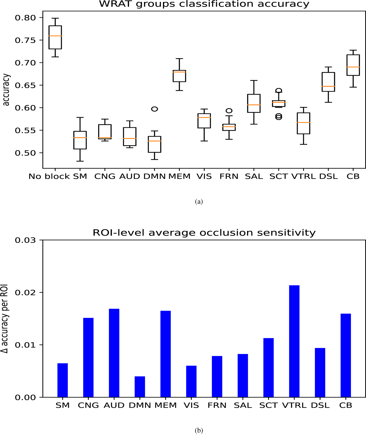
The classification accuracy on FC derived from emoid-fMRI in different functional-network-blocked cases. The models were tested under the condition that a particular brain functional network was blocked. The full names of brain functional networks are: no brain functional networks were blocked (No block), sensorimotor network (SM) with 35 ROIs, cingulo-opercular task control (CNG) with 14 ROIs, auditory network (AUD) with 13 ROIs, default mode network (DMN) with 58 ROIs, memory retrieval network (MEM) with 5 ROIs, visual network (VIS) With 31 ROIs, Fronto-parietal Task Control (FRN) with 25 ROIs, salience network (SAL) with 18 ROIs, subcortical network (SCT) with 13 ROIs, ventral attention (VTRL) with 9 ROIs, dorsal attention (DSL) with 11 ROIs, cerebellum (CB) with 4 ROIs.(a) describes the result of the accuracy alteration via blocking specific brain functional network, and (b) shows the ROI-level average occlusion sensitivity in the specific brain functional network.
Fig. 8.
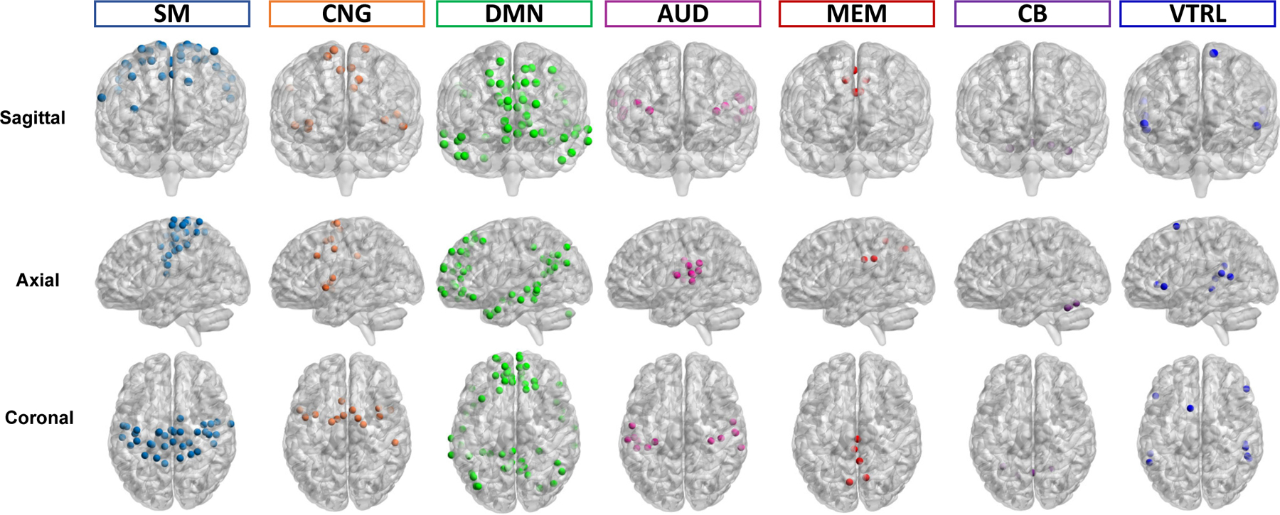
The brain functional networks identified with ROI-level average OS in sagittal, axial, and coronal views, respectively, including SM, CNG, DMN, AUD, MEM, VTRL, and CB. Dots with different colors represent ROIs in different brain functional networks.
IV. Discussion
GCN is an ideal model to extract essential information from a network. In particular, we can incorporate both the node features and between-node relationships into the GCN. We investigated the application of GCN to the fMRI dataset with a small sample size. The experimental results in Section III showed that GCN can achieve superior classification accuracy than several competing models.
A. Brain functional network identification via GCN
We applied GCN to analyze the relationship between specific brain functional networks and cognitive functions. The OS of each brain functional network was explored. In particular, four brain functional networks were identified, including SM, CNG, AUD, and DMN.
SM: according to the study in [37]–[39], SM plays a critical role in various cognitive functions, such as verbal creativity, memory retrieval, imaginative process, and feedback-based control of vocal pitch.
CNG: a downstream role for CNG is observed, which involves cognitive control and maintaining cognitive functions available for current processing [40], [41].
AUD: study in [42] reveals that attention and cognitive control networks can be identified via the auditory discrimination task. However, little evidence on the direct relationship between AUD and human cognitive ability can be found.
DMN: the largest brain functional network, which contains more connections with other brain regions. Results from previous research [37], [43]–[45] show that DMN closely associates with ongoing cognition for goaldirected and goal-irrelevant task.
Interestingly, MEM, VTRL, and CB were discovered to deliver high ROI-level average OS. Particular ROIs with high ROI-level average OS, which were located in the brain functional networks with low OS, may still function critically in human cognition.
MEM: memory is part of the general human cognitive standard, which is closely related to the ability of various tasks [46]. In the experiment, WRAT scores were used to measure human cognitive ability, which impacts the academic ability of a subject. This measurement may result in MEM network to be underestimated.
VTRL: VTRL are positively correlated with various other brain regions, e.g., resting-state DMN network [44], [47]. Reports in [48], [49] reveal the recruitment of these areas under cognitive loading conditions.
CB: CB is believed to play an essential role in movement control. Studies in [50] [50], [51] suggest that CB also contributes to the cognitive functions of language, attention, and the response of fear or pressure.
These results uncover the relationship between brain functional networks and human cognitive function, which are consistent with previous findings.
B. Limitations and future work
Despite the success, our work still has the following limitations. First, our analysis relies on the assumption on static FC, without accounting for time-varying functional information [52]. Second, the PCA was applied to reduce the computational complexity of our model from to , where N is the number of subjects, Q = 264 is the number of ROIs, and d is the dimension of the feature vector. However, from the results of our previous work [53], the classification accuracy of SVM without PCA on rest-fMRI FC was comparable to that of MLP, and the use of PCA can cause a decrease in classification accuracy. A balance between computational complexity and classification accuracy should be further explored. Third, currently we performed classification based on FCs derived from each fMRI paradigm separately; it would be more helpful by using the integrated FCs as the inputs for the GCN model. Besides, the standard template used in SPM was derived from the adults, which may have limitations when applying to children subjects. The use of the templates for different ages deserves further study while beyond the scope of current focus.
V. Conclusion
This paper proposed a GCN based framework to extract fruitful information from brain FCs, which was used to study the brain-cognition relationship. We simultaneously incorporated the information of FC from each subject and between different subjects as prior knowledge. The Laplacian regularization term was enforced to overcome the overfitting problem when only a small size of sample is available. We validated the framework by classifying subject groups with high and low WRAT scores using real data from the PNC study. Through the experiment, GCN outperformed other conventional approaches with a classification accuracy of 76.5%, 74.2%, 68.9% for emoid-fMRI, nback-fMRI, and rest-fMRI, respectively. The superior classification accuracy demonstrates that incorporating the relationship between subjects can improve the fitting of the GCN model to real data. Furthermore, four important functional networks with the brain, including SM, CNG, AUD, and DMN, were identified via occlusion sensitivity analysis, which play critical roles in human cognitive functions. The results were consistent with the previous studies [9], [36], [54], [55]. In addition, specific brain regions or ROIs were identified, which may significantly contribute to human cognition. Therefore, these results demonstrate that the proposed GCN framework provides a valuable way for brain-cognition studies.
Acknowledgments
This work was supported in part by NIH under Grants R01 GM109068, R01 MH104680, R01 MH107354, P20 GM103472, R01 REB020407, R01 EB006841, 2U54MD007595, and in part by NSF under Grant #1539067.
Footnotes
Contributor Information
Gang Qu, Department of Biomedical Engineering, Tulane University, New Orleans, LA, 70112.
Wenxing Hu, Department of Biomedical Engineering, Tulane University, New Orleans, LA, 70112.
Li Xiao, School of Information Science and Technology, University of Science and Technology of China, Hefei, Anhui 230052, China.
Junqi Wang, Department of Biomedical Engineering, Tulane University, New Orleans, LA, 70112.
Yuntong Bai, Department of Biomedical Engineering, Tulane University, New Orleans, LA, 70112.
Beenish Patel, Department of Biomedical Engineering, Tulane University, New Orleans, LA, 70112.
Kun Zhang, Department of Computer Science, Xavier University of Louisiana, New Orleans, LA, 70125.
Yu-Ping Wang, Department of Biomedical Engineering, Tulane University, New Orleans, LA, 70112.
References
- [1].Damoiseaux JS and Greicius MD, “Greater than the sum of its parts: a review of studies combining structural connectivity and resting-state functional connectivity,” Brain structure and function, vol. 213, no. 6, pp. 525–533, 2009. [DOI] [PubMed] [Google Scholar]
- [2].Allen EA et al. , “Tracking whole-brain connectivity dynamics in the resting state,” Cerebral cortex, vol. 24, no. 3, pp. 663–676, 2014. [DOI] [PMC free article] [PubMed] [Google Scholar]
- [3].Calhoun VD et al. , “The chronnectome: time-varying connectivity networks as the next frontier in fmri data discovery,” Neuron, vol. 84, no. 2, pp. 262–274, 2014. [DOI] [PMC free article] [PubMed] [Google Scholar]
- [4].Yu Q et al. , “Modular organization of functional network connectivity in healthy controls and patients with schizophrenia during the resting state,” Frontiers in systems neuroscience, vol. 5, p. 103, 2012. [DOI] [PMC free article] [PubMed] [Google Scholar]
- [5].Meier TB et al. , “Support vector machine classification and characterization of age-related reorganization of functional brain networks,” Neuroimage, vol. 60, no. 1, pp. 601–613, 2012. [DOI] [PMC free article] [PubMed] [Google Scholar]
- [6].Greene AS et al. , “Task-induced brain state manipulation improves prediction of individual traits,” Nature communications, vol. 9, no. 1, pp. 1–13, 2018. [DOI] [PMC free article] [PubMed] [Google Scholar]
- [7].Gao S et al. , “Task integration for connectome-based prediction via canonical correlation analysis,” in 2018 IEEE 15th International Symposium on Biomedical Imaging (ISBI 2018). IEEE, 2018, pp. 87–91. [Google Scholar]
- [8].Xiao L et al. , “Multi-hypergraph learning-based brain functional connectivity analysis in fmri data,” IEEE Transactions on Medical Imaging, vol. 39, no. 5, pp. 1746–1758, 2020. [DOI] [PMC free article] [PubMed] [Google Scholar]
- [9].Xiao L et al. , “A manifold regularized multi-task learning model for IQ prediction from two fmri paradigms,” IEEE Transactions on Biomedical Engineering, vol. 67, no. 3, pp. 796–806, 2019. [DOI] [PMC free article] [PubMed] [Google Scholar]
- [10].Meszlényi RJ et al. , “Resting state fmri functional connectivity-based classification using a convolutional neural network architecture,” Frontiers in Neuroinformatics, vol. 11, p. 61, 2017. [Online]. Available: 10.3389/fninf.2017.00061 [DOI] [PMC free article] [PubMed] [Google Scholar]
- [11].Suk H-I et al. , “State-space model with deep learning for functional dynamics estimation in resting-state fmri,” NeuroImage, vol. 129, pp. 292–307, 2016. [Online]. Available: http://www.sciencedirect.com/science/article/pii/S1053811916000100 [DOI] [PMC free article] [PubMed] [Google Scholar]
- [12].Heinsfeld AS et al. , “Identification of autism spectrum disorder using deep learning and the abide dataset,” NeuroImage: Clinical, vol. 17, pp. 16–23, 2018. [Online]. Available: http://www.sciencedirect.com/science/article/pii/S2213158217302073 [DOI] [PMC free article] [PubMed] [Google Scholar]
- [13].Jie B et al. , “Topological graph kernel on multiple thresholded functional connectivity networks for mild cognitive impairment classification,” Human Brain Mapping, vol. 35, no. 7, pp. 2876–2897, 2014. [Online]. Available: 10.1002/hbm.22353 [DOI] [PMC free article] [PubMed] [Google Scholar]
- [14].Wang J et al. , “Functional network estimation using multigraph learning with application to brain maturation study,” Human brain mapping, vol. 42, no. 9, pp. 2880–2892, 2021. [DOI] [PMC free article] [PubMed] [Google Scholar]
- [15].Kazi A et al. , “Self-attention equipped graph convolutions for disease prediction,” in 2019 IEEE 16th International Symposium on Biomedical Imaging (ISBI 2019), 2019, pp. 1896–1899. [Google Scholar]
- [16].Parisot S et al. , “Disease prediction using graph convolutional networks: Application to autism spectrum disorder and alzheimer’s disease,” Medical Image Analysis, vol. 48, pp. 117–130, 2018. [Online]. Available: http://www.sciencedirect.com/science/article/pii/S1361841518303554 [DOI] [PubMed] [Google Scholar]
- [17].Kipf TN and Welling M, “Semi-supervised classification with graph convolutional networks,” international conference on learning representations, 2017. [Google Scholar]
- [18].Zitnik M et al. , “Modeling polypharmacy side effects with graph convolutional networks,” Bioinformatics, vol. 34, no. 13, pp. i457–i466, 2018. [DOI] [PMC free article] [PubMed] [Google Scholar]
- [19].Shi X et al. , “Graph temporal ensembling based semi-supervised convolutional neural network with noisy labels for histopathology image analysis,” Medical image analysis, vol. 60, p. 101624, 2020. [DOI] [PMC free article] [PubMed] [Google Scholar]
- [20].Belkin M et al. , “Manifold regularization: A geometric framework for learning from labeled and unlabeled examples,” Journal of machine learning research, vol. 7, no. Nov, pp. 2399–2434, 2006. [Google Scholar]
- [21].Satterthwaite TD et al. , “Neuroimaging of the philadelphia neurodevelopmental cohort,” Neuroimage, vol. 86, pp. 544–553, 2014. [DOI] [PMC free article] [PubMed] [Google Scholar]
- [22].Wilkinson G and Robertson G, “Wide range achievement test 4 professional manual: Psychological assessment resources,” 2006. [Google Scholar]
- [23].Power JD et al. , “Functional network organization of the human brain,” Neuron, vol. 72, no. 4, pp. 665–678, 2011. [DOI] [PMC free article] [PubMed] [Google Scholar]
- [24].Belkin M and Niyogi P, “Laplacian eigenmaps and spectral techniques for embedding and clustering,” in Advances in neural information processing systems, 2002, pp. 585–591. [Google Scholar]
- [25].Defferrard M et al. , “Convolutional neural networks on graphs with fast localized spectral filtering,” in Advances in neural information processing systems, 2016, pp. 3844–3852. [Google Scholar]
- [26].Zhu W et al. , “Ldmnet: Low dimensional manifold regularized neural networks,” in 2018 IEEE/CVF Conference on Computer Vision and Pattern Recognition, 2018, pp. 2743–2751. [Google Scholar]
- [27].Friston KJ et al. , “Characterizing dynamic brain responses with fmri: a multivariate approach,” Neuroimage, vol. 2, no. 2, pp. 166–172, 1995. [DOI] [PubMed] [Google Scholar]
- [28].Power JD et al. , “Spurious but systematic correlations in functional connectivity mri networks arise from subject motion,” Neuroimage, vol. 59, no. 3, pp. 2142–2154, 2012. [DOI] [PMC free article] [PubMed] [Google Scholar]
- [29].Kingma DP and Ba JL, “Adam: A method for stochastic optimization,” international conference on learning representations, 2015. [Google Scholar]
- [30].Bergstra J and Bengio Y, “Random search for hyper-parameter optimization,” The Journal of Machine Learning Research, vol. 13, no. 1, pp. 281–305, 2012. [Google Scholar]
- [31].Li Q, Han Z, and Wu X-M, “Deeper insights into graph convolutional networks for semi-supervised learning,” in Proceedings of the AAAI Conference on Artificial Intelligence, vol. 32, no. 1, 2018. [Google Scholar]
- [32].Li G, Muller M, Thabet A, and Ghanem B, “Deepgcns: Can gcns go as deep as cnns?” in Proceedings of the IEEE/CVF International Conference on Computer Vision, 2019, pp. 9267–9276. [Google Scholar]
- [33].Xiao L et al. , “Alternating diffusion map based fusion of multimodal brain connectivity networks for IQ prediction,” IEEE Transactions on Biomedical Engineering, vol. 66, no. 8, pp. 2140–2151, 2019. [DOI] [PMC free article] [PubMed] [Google Scholar]
- [34].Cao H et al. , “Sparse representation based biomarker selection for schizophrenia with integrated analysis of fmri and snps,” Neuroimage, vol. 102, pp. 220–228, 2014. [DOI] [PMC free article] [PubMed] [Google Scholar]
- [35].Zeiler MD and Fergus R, “Visualizing and understanding convolutional networks,” in European conference on computer vision. Springer, 2014, pp. 818–833. [Google Scholar]
- [36].Hu W et al. , “Deep collaborative learning with application to the study of multimodal brain development,” IEEE Transactions on Biomedical Engineering, vol. 66, no. 12, pp. 3346–3359, 2019. [DOI] [PMC free article] [PubMed] [Google Scholar]
- [37].Chenji S et al. , “Investigating default mode and sensorimotor network connectivity in amyotrophic lateral sclerosis,” PLoS One, vol. 11, no. 6, 2016. [DOI] [PMC free article] [PubMed] [Google Scholar]
- [38].Paracampo R et al. , “Sensorimotor network crucial for inferring amusement from smiles,” Cerebral cortex, vol. 27, no. 11, pp. 5116–5129, 2017. [DOI] [PubMed] [Google Scholar]
- [39].Chang EF et al. , “Human cortical sensorimotor network underlying feedback control of vocal pitch,” Proceedings of the National Academy of Sciences, vol. 110, no. 7, pp. 2653–2658, 2013. [DOI] [PMC free article] [PubMed] [Google Scholar]
- [40].Sadaghiani S and D’Esposito M, “Functional characterization of the cingulo-opercular network in the maintenance of tonic alertness,” Cerebral Cortex, vol. 25, no. 9, pp. 2763–2773, 2015. [DOI] [PMC free article] [PubMed] [Google Scholar]
- [41].Wallis G et al. , “Frontoparietal and cingulo-opercular networks play dissociable roles in control of working memory,” Journal of Cognitive Neuroscience, vol. 27, no. 10, pp. 2019–2034, 2015. [DOI] [PubMed] [Google Scholar]
- [42].Westerhausen R et al. , “Identification of attention and cognitive control networks in a parametric auditory fmri study,” Neuropsychologia, vol. 48, no. 7, pp. 2075–2081, 2010. [DOI] [PubMed] [Google Scholar]
- [43].Anticevic A et al. , “The role of default network deactivation in cognition and disease,” Trends in cognitive sciences, vol. 16, no. 12, pp. 584–592, 2012. [DOI] [PMC free article] [PubMed] [Google Scholar]
- [44].BUCKNER R et al. , “The brain’s default network: Anatomy, function, and relevance to disease,” Annals of the New York Academy of Sciences, vol. 1124, no. 1, pp. 1–38, 2008. [DOI] [PubMed] [Google Scholar]
- [45].Sormaz M et al. , “Default mode network can support the level of detail in experience during active task states,” Proceedings of the National Academy of Sciences, vol. 115, no. 37, pp. 9318–9323, 2018. [DOI] [PMC free article] [PubMed] [Google Scholar]
- [46].Unsworth N et al. , “Working memory and fluid intelligence: Capacity, attention control, and secondary memory retrieval,” Cognitive psychology, vol. 71, pp. 1–26, 2014. [DOI] [PMC free article] [PubMed] [Google Scholar]
- [47].Pfefferbaum A et al. , “Cerebral blood flow in posterior cortical nodes of the default mode network decreases with task engagement but remains higher than in most brain regions,” Cerebral cortex, vol. 21, no. 1, pp. 233–244, 2011. [DOI] [PMC free article] [PubMed] [Google Scholar]
- [48].Mantini D et al. , “Large-scale brain networks account for sustained and transient activity during target detection,” Neuroimage, vol. 44, no. 1, pp. 265–274, 2009. [DOI] [PMC free article] [PubMed] [Google Scholar]
- [49].Liu CC et al. , “Cognitive loading via mental arithmetic modulates effects of blink-related oscillations on precuneus and ventral attention network regions,” Human brain mapping, vol. 40, no. 2, pp. 377–393, 2019. [DOI] [PMC free article] [PubMed] [Google Scholar]
- [50].Wolf U et al. , “Evaluating the affective component of the cerebellar cognitive affective syndrome,” The Journal of neuropsychiatry and clinical neurosciences, vol. 21, no. 3, pp. 245–253, 2009. [DOI] [PubMed] [Google Scholar]
- [51].Stoodley CJ, “The cerebellum and cognition: evidence from functional imaging studies,” The Cerebellum, vol. 11, no. 2, pp. 352–365, 2012. [DOI] [PubMed] [Google Scholar]
- [52].Cai B et al. , “Capturing dynamic connectivity from resting state fmri using time-varying graphical lasso,” IEEE Transactions on Biomedical Engineering, vol. 66, no. 7, pp. 1852–1862, 2018. [DOI] [PMC free article] [PubMed] [Google Scholar]
- [53].Qu G et al. , “A graph deep learning model for the classification of groups with different IQ using resting state fmri,” in Medical Imaging 2020: Biomedical Applications in Molecular, Structural, and Functional Imaging, vol. 11317. International Society for Optics and Photonics, 2020, p. 113170A. [Google Scholar]
- [54].Hu W et al. , “Interpretable multimodal fusion networks reveal mechanisms of brain cognition,” IEEE transactions on medical imaging, vol. 40, no. 5, pp. 1474–1483, 2021. [DOI] [PMC free article] [PubMed] [Google Scholar]
- [55].Qu G et al. , “Ensemble manifold regularized multi-modal graph convolutional network for cognitive ability prediction,” IEEE Transactions on Biomedical Engineering, 2021. [DOI] [PubMed] [Google Scholar]


