A fractional–order model with different strains of COVID-19

Abstract

This study examines the dynamics of COVID-19 variants using a Caputo–Fabrizio fractional order model. The reproduction ratio $R_0$ and equilibrium solutions are determined. The purpose of this article is to use a non-integer order derivative in order to present information about the model solutions, uniqueness, and existence using a fixed point theory. A detailed analysis of the existence and uniqueness of the model solution is conducted using fixed point theory. For the computation of the iterative solution of the model, the fractional Adams–Bashforth method is used. Using the estimated values of the model parameters, numerical results are used to support the significance of the fractional-order derivative. The graphs provide useful information about the complexity of the model, and provide reliable information about the model for any case, integer or non-integer. Also, we demonstrate that any variant with the largest basic reproduction ratio will automatically outperform the other variant.

1. Introduction

Pathogen mutation has been a common phenomenon in disease spreading. Typical example can be seen from the emergence of H1N1 influenza virus in Mexico and the USA in the year 2009. H1N1 is the mutation of the seasonal influenza. Dengue fever, HIV, Tuberculosis, and some other sexually transmitted diseases come to existence as a result of more than one pathogen variants. Many researchers studied the dynamical nature of the pathogen–host interactions with more than one variant [1], [2], [3], [4]. It is also shown basic reproduction ratio decides which variant outperforms the other [5]. Possibility of mutation,co-infection, and exponential growth of the host population were studied [6], [7], [8], [9].

The global transmission and replication of SARSCOV-2, the causative agent of COVID-19 disease, gives rise to the mutations of the virus. This may alter the virus’ mode of transmission, the vaccines’ effectiveness and the severity of disease. Many variants surfaced, some of which have been identified by World Health Organization (WHO) as variants of concern (VOC). This is as result of the risks they pose and their ability to impact the effectiveness of the available vaccine [10], [11], [12], [13], [14], [15], [16], [17].

The generalization of classical integer calculus is the Fractional calculus. Due to hereditary properties and provision of a good description of the memory fractional order derivatives and fractional integrals play important role in the study of fractional calculus. Nowadays, FO differential equations are frequently used in exploring the dynamics of many real life phenomena [18], [19], [20], [21], [22], [23], [24]. Caputo–Fabrizio (CF) fractional derivative fractional order derivative was developed in 2015. This fractional order derivative is based on exponential kernel and the detail on the operator can be found in [25]. Many problems used Caputo–Fabrizio derivative to model problems in various fields [26], [27], [28]. The fundamental differences among the fractional derivatives are their different kernels which can be selected to meet the requirements of different applications. For example, the main differences between the Caputo fractional derivative, the Caputo–Fabrizio derivative, and the Atangana–Baleanu fractional derivative are that the Caputo derivative is defined using a power law, the Caputo–Fabrizio derivative is defined using an exponential decay law, and the Atangana–Baleanu derivative is defined using a Mittag-Leffler​ law [29], [30], [31]. Atangana found that the power law derivative of the Riemann–Liouville fractional derivative or the Caputo–Fabrizio fractional derivative provides noisy information due to its specific memory properties. However, the Caputo–Fabrizio fractional derivative gives less noise than the Riemann–Liouville [32], [33], [34]. Hence, in this research we choose Caputo–Fabrizio fractional derivative.

Here, we consider two variants of COVID-19 in which one variant is a mutation of the other. A mutation is the sudden change in the genetic makeup that occurs either due to mistakes when DNA is copied or as a result of environmental factors. In this research new variant is assumed to be as a result of changes in the proteins that made up old variant. Due to the recent progress on fractional calculus and its wide applications, we intend to formulate and analyzed our model with Caputo–Fabrizio fractional derivative. The primary goal of this article is to use a fresh non-integer order derivative to study the model of COVID-19, to present information about the model solution’s, uniqueness and existence using a fixed point theory. It is also in our interest to formally examine the mathematical implications of linking the various infectious compartments in a sufficiently general manner.

The paper is divided into six sections: Section 1 is an introduction, Section 2 is a glossary of terms, Section 3 is the model formulation, Section 4 is a study of the existence and uniqueness of the model’s solution, Section 5 is a study of the numerical scheme and numerical simulations of the model, and Section 6 is the paper’s conclusion.

2. Definitions

Definition 1 [29] —

Caputo–Fabrizio fractional derivative for $f\in H^1\left(a,b\right),b>a,\alpha \in [0,1)$ is defined as;

$$D_t^{\alpha }\left(f\left(t\right)\right)=\frac{M\left(\alpha \right)}{1-\alpha }{\int }_a^t{f}^I\left(x\right)exp\left[-\alpha \frac{t-x}{1-\alpha }\right]dx.$$

$M\left(\alpha \right)$ is the normalized function that satisfies $M\left(0\right)=M\left(1\right)=1$. When $f^I\notin H^1\left(a,b\right)$ the above definition is reduced to;

$$D_t^{\alpha }\left(f\left(t\right)\right)=\frac{M\left(\alpha \right)}{1-\alpha }{\int }_a^t(f\left(t\right)-f\left(x\right))exp\left[-\alpha \frac{t-x}{1-\alpha }\right]dx.$$

Definition 2 [29] —

Let $0<\alpha <1$, and consider;

$$D_t^{\alpha }\left(f\left(t\right)\right)=g\left(t\right),$$

then the corresponding $\alpha -$ fractional order integral is given as;

$$I_t^{\alpha }\left(f\left(t\right)\right)=\frac{2\left(1-\alpha \right)}{\left(2-\alpha \right)M\left(\alpha \right)}g\left(t\right)+\frac{2\alpha }{\left(2-\alpha \right)M\left(\alpha \right)}{\int }_0^{t}g\left(s\right)ds,t\ge 0.$$

3. Formulation of the model

The model consists of six compartments; Susceptible $S\left(t\right)$, Exposed $E\left(t\right)$, Infected with new variant $I_n\left(t\right)$, Infected with old variant $I_o\left(t\right)$, Hospitalized individuals $H\left(t\right)$, and Recovered individuals $R\left(t\right)$. The total population $N\left(t\right)$ is defined as;

$$N\left(t\right)=S\left(t\right)+E\left(t\right)+I_n\left(t\right)+I_o\left(t\right)+H\left(t\right)+R\left(t\right).$$

The model is described by the system of Caputo–Fabrizio fractional order differential equations of order $\alpha$ below. We modify the fractional operator via an auxiliary parameter $\Lambda >0$ to avoid dimensional mismatching.

$${\Lambda }^{\alpha -1}{}_0^{CF}{D}_t^{\alpha }S\left(t\right)=\lambda -{\beta }_{1}S{I}_n-{\beta }_{2}S{I}_o-\mu S,$$

$${\Lambda }^{\alpha -1}{}_0^{CF}{D}_t^{\alpha }E\left(t\right)={\beta }_{1}S{I}_n+{\beta }_{2}S{I}_o-{\alpha }_{1}E-{\alpha }_{2}E-\mu E,$$

$${\Lambda }^{\alpha -1}{}_0^{CF}{D}_t^{\alpha }{I}_n\left(t\right)={\alpha }_{1}E-{\gamma }_1{I}_n-\mu I_n-d_1{I}_n,$$

$${\Lambda }^{\alpha -1}{}_0^{CF}{D}_t^{\alpha }{I}_o\left(t\right)={\alpha }_{2}E-{\gamma }_2{I}_o-\mu I_o-d_2{I}_o,$$

$${\Lambda }^{\alpha -1}{}_0^{CF}{D}_t^{\alpha }H\left(t\right)={\gamma }_1{I}_n+{\gamma }_2{I}_o-\left(\mu +\Phi +d_3\right)H,$$ (1)

$${\Lambda }^{\alpha -1}{}_0^{CF}{D}_t^{\alpha }R\left(t\right)=\Phi H-\mu R,$$

with the following initial conditions;

$$S\left(0\right)=a_1,E\left(0\right)=a_2,I_n\left(0\right)=a_3,I_0\left(0\right)=a_4,H\left(0\right)=a_5,R\left(0\right)=a_6.$$

The meaning of parameters involved in the model is given in Table 1.

Table 1.

Meaning of parameters.

Parameter	Meaning
$\lambda$	Recruitment rate
$\mu$	Natural death rate
${\beta }_1$	Effective contact rate with new variant
${\beta }_2$	Effective contact rate with old variant
${\alpha }_1$	Progression from Exposed class to Infective with New variant
${\alpha }_2$	Progression from Exposed class to Infective with Old variant
${\gamma }_1$	Hospitalization rate due to new variant
${\gamma }_2$	Hospitalization rate due to old variant
$d_1$	Death rate due to new variant
$d_2$	Death rate due to old variant
$d_3$	Death rate in the hospital
$\Phi$	Recovery rate in the hospital

3.1. Equilibria and basic reproduction number

The equilibrium solutions are obtained by solving the following system of equations;

$${}_0^{CF}{D}_t^{\alpha }S\left(t\right)={}_0^{CF}{D}_t^{\alpha }E\left(t\right)={}_0^{CF}{D}_t^{\alpha }{I}_n\left(t\right)={}_0^{CF}{D}_t^{\alpha }{I}_o\left(t\right)={}_0^{CF}{D}_t^{\alpha }H\left(t\right)={}_0^{CF}{D}_t^{\alpha }R\left(t\right)=0.$$

Four equilibrium solutions are obtained; Disease free equilibrium ($E_0$), Endemic with respect to new variant ($E_1$), Endemic with respect to old variant ($E_2$), and Endemic with respect to both variants ($E_3$).

1. The Disease free equilibrium ($E_0$) is given as;

$$E_0=\left(\frac{\lambda }{\mu },0,0,0,0,0\right),$$

where $S_0=\frac{\lambda }{\mu }$.

2. Endemic with respect to new variant ($E_1$) is given as;

$$E_1=(S^1,E^1,{I_n}^1,{I_o}^1,H^1,R^1)$$

where,

$$S^1=\frac{\lambda }{{\beta }_1{I_n}^1+\mu },E^1=\frac{\left[{\beta }_1\lambda -{\alpha }_1({\beta }_1{I_n}^1+\mu )\right]{I_n}^1}{\mu \left({\beta }_1{I_n}^1+\mu \right)},{I_o}^1=0,H^1=\frac{{\gamma }_1{I_n}^1}{\mu +d_3+\Phi }$$

$$R^1=\frac{\Phi {\gamma }_1{I_n}^1}{\mu (\mu +d_3+\Phi )},and{I_n}^1=\frac{\mu }{{\beta }_1}\left[\frac{\lambda {\alpha }_1{\beta }_1}{{\mu }^2({\gamma }_1+\mu +d_1+{\alpha }_1^2{\beta }_1)}-1\right].$$

Let,

$$R_1=\frac{\lambda {\alpha }_1{\beta }_1}{{\mu }^2({\gamma }_1+\mu +d_1+{\alpha }_1^2{\beta }_1)}.$$

Therefore, this equilibrium only exists if $R_1>1$.

3. Endemic equilibrium with respect to old variant ($E_2$) is given as;

$$E_2=\left(S^2,E^2,{I_n}^2,{I_o}^2,H^2,R^2\right),$$

where,

$$S^2=\frac{\lambda }{{\beta }_1{I_o}^2+\mu },E^2=\frac{\left[{\beta }_2\lambda -{\alpha }_2({\beta }_2{I_o}^2+\mu )\right]{I_o}^2}{\mu \left({\beta }_2{I_o}^2+\mu \right)},{I_n}^2=0,H^2=\frac{{\gamma }_2{I_o}^2}{\mu +d_3+\Phi }$$

$$R^2=\frac{\Phi {\gamma }_2{I_o}^2}{\mu (\mu +d_3+\Phi )},and{I_o}^2=\frac{\mu }{{\beta }_2}\left[\frac{\lambda {\alpha }_2{\beta }_2}{{\mu }^2({\gamma }_2+\mu +d_2+{\alpha }_2^2{\beta }_2)}-1\right].$$

Let,

$$R_2=\frac{\lambda {\alpha }_2{\beta }_2}{{\mu }^2({\gamma }_2+\mu +d_2+{\alpha }_2^2{\beta }_2)}.$$

Therefore, this equilibrium only exists if $R_2>1$.

4. Endemic with respect to both variants ($E_3$) is given as;

$$E_3=\left(S^3,E^3,{I_n}^3,{I_o}^3,H^3,R^3\right),$$

where,

$$S^3=\frac{\lambda \left({\gamma }_1+\mu +d_1\right)({\gamma }_2+\mu +d_2)}{\left[{\alpha }_1{\beta }_1\left({\gamma }_2+\mu +d_2\right)+{\alpha }_2{\beta }_2\left({\gamma }_1+\mu +d_1\right)\right]E^3+\mu \left({\gamma }_1+\mu +d_1\right)({\gamma }_2+\mu +d_2)},$$

$${I_n}^3=\frac{{\alpha }_1{E}^3}{{\gamma }_1+\mu +d_1},{I_o}^3=\frac{{\alpha }_2{E}^3}{{\gamma }_2+\mu +d_2},H^3=\frac{\left[{\alpha }_1{\gamma }_1\left({\gamma }_2+\mu +d_2\right)+{\alpha }_2{\gamma }_2\left({\gamma }_1+\mu +d_1\right)\right]}{(\mu +d_3+\Phi )\left({\gamma }_1+\mu +d_1\right)({\gamma }_2+\mu +d_2)}{E}^3,$$

$$R^3=\frac{\Phi \left[{\alpha }_1{\gamma }_1\left({\gamma }_2+\mu +d_2\right)+{\alpha }_2{\gamma }_2\left({\gamma }_1+\mu +d_1\right)\right]}{\mu (\mu +d_3+\Phi )\left({\gamma }_1+\mu +d_1\right)({\gamma }_2+\mu +d_2)}{E}^3,and$$

$$E^3=\frac{\lambda }{{\alpha }_1+{\alpha }_2+\mu }-\frac{\mu \left({\gamma }_1+\mu +d_1\right)({\gamma }_2+\mu +d_2)}{{\alpha }_1{\beta }_1\left({\gamma }_2+\mu +d_2\right)+{\alpha }_2{\beta }_2\left({\gamma }_1+\mu +d_1\right)}.$$

Therefore, this equilibrium only exists if $R_1+R_2>1$.

By applying the next generation matrix method presented in [28], basic reproduction ratio ($R_0$) is obtained to be;

$$R_0=R_1+R_2.$$

4. Existence and uniqueness of solution

Here we apply fixed-point results to show the existence and uniqueness of the solutions of model (1). Let (1) be re-written in the following form;

$${}_0^{CF}{D}_t^{\alpha }S\left(t\right)=F_1\left(t,S\right),$$

$${}_0^{CF}{D}_t^{\alpha }E\left(t\right)=F_2\left(t,E\right),$$

$${}_0^{CF}{D}_t^{\alpha }{I}_n\left(t\right)=F_3\left(t,I_n\right),$$

$${}_0^{CF}{D}_t^{\alpha }{I}_o\left(t\right)=F_4\left(t,I_o\right),$$

$${}_0^{CF}{D}_t^{\alpha }H\left(t\right)=F_5\left(t,H\right),$$

$${}_0^{CF}{D}_t^{\alpha }R\left(t\right)=F_6\left(t,R\right).$$

We apply fundamental theorem of Integration to write the system in fractional Volterra form [24]. Applying Caputo–Fabrizio integral operator definition 2, the system above becomes integral equation of Volterra type, with $0<\alpha <1$.

$$S\left(t\right)-S\left(0\right)=\frac{2(1-\alpha )}{\left(2-\alpha \right)M\left(\alpha \right)}{F}_1\left(t,S\right)+\frac{2\alpha }{\left(2-\alpha \right)M\left(\alpha \right)}{\int }_0^t{F}_1\left(\eta ,S\right)d\eta ,$$

$$E\left(t\right)-E\left(0\right)=\frac{2(1-\alpha )}{\left(2-\alpha \right)M\left(\alpha \right)}{F}_2\left(t,E\right)+\frac{2\alpha }{\left(2-\alpha \right)M\left(\alpha \right)}{\int }_0^t{F}_2\left(\eta ,E\right)d\eta ,$$

$$I_n\left(t\right)-I_n\left(0\right)=\frac{2(1-\alpha )}{\left(2-\alpha \right)M\left(\alpha \right)}{F}_3\left(t,I_n\right)+\frac{2\alpha }{\left(2-\alpha \right)M\left(\alpha \right)}{\int }_0^t{F}_3\left(\eta ,I_n\right)d\eta ,$$

$$I_o\left(t\right)-I_o\left(0\right)=\frac{2(1-\alpha )}{\left(2-\alpha \right)M\left(\alpha \right)}{F}_4\left(t,I_o\right)+\frac{2\alpha }{\left(2-\alpha \right)M\left(\alpha \right)}{\int }_0^t{F}_4\left(\eta ,I_o\right)d\eta ,$$

$$H\left(t\right)-H\left(0\right)=\frac{2(1-\alpha )}{\left(2-\alpha \right)M\left(\alpha \right)}{F}_5\left(t,H\right)+\frac{2\alpha }{\left(2-\alpha \right)M\left(\alpha \right)}{\int }_0^t{F}_5\left(\eta ,H\right)d\eta ,$$

$$R\left(t\right)-R\left(0\right)=\frac{2(1-\alpha )}{\left(2-\alpha \right)M\left(\alpha \right)}{F}_6\left(t,R\right)+\frac{2\alpha }{\left(2-\alpha \right)M\left(\alpha \right)}{\int }_0^t{F}_6\left(\eta ,R\right)d\eta .$$

Next, is to prove that the kernels $F_1,\dots ,F_6$ satisfy Lipchitz continuity and subsequently contraction. The following theorem takes care of that;

Theorem 1

The kernel $F_1$ is Lipschitz. Moreover it satisfies contraction if the following inequality is satisfied;

$$0\le \left({\beta }_1{k}_1+{\beta }_2{k}_2+\mu \right)<1.$$

Proof

Consider $Sand{S}_1$, then

$$\Vert F_1\left(t,S\right)-F_1\left(t,S_1\right)\Vert =\Vert -{\beta }_1{I}_n\left(S\left(t\right)-S_1\left(t\right)\right)-{\beta }_2{I}_o\left(S\left(t\right)-S_1\left(t\right)\right)-\mu (S\left(t\right)-S_1\left(t\right))\Vert \le {\beta }_1\Vert I_n\left(t\right)\Vert \Vert S\left(t\right)-S_1\left(t\right)\Vert +{\beta }_2\Vert I_o\left(t\right)\Vert \Vert S\left(t\right)-S_1\left(t\right)\Vert +\mu \Vert S\left(t\right)-S_1\left(t\right)\Vert \le \left\{{\beta }_1{k}_1+{\beta }_2{k}_2+\mu \right\}\Vert S\left(t\right)-S_1\left(t\right)\Vert \le L_1\Vert S\left(t\right)-S_1\left(t\right)\Vert ,$$ (2)

where, $L_1={\beta }_1{k}_1+{\beta }_2{k}_2+\mu ,k_1\ge \Vert I_n\left(t\right)\Vert ,k_2\ge \Vert I_o\left(t\right)\Vert ,k_{1}and{k}_2$ are bounded functions. This implies;

$$\Vert F_1\left(t,S\right)-F_1\left(t,S_1\right)\Vert \le L_1\Vert S\left(t\right)-S_1\left(t\right)\Vert .$$

Hence $F_1$ is Lipschitz continuous. In addition if $0\le \left({\beta }_1{k}_1+{\beta }_2{k}_2+\mu \right)<1$, then we have a contraction.

In the same manner, we show the Lipschitz continuity and subsequent contraction of $F_2,\dots ,F_6;$

$$\Vert F_2\left(t,E\right)-F_2\left(t,E_1\right)\Vert \le L_2\Vert E\left(t\right)-E_1\left(t\right)\Vert ,\Vert F_3\left(t,I_n\right)-F_3\left(t,{I_n}_1\right)\Vert \le L_3\Vert I_n\left(t\right)-{I_n}_1\left(t\right)\Vert ,\Vert F_4\left(t,I_o\right)-F_4\left(t,{I_o}_1\right)\Vert \le L_4\Vert I_o\left(t\right)-{I_o}_1\left(t\right)\Vert ,\Vert F_5\left(t,H\right)-F_5\left(t,H_1\right)\Vert \le L_5\Vert H\left(t\right)-H_1\left(t\right)\Vert ,\Vert F_6\left(t,R\right)-F_6\left(t,R_1\right)\Vert \le L_6\Vert R\left(t\right)-R_1\left(t\right)\Vert .$$

Recursively, the difference between successive terms in (1) is given as;

$${\pi }_{1n}\left(t\right)=S_n\left(t\right)-S_{n-1}\left(t\right)=\frac{2(1-\alpha )}{\left(2-\alpha \right)M\left(\alpha \right)}\left(F_1\left(t,S_{n-1}\right)-F_1\left(t,S_{n-2}\right)\right)+\frac{2\alpha }{\left(2-\alpha \right)M\left(\alpha \right)}{\int }_0^t\left(F_1\left(\eta ,S_{n-1}\right)-F_1\left(\eta ,S_{n-2}\right)\right)d\eta ,$$

$${\pi }_{2n}\left(t\right)=E_n\left(t\right)-E_{n-1}\left(t\right)=\frac{2(1-\alpha )}{\left(2-\alpha \right)M\left(\alpha \right)}\left(F_2\left(t,E_{n-1}\right)-F_2\left(t,E_{n-2}\right)\right)+\frac{2\alpha }{\left(2-\alpha \right)M\left(\alpha \right)}{\int }_0^t\left(F_2\left(\eta ,E_{n-1}\right)-F_2\left(\eta ,E_{n-2}\right)\right)d\eta ,$$

$${\pi }_{3n}\left(t\right)=I_{nn}\left(t\right)-I_{nn-1}\left(t\right)=\frac{2(1-\alpha )}{\left(2-\alpha \right)M\left(\alpha \right)}\left(F_3\left(t,I_{nn-1}\right)-F_3\left(t,I_{nn-2}\right)\right)+\frac{2\alpha }{\left(2-\alpha \right)M\left(\alpha \right)}{\int }_0^t\left(F_3\left(\eta ,I_{nn-1}\right)-F_3\left(\eta ,I_{nn-2}\right)\right)d\eta ,$$

$${\pi }_{4n}\left(t\right)=I_{on}\left(t\right)-I_{on-1}\left(t\right)=\frac{2(1-\alpha )}{\left(2-\alpha \right)M\left(\alpha \right)}\left(F_4\left(t,I_{on-1}\right)-F_4\left(t,I_{on-2}\right)\right)+\frac{2\alpha }{\left(2-\alpha \right)M\left(\alpha \right)}{\int }_0^t\left(F_4\left(\eta ,I_{on-1}\right)-F_4\left(\eta ,I_{on-2}\right)\right)d\eta ,$$

$${\pi }_{5n}\left(t\right)=H_n\left(t\right)-H_{n-1}\left(t\right)=\frac{2(1-\alpha )}{\left(2-\alpha \right)M\left(\alpha \right)}\left(F_5\left(t,H_{n-1}\right)-F_5\left(t,H_{n-2}\right)\right)+\frac{2\alpha }{\left(2-\alpha \right)M\left(\alpha \right)}{\int }_0^t\left(F_5\left(\eta ,H_{n-1}\right)-F_5\left(\eta ,H_{n-2}\right)\right)d\eta ,$$

$${\pi }_{6n}\left(t\right)=R_n\left(t\right)-R_{n-1}\left(t\right)=\frac{2(1-\alpha )}{\left(2-\alpha \right)M\left(\alpha \right)}\left(F_6\left(t,R_{n-1}\right)-F_6\left(t,R_{n-2}\right)\right)+\frac{2\alpha }{\left(2-\alpha \right)M\left(\alpha \right)}{\int }_0^t\left(F_6\left(\eta ,R_{n-1}\right)-F_6\left(\eta ,R_{n-2}\right)\right)d\eta ,$$

with the following initial conditions;

$$S_0\left(t\right)=S\left(0\right),E_0\left(t\right)=E\left(0\right),I_{n0}\left(t\right)=I_n\left(0\right),I_{o0}\left(t\right)=I_0\left(0\right),H_0\left(t\right)=H\left(0\right),R_0\left(t\right)=R\left(0\right).$$ (3)

Considering ${\pi }_{1n}$ and taking norm, we get;

$$\Vert {\pi }_{1n}\left(t\right)\Vert =\Vert S_n\left(t\right)-S_{n-1}\left(t\right)\Vert =\Vert \frac{2(1-\alpha )}{\left(2-\alpha \right)M\left(\alpha \right)}\left(F_1\left(t,S_{n-1}\right)-F_1\left(t,S_{n-2}\right)\right)+\frac{2\alpha }{\left(2-\alpha \right)M\left(\alpha \right)}{\int }_0^t\left(F_1\left(\eta ,S_{n-1}\right)-F_1\left(\eta ,S_{n-2}\right)\right)d\eta \Vert .$$

Applying triangular inequality, we get;

$$\Vert S_n\left(t\right)-S_{n-1}\left(t\right)\Vert =\frac{2(1-\alpha )}{\left(2-\alpha \right)M\left(\alpha \right)}\Vert F_1\left(t,S_{n-1}\right)-F_1\left(t,S_{n-2}\right)\Vert +\frac{2\alpha }{\left(2-\alpha \right)M\left(\alpha \right)}\Vert {\int }_0^t\left(F_1\left(\eta ,S_{n-1}\right)-F_1\left(\eta ,S_{n-2}\right)\right)d\eta \Vert$$

From (2), we get

$$\Vert S_n\left(t\right)-S_{n-1}\left(t\right)\Vert \le \frac{2(1-\alpha )}{\left(2-\alpha \right)M\left(\alpha \right)}{L}_1\Vert S_{n-1}-S_{n-2}\Vert +\frac{2\alpha }{\left(2-\alpha \right)M\left(\alpha \right)}{L}_1{\int }_0^t\Vert S_{n-1}-S_{n-2}\Vert d\eta .$$

This implies,

$$\Vert {\pi }_{1n}\left(t\right)\Vert \le \frac{2(1-\alpha )}{\left(2-\alpha \right)M\left(\alpha \right)}{L}_1\Vert {\pi }_{1n-1}\left(t\right)\Vert +\frac{2\alpha }{\left(2-\alpha \right)M\left(\alpha \right)}{L}_1{\int }_0^t\Vert {\pi }_{1n-1}\left(t\right)\Vert d\eta .$$

In the same manner,

$$\Vert {\pi }_{2n}\left(t\right)\Vert \le \frac{2(1-\alpha )}{\left(2-\alpha \right)M\left(\alpha \right)}{L}_2\Vert {\pi }_{2n-1}\left(t\right)\Vert +\frac{2\alpha }{\left(2-\alpha \right)M\left(\alpha \right)}{L}_2{\int }_0^t\Vert {\pi }_{2n-1}\left(t\right)\Vert d\eta ,\Vert {\pi }_{3n}\left(t\right)\Vert \le \frac{2(1-\alpha )}{\left(2-\alpha \right)M\left(\alpha \right)}{L}_3\Vert {\pi }_{3n-1}\left(t\right)\Vert +\frac{2\alpha }{\left(2-\alpha \right)M\left(\alpha \right)}{L}_3{\int }_0^t\Vert {\pi }_{3n-1}\left(t\right)\Vert d\eta ,\Vert {\pi }_{4n}\left(t\right)\Vert \le \frac{2(1-\alpha )}{\left(2-\alpha \right)M\left(\alpha \right)}{L}_4\Vert {\pi }_{4n-1}\left(t\right)\Vert +\frac{2\alpha }{\left(2-\alpha \right)M\left(\alpha \right)}{L}_4{\int }_0^t\Vert {\pi }_{4n-1}\left(t\right)\Vert d\eta ,\Vert {\pi }_{5n}\left(t\right)\Vert \le \frac{2(1-\alpha )}{\left(2-\alpha \right)M\left(\alpha \right)}{L}_5\Vert {\pi }_{5n-1}\left(t\right)\Vert +\frac{2\alpha }{\left(2-\alpha \right)M\left(\alpha \right)}{L}_5{\int }_0^t\Vert {\pi }_{5n-1}\left(t\right)\Vert d\eta ,\Vert {\pi }_{6n}\left(t\right)\Vert \le \frac{2(1-\alpha )}{\left(2-\alpha \right)M\left(\alpha \right)}{L}_6\Vert {\pi }_{6n-1}\left(t\right)\Vert +\frac{2\alpha }{\left(2-\alpha \right)M\left(\alpha \right)}{L}_6{\int }_0^t\Vert {\pi }_{6n-1}\left(t\right)\Vert d\eta .$$

Hence, we can write;

$$S_n\left(t\right)=\sum _{i=1}^n{\pi }_{1i}\left(t\right),E_n\left(t\right)=\sum _{i=1}^n{\pi }_{2i}\left(t\right),I_{nn}\left(t\right)=\sum _{i=1}^n{\pi }_{3i}\left(t\right),I_{on}\left(t\right)=\sum _{i=1}^n{\pi }_{4i}\left(t\right),$$

$$H_n\left(t\right)=\sum _{i=1}^n{\pi }_{5i}\left(t\right),and{R}_n\left(t\right)=\sum _{i=1}^n{\pi }_{6i}\left(t\right).$$

The following theorem confirms the existence of the solution.

Theorem 2

The solution of the model exists if we can find $t_1$ in which the following inequality holds;

$$\frac{2(1-\alpha )}{\left(2-\alpha \right)M\left(\alpha \right)}{L}_i+\frac{2\alpha t_1}{\left(2-\alpha \right)M\left(\alpha \right)}{L}_i<1,i=1,\dots ,6.$$

Proof

By applying recursive technique on (2), (3), we obtain;

$$\Vert {\pi }_{1n}\left(t\right)\Vert \le \Vert S_n\left(0\right)\Vert {\left[\frac{2(1-\alpha )}{\left(2-\alpha \right)M\left(\alpha \right)}{L}_1+\frac{2\alpha t}{\left(2-\alpha \right)M\left(\alpha \right)}{L}_1\right]}^n,\Vert {\pi }_{2n}\left(t\right)\Vert \le \Vert E_n\left(0\right)\Vert {\left[\frac{2(1-\alpha )}{\left(2-\alpha \right)M\left(\alpha \right)}{L}_2+\frac{2\alpha t}{\left(2-\alpha \right)M\left(\alpha \right)}{L}_2\right]}^n,\Vert {\pi }_{3n}\left(t\right)\Vert \le \Vert I_{nn}\left(0\right)\Vert {\left[\frac{2(1-\alpha )}{\left(2-\alpha \right)M\left(\alpha \right)}{L}_3+\frac{2\alpha t}{\left(2-\alpha \right)M\left(\alpha \right)}{L}_3\right]}^n,\Vert {\pi }_{4n}\left(t\right)\Vert \le \Vert I_{on}\left(0\right)\Vert {\left[\frac{2(1-\alpha )}{\left(2-\alpha \right)M\left(\alpha \right)}{L}_4+\frac{2\alpha t}{\left(2-\alpha \right)M\left(\alpha \right)}{L}_4\right]}^n,\Vert {\pi }_{5n}\left(t\right)\Vert \le \Vert H_n\left(0\right)\Vert {\left[\frac{2(1-\alpha )}{\left(2-\alpha \right)M\left(\alpha \right)}{L}_5+\frac{2\alpha t}{\left(2-\alpha \right)M\left(\alpha \right)}{L}_5\right]}^n,\Vert {\pi }_{6n}\left(t\right)\Vert \le \Vert R_n\left(0\right)\Vert {\left[\frac{2(1-\alpha )}{\left(2-\alpha \right)M\left(\alpha \right)}{L}_6+\frac{2\alpha t}{\left(2-\alpha \right)M\left(\alpha \right)}{L}_6\right]}^n.$$

Therefore, the solutions exist and are continuous. To confirm the functions above construct solutions of (1), we consider;

$$S\left(t\right)-S\left(0\right)=S_n\left(t\right)-B_{1n}\left(t\right),$$

$$E\left(t\right)-E\left(0\right)=E_n\left(t\right)-B_{2n}\left(t\right),$$

$$I_n\left(t\right)-I_n\left(0\right)=I_{nn}\left(t\right)-B_{3n}\left(t\right),$$

$$I_o\left(t\right)-I_o\left(0\right)=I_{on}\left(t\right)-B_{4n}\left(t\right),$$

$$H\left(t\right)-H\left(0\right)=H_n\left(t\right)-B_{5n}\left(t\right),$$

$$R\left(t\right)-R\left(0\right)=R_n\left(t\right)-B_{6n}\left(t\right).$$

Hence,

$$\Vert B_{1n}\left(t\right)\Vert =\Vert \frac{2(1-\alpha )}{\left(2-\alpha \right)M\left(\alpha \right)}\left(F_1\left(t,S\right)-F_1\left(t,S_{n-1}\right)\right)+\frac{2\alpha }{\left(2-\alpha \right)M\left(\alpha \right)}{\int }_0^t\left(F_1\left(\eta ,S\right)-F_1\left(\eta ,S_{n-1}\right)\right)d\eta \Vert \le \frac{2(1-\alpha )}{\left(2-\alpha \right)M\left(\alpha \right)}\Vert F_1\left(t,S\right)-F_1\left(t,S_{n-1}\right)\Vert +\frac{2\alpha }{\left(2-\alpha \right)M\left(\alpha \right)}\Vert {\int }_0^t\left(F_1\left(\eta ,S\right)-F_1\left(\eta ,S_{n-1}\right)\right)d\eta \Vert \le \frac{2(1-\alpha )}{\left(2-\alpha \right)M\left(\alpha \right)}{L}_1\Vert S-S_{n-1}\Vert +\frac{2\alpha }{\left(2-\alpha \right)M\left(\alpha \right)}{L}_1\Vert S-S_{n-1}\Vert t.$$

Repeating the same procedure,

$$\Vert B_{1n}\left(t\right)\Vert \le {\left(\frac{2(1-\alpha )}{\left(2-\alpha \right)M\left(\alpha \right)}+\frac{2\alpha }{\left(2-\alpha \right)M\left(\alpha \right)}t\right)}^{n+1}{L}_1^{n+1}b.$$ (4)

At $t_1$, we have;

$$\Vert B_{1n}\left(t\right)\Vert \le {\left(\frac{2(1-\alpha )}{\left(2-\alpha \right)M\left(\alpha \right)}+\frac{2\alpha }{\left(2-\alpha \right)M\left(\alpha \right)}{t}_1\right)}^{n+1}{L}_1^{n+1}b.$$

Taking limit on (4) as n approaches $\infty$, we get, $\Vert B_{1n}\left(t\right)\Vert \to 0$. Similarly, $\Vert B_{2n}\left(t\right)\Vert ,\Vert B_{3n}\left(t\right)\Vert ,\Vert B_{4n}\left(t\right)\Vert ,\Vert B_{5n}\left(t\right)\Vert ,\Vert B_{6n}\left(t\right)\Vert \to 0$.

Lastly, to show the uniqueness of the solutions of the model, we suppose there exist some solutions of the model say; $S^1\left(t\right),E^1\left(t\right),I_n^1\left(t\right),I_o^1\left(t\right),H^1\left(t\right),R^1\left(t\right)$, then

$$S\left(t\right)-S^1\left(t\right)=\frac{2(1-\alpha )}{\left(2-\alpha \right)M\left(\alpha \right)}\left(F_1\left(t,S\right)-F_1\left(t,S^1\right)\right)+\frac{2\alpha }{\left(2-\alpha \right)M\left(\alpha \right)}{\int }_0^t\left(F_1\left(\eta ,S\right)-F_1\left(\eta ,S^1\right)\right)d\eta .$$

Taking norm, we get

$$\Vert S\left(t\right)-S^1\left(t\right)\Vert \le \frac{2(1-\alpha )}{\left(2-\alpha \right)M\left(\alpha \right)}\Vert F_1\left(t,S\right)-F_1\left(t,S^1\right)\Vert +\frac{2\alpha }{\left(2-\alpha \right)M\left(\alpha \right)}{\int }_0^t\Vert F_1\left(\eta ,S\right)-F_1\left(\eta ,S^1\right)\Vert d\eta .$$

Applying the Lipschitz continuity result, we get

$$\Vert S\left(t\right)-S^1\left(t\right)\Vert \le \frac{2(1-\alpha )}{\left(2-\alpha \right)M\left(\alpha \right)}{L}_1\Vert S\left(t\right)-S^1\left(t\right)\Vert +\frac{2\alpha L_{1}t}{\left(2-\alpha \right)M\left(\alpha \right)}\Vert S\left(t\right)-S^1\left(t\right)\Vert .$$

It simplifies to,

$$\Vert S\left(t\right)-S^1\left(t\right)\Vert \left(1-\frac{2(1-\alpha )}{\left(2-\alpha \right)M\left(\alpha \right)}{L}_1-\frac{2\alpha L_{1}t}{\left(2-\alpha \right)M\left(\alpha \right)}\right)\le 0.$$ (5)

Theorem 3

If the condition below holds,

$$\left(1-\frac{2(1-\alpha )}{\left(2-\alpha \right)M\left(\alpha \right)}{L}_1-\frac{2\alpha L_{1}t}{\left(2-\alpha \right)M\left(\alpha \right)}\right)>0,$$

then the solution is unique.

Proof

Consider (5), that is

$$\Vert S\left(t\right)-S^1\left(t\right)\Vert \left(1-\frac{2(1-\alpha )}{\left(2-\alpha \right)M\left(\alpha \right)}{L}_1-\frac{2\alpha L_{1}t}{\left(2-\alpha \right)M\left(\alpha \right)}\right)\le 0,$$

since,

$$\left(1-\frac{2(1-\alpha )}{\left(2-\alpha \right)M\left(\alpha \right)}{L}_1-\frac{2\alpha L_{1}t}{\left(2-\alpha \right)M\left(\alpha \right)}\right)>0,$$

then

$$\Vert S\left(t\right)-S^1\left(t\right)\Vert =0.$$

This implies,

$$S\left(t\right)=S^1\left(t\right).$$

This is true for the remaining solutions. Hence, the model solution exists and is unique.

5. Numerical scheme and numerical simulations

In this section, we give an approximate solution of the Caputo–Fabrizio fractional order model for the dynamics of two-strain COVID-19 model using two-step​ fractional Adams–Bash forth technique [25]. We use fundamental theorem of Integration to write the system in fractional Volterra form. Consider the first equation in (1),

$$S\left(t\right)-S\left(0\right)=\frac{1-\alpha }{M\left(\alpha \right)}{F}_1\left(t,S\right)+\frac{\alpha }{M\left(\alpha \right)}{\int }_0^t{F}_1\left(\eta ,S\right)d\eta$$

for $t=t_{j+1},j=0,1,2,\dots$, we get

$$S\left(t_{j+1}\right)-S_0=\frac{1-\alpha }{M\left(\alpha \right)}{F}_1\left(t_j,S_j\right)+\frac{\alpha }{M\left(\alpha \right)}{\int }_0^{t_{j+1}}{F}_1\left(t,S\right)dt.$$

Hence, the difference in successive terms is given as,

$$S_{j+1}-S_j=\frac{1-\alpha }{M\left(\alpha \right)}\left\{F_1\left(t_j,S_j\right)-F_1\left(t_{j-1},S_{j-1}\right)\right\}+\frac{\alpha }{M\left(\alpha \right)}{\int }_{t_j}^{t_{j+1}}{F}_1\left(t,S\right)dt,$$

over the interval $\left[t_k,t_{k+1}\right]$. We can approximate $F_1\left(t,S\right)$ interpolation polynomial;

$$P_k\left(t\right)\cong \frac{f\left(t_k,y_k\right)}{h}\left(t-t_{k-1}\right)-\frac{f\left(t_{k-1},y_{k-1}\right)}{h}\left(t-t_k\right),$$

where $h=t_j-t_{j-1}$. Also

$${\int }_{t_j}^{t_{j+1}}{F}_1\left(t,S\right)dt={\int }_{t_j}^{t_{j+1}}\left(\frac{F_1\left(t_j,S_j\right)}{h}\left(t-t_{j-1}\right)-\frac{F_1\left(t_{j-1},S_{j-1}\right)}{h}\left(t-t_j\right)\right)dt=\frac{3h}{2}{F}_1\left(t_j,S_j\right)-\frac{h}{2}{F}_1\left(t_{j-1},S_{j-1}\right).$$

Simplifying, we get

$$S_{j+1}=S_0+\left(\frac{1-\alpha }{M\left(\alpha \right)}+\frac{3h}{2M\left(\alpha \right)}\right)F_1\left(t_j,S_j\right)-\left(\frac{1-\alpha }{M\left(\alpha \right)}+\frac{\alpha h}{2M\left(\alpha \right)}\right)F_1\left(t_{j-1},S_{j-1}\right).$$

Similarly, we get

$$E_{j+1}=E_0+\left(\frac{1-\alpha }{M\left(\alpha \right)}+\frac{3h}{2M\left(\alpha \right)}\right)F_2\left(t_j,E_j\right)-\left(\frac{1-\alpha }{M\left(\alpha \right)}+\frac{\alpha h}{2M\left(\alpha \right)}\right)F_2\left(t_{j-1},E_{j-1}\right),$$

$$I_{n,j+1}=I_{n,0}+\left(\frac{1-\alpha }{M\left(\alpha \right)}+\frac{3h}{2M\left(\alpha \right)}\right)F_3\left(t_j,I_{n,j}\right)-\left(\frac{1-\alpha }{M\left(\alpha \right)}+\frac{\alpha h}{2M\left(\alpha \right)}\right)F_3\left(t_{j-1},I_{n,j-1}\right),$$

$$I_{o,j+1}=I_{o,0}+\left(\frac{1-\alpha }{M\left(\alpha \right)}+\frac{3h}{2M\left(\alpha \right)}\right)F_4\left(t_j,I_{o,j}\right)-\left(\frac{1-\alpha }{M\left(\alpha \right)}+\frac{\alpha h}{2M\left(\alpha \right)}\right)F_4\left(t_{j-1},I_{o,j-1}\right),$$

$$H_{j+1}=H_0+\left(\frac{1-\alpha }{M\left(\alpha \right)}+\frac{3h}{2M\left(\alpha \right)}\right)F_5\left(t_j,H_j\right)-\left(\frac{1-\alpha }{M\left(\alpha \right)}+\frac{\alpha h}{2M\left(\alpha \right)}\right)F_5\left(t_{j-1},H_{j-1}\right),$$

$$R_{j+1}=R_0+\left(\frac{1-\alpha }{M\left(\alpha \right)}+\frac{3h}{2M\left(\alpha \right)}\right)F_6\left(t_j,R_j\right)-\left(\frac{1-\alpha }{M\left(\alpha \right)}+\frac{\alpha h}{2M\left(\alpha \right)}\right)F_6\left(t_{j-1},R_{j-1}\right).$$

We describe the numerical simulations to study the dynamics of the propose model for various values of $\alpha \in [0,1]$ and mode parameters. The parameter values used are obtained from [30], and they are; $\lambda =400,{\beta }_1=1.7\times 10^{-5},{\beta }_2=1.7\times 10^{-5},\mu =5\times 10^{-4},{\alpha }_1=2\times 10^{-4},{\alpha }_2=2\times 10^{-4},{\gamma }_1=1.6979\times 10^{-1},{\gamma }_2=1.6979\times 10^{-1},d_1=9.6\times 10^{-3},d_2=9.6\times 10^{-3},d_3=1\times 10^{-6},\Phi =0.06,\alpha \in \left[0,1\right]$.

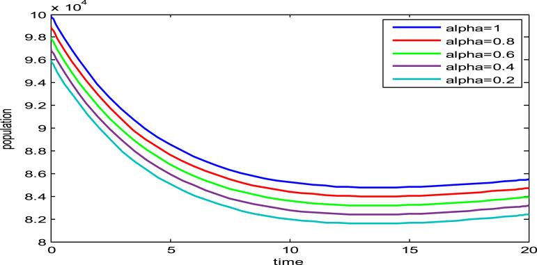
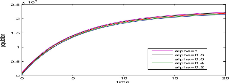
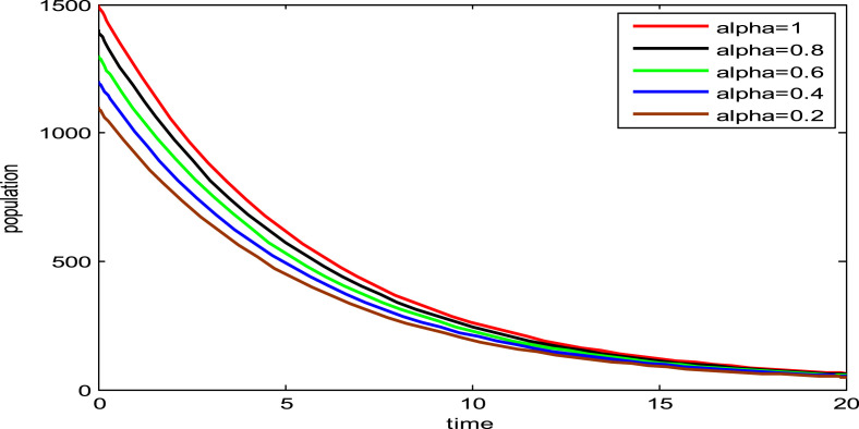
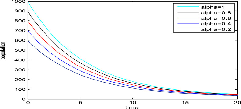
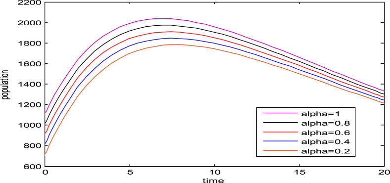
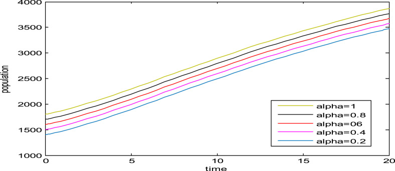
Fig. 1, Fig. 2, Fig. 3, Fig. 4, Fig. 5, Fig. 6, show the influence of the variation in the fractional order $\alpha$ on the biological behavior of the classes of model (1). It is clear from these Figures that the population of Susceptible individuals, Exposed individuals, New variant of COVID-19, Old variant of COVID-19, Hospitalized individuals and Recovered individuals have decreasing effect when $\alpha$ is decreased from $1-0.2$.

Fig. 1.

Dynamics of Susceptible individuals for various values of $\alpha$.

Fig. 2.

Dynamics of Exposed individuals for various values of $\alpha$.

Fig. 3.

Dynamics of new variant of COVID-19 for various values of $\alpha$.

Fig. 4.

Dynamics of old variant of COVID-19 for various values of $\alpha$.

Fig. 5.

Dynamics of hospitalized individuals for various values of $\alpha$.

Fig. 6.

Dynamics of Recovered individuals for various values of $\alpha$.

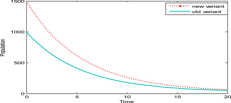
Fig. 7 compares the dynamics of new and old strain of COVID-19. This figure shows that the two variants can co-exist in the same population when their basic reproduction ratio is the same.

Fig. 7.

Dynamics of new and old variants of COVID-19..

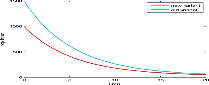
Fig. 8 shows that when $R_1>R_2$, then the new variant of COVID-19 outperform the old variant which leads to subsequent domination of the old variant by the new variant.

Fig. 8.

Dynamics of new and old variants of COVID-19 when $R_1>R_2$.

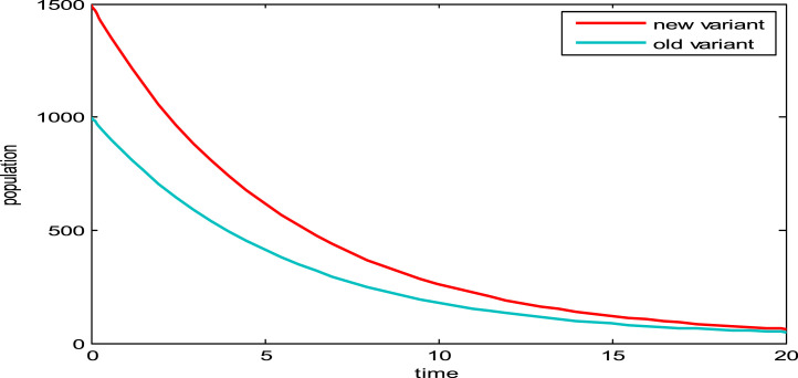
Fig. 9 shows that when $R_2>R_1$, then the old variant of COVID-19 outperform the new variant which leads to subsequent domination of the new variant by the old variant.

Fig. 9.

Dynamics of new and old variants of COVID-19 when $R_2>R_1$.

It worth mentioning here that the fractional derivative with​ $\alpha \in \left(\left(0,1\right]\right)$ is defined in Caputo–Fabrizio sense, so introducing a convolution integral with a power-law memory kernel benefits in describing memory effects in dynamical systems. The decaying rate of the memory kernel depends on $\alpha$. A lower value of $\alpha$ corresponding to more slowly-decaying time-correlation functions leads a long memory. Therefore, as $\alpha \to 1$, the influence of memory decreases.

6. Conclusion

The dynamics of COVID-19 variations were explored using a Caputo–Fabrizio fractional-order model. The model’s fundamental properties were studied. The next-generation matrix (NGM) approach was used to calculate the basic reproduction ratio ${\text{R}}_0$. Equilibrium solutions are found by equating system (1) to zero and simultaneously solving the result. Fixed point theory is used to perform a detailed study of the existence and uniqueness of the model solution. The iterative solution of the model is computed using the fractional Adams–Bashforth technique. The numerical results are shown using the estimated values of the model parameters to justify the importance of the fractional-order derivative. The graphs provide useful information about the model’s complexity and the feasibility of obtaining reliable information about it.

CRediT authorship contribution statement

Isa Abdullahi Baba: Visualization, Investigation, Supervision, Software, Validation, Writing – review & editing. Fathalla A. Rihan: Conceptualization, Methodology, Software, Data curation, Writing – original draft.

Declaration of Competing Interest

The authors declare that they have no known competing financial interests or personal relationships that could have appeared to influence the work reported in this paper.

References

- 1.Baba I.A., Hincal E. Global stability analysis of two-strain epidemic model with bilinear and non-monotone incidence rates. Eur. Phys. J. Plus. 2021;132:208. [Google Scholar]
- 2.Baba I.A., Kaymakamzade B., Hincal E. Two-strain epidemic model with two vaccinations. Chaos Solitons Fractals. 2021;106(2018):342–348. [Google Scholar]
- 3.Lin J., Andreasen V., Casagrandi R., Levin S. Traveling waves in a model of influenza A drift. J. Theoret. Biol. 2003;222:437. doi: 10.1016/s0022-5193(03)00056-0. [DOI] [PubMed] [Google Scholar]
- 4.Feng Z., Iannelli M., Milner F. A two-strain tuberculosis model with age of infection. SIAM J. Appl. Math. 2021;65:1634. [Google Scholar]
- 5.Bremermann H.J., Thieme H.R. A competitive exclusion principle for pathogen virulence. J. Math. Biol. 2021;27:179. doi: 10.1007/BF00276102. [DOI] [PubMed] [Google Scholar]
- 6.Martcheva M., Pilyugin S. The role of coinfection in multidisease dynamics. SIAM J. Appl. Math. 2021;66:843. [Google Scholar]
- 7.Nowak M., May R. Superinfection and the evolution of parasite virulence. Proc. R. Soc. Lond. Ser. B. 2021;255:81. doi: 10.1098/rspb.1994.0012. [DOI] [PubMed] [Google Scholar]
- 8.Lipsitch M., Nowak M. The evolution of virulence in sexually transmitted HIV/AIDS. J. Theoret. Biol. 2021;174:427. doi: 10.1006/jtbi.1995.0109. [DOI] [PubMed] [Google Scholar]
- 9.Martcheva M. A non-autonomous multi-strain SIS epidemic model. J. Biol. Dyn. 2021;3(2–3) doi: 10.1080/17513750802638712. 235-2. [DOI] [PubMed] [Google Scholar]
- 10.World Health Organisation . 2021. COVID-19 Weekly Epidemiological Update Edition 70. Available: https://www.who.int/docs/default-source/coronaviruse/situation-reports/20211214_weekly_epi_update_70.pdf. [Google Scholar]
- 11.Alderremy A.A., Gómez-Aguilar J.F., Aly S., Saad K.M. A fuzzy fractional model of coronavirus (COVID-19) and its study with Legendre spectral method. Results Phys. 2021 doi: 10.1016/j.rinp.2020.103773. [DOI] [PMC free article] [PubMed] [Google Scholar]
- 12.Beigi A., Yousefpour A., Yasami A., Gómez-Aguilar J.F., Bekiros S., Jahanshahi H. Application of reinforcement learning for effective vaccination strategies of coronavirus disease 2019 (COVID-19) Eur. Phys. J. Plus. 2021;136:609. doi: 10.1140/epjp/s13360-021-01620-8. [DOI] [PMC free article] [PubMed] [Google Scholar]
- 13.Ur Rahman M., Arfan M., Shah K., Gómez-Aguilar J.F. Investigating a nonlinear dynamical model of COVID-19 disease under fuzzy caputo, random and ABC fractional order derivative. Chaos Solitons Fractals. 2020 doi: 10.1016/j.chaos.2020.110232. [DOI] [PMC free article] [PubMed] [Google Scholar]
- 14.Panwar Virender Singh, Sheik Uduman P.S., Gómez-Aguilar J.F. Mathematical modeling of coronavirus disease COVID-19 dynamics using CF and ABC non-singular fractional derivatives. Chaos Solitons Fractals. 2021 doi: 10.1016/j.chaos.2021.110757. [DOI] [PMC free article] [PubMed] [Google Scholar]
- 15.Khan M.S., Samreen M., Ozair M., Hussain T., Gómez-Aguilar J.F. Bifurcation analysis of a discrete-time compartmental model for hypertensive or diabetic patients exposed to COVID-19. Eur. Phys. J. Plus. 2021;136(8):1–26. doi: 10.1140/epjp/s13360-021-01862-6. [DOI] [PMC free article] [PubMed] [Google Scholar]
- 16.Pandey P., Chu Y., Gómez-Aguilar J.F., Jahanshahi H., Aly A.A. A novel fractional mathematical model of COVID-19 epidemic considering quarantine and latent time. Results Phys. 2021 doi: 10.1016/j.rinp.2021.104286. [DOI] [PMC free article] [PubMed] [Google Scholar]
- 17.Pandey P., Gómez-Aguilar J.F., Kaabar M.K.A., Siri Z., Mousa A.A. Mathematical modeling of COVID-19 pandemic in India using Caputo–Fabrizio fractional derivative. Comput. Biol. Med. 2021 doi: 10.1016/j.compbiomed.2022.105518. [DOI] [PMC free article] [PubMed] [Google Scholar]
- 18.Martnez J.E.E., Aguilar J.F.G., Ramn C.C., Melndez A.A., Longoria P.P. Synchronized bioluminescence behavior of a set of fireflies involving fractional operators of LiouvilleCaputo type. Int. J. Biomath. 2021;11:1–24. [Google Scholar]
- 19.Martnez J.E.E., Aguilar J.F.G., Ramn C.C., Melndez A.A., Longoria P.P. A mathematical model of circadian rhythms synchronization using fractional differential equations system of coupled van der Pol oscillators. Int. J. Biomath. 2021;11 25. [Google Scholar]
- 20.Ullah S., Khan M.A., Farooq M. A fractional model for the dynamics of TB virus. Chaos Solitons Fractals. 2021;116:63–71. [Google Scholar]
- 21.Aguilar J.F.G. Fundamental solutions to electrical circuits of non-integer order via fractional derivatives with and without singular kernels. Eur. Phys. J. Plus. 2021;133:1–20. [Google Scholar]
- 22.Ndairou F., et al. Fractional model of COVID-19 applied to Galicia, Spain and Portugal. Chaos Solitons Fractals. 2021;144 doi: 10.1016/j.chaos.2021.110652. [DOI] [PMC free article] [PubMed] [Google Scholar]
- 23.Pandey P., et al. Mathematical modeling of COVID-19 pandemic in India using Caputo–Fabrizio fractional derivative. Comput. Biol. Med. 2021;145 doi: 10.1016/j.compbiomed.2022.105518. [DOI] [PMC free article] [PubMed] [Google Scholar]
- 24.Losada J., Nieto J.J. Properties of a new fractional derivative without singular kernel. Prog. Fract. Differ. Appl. 2021;1:87–92. [Google Scholar]
- 25.Muhammad A., et al. Investigation of fractal-fractional order model of COVID-19 in Pakistan under Atangana – Baleanu Caputo (ABC) derivative. Results Phys. 2021;24 doi: 10.1016/j.rinp.2021.104046. [DOI] [PMC free article] [PubMed] [Google Scholar]
- 26.Saad K.M., Aguilar J.F.G. Analysis of reaction–diffusion system via a new fractional derivative with non-singular kernel. Phys. A. 2021;509:703–716. [Google Scholar]
- 27.Abdeljawad T. Fractional operators with exponential kernels and a Lyapunov type inequality. Phys. A. 2021;313:1–12. [Google Scholar]
- 28.Abdeljawad T., Baleanu D. On fractional derivatives with exponential kernel and their discrete versions. J. Rep. Math. Phys. 2021;80:11–27. [Google Scholar]
- 29.Baba I.A., Yusuf A., Nisar K.S., Abdel-Aty A., Nofal T.A. Mathematical model to assess the imposition of lockdown during COVID-19 pandemic. Results Phys. 2021;20 doi: 10.1016/j.rinp.2020.103716. [DOI] [PMC free article] [PubMed] [Google Scholar]
- 30.Diethelm K. Springer; Berlin: 2021. The Analysis of Fractional Differential Equations: An Application-Oriented Exposition Using Differential Operators of Caputo Type. [Google Scholar]
- 31.Atangana A. Blind in a commutative world: simple illustrations with functions and chaotic attractors. Chaos Solitons Fractals. 2021;114:347–363. [Google Scholar]
- 32.Noeiaghdam S., Micula S., Nieto J.J. A novel technique to control the accuracy of a nonlinear fractional order model of covid-19: Application of the CESTAC method and the CADNA library. Mathematics. 2021;9:1321. [Google Scholar]
- 33.Caputo M., Fabrizio M. On the singular kernels for fractional derivatives. Some applications to partial differential equations. Prog. Fract. Differ. Appl. 2021;7:79–82. [Google Scholar]
- 34.Losada J., Nieto J.J. Fractional integral associated to fractional derivatives with nonsingular Kernels. Prog. Fract. Differ. Appl. 2021;7:137–143. [Google Scholar]